Comparative Study of Structural Reliability Assessment Methods for Offshore Wind Turbine Jacket Support Structures

Abstract

Offshore wind turbines (OWTs) are deployed in harsh environments often characterized by highly stochastic loads and resistance properties, thus necessitating the need for structural reliability assessment (SRA) to account for such uncertainties systematically. In this work, the SRA of an OWT jacket-type support structure is conducted, applying two stochastic methods to predict the safety level of the structure considering various design constraints. The first method refers to a commercial finite element analysis (FEA) package (DesignXplorer© from ANSYS) which employs direct simulations and the six sigma analysis function applying Latin hypercube sampling (LHS) to predict the probability of failure. The second method develops a non-intrusive formulation which maps the response of the structure through a finite number of simulations to develop a response surface, and then employs first-order reliability methods (FORM) to evaluate the reliability index and, subsequently, the probability of failure. In this analysis, five design constraints were considered: stress, fatigue, deformation, buckling, and vibration. The two methods were applied to a baseline 10-MW OWT jacket-type support structure to identify critical components. The results revealed that, for the inherent stochastic conditions, the structural components can safely withstand such conditions, as the reliability index values were found acceptable when compared with allowable values from design standards. The reliability assessment results revealed that the fatigue performance is the design-driving criterion for structural components of OWT support structures. While there was good agreement in the safety index values predicted by both methods, a limitation of the direct simulation method is in its requirement for a prohibitively large number of simulations to estimate the very low probabilities of failure in the deformation and buckling constraint cases. This limitation can be overcome through the non-intrusive formulation presented in this work.

1. Introduction

In line with the quest to battle against the energy crisis and global climate change, wind energy is found to provide a technically and economically feasible solution, making it the most promising renewable energy technology in Europe and beyond (i.e., China, United States of America (USA), etc.) [1]. Today, the vast majority of wind energy is generated from onshore wind farms. However, there is a limitation in the further growth of onshore wind farms as a result of visual impact and limited space available to deploy wind turbines. In comparison to land, there is more available space to deploy wind turbines at sea, and the wind shear is stronger at offshore locations, driving the wind industry to move offshore, currently aiming for offshore wind in Europe to reach 64.8 GW by 2030 [1,2,3,4].

With few exceptions, most of the existing offshore wind turbines (OWTs) are installed on monopile foundations in shallow waters (depths < 50 m). However, as turbines become larger (>5 MW) and as water depth increases beyond 35–50 m, monopiles become progressively uneconomical, primarily because of modal requirements that force structural dimensions to grow even beyond fabrication and installation capabilities currently available [5]. State-of-the-art research on monopile foundations can be found in References [6,7]. Space frame structures such as jackets, widely used in the petroleum industry, offer a lighter and yet stiff alternative to monopiles. Effective design of these structures from a turbine system dynamics perspective is a demanding task. Although jacket-type support structures could contribute to further developments in the offshore wind industry, research is still required to support their basic design and analysis [5,8], as well as to take into account the requirement for optimization due to both the serial production required and the nature of these unmanned structures. As a result of application-based research, several new methods and patents were developed aiming to resolve some of these issues [9,10,11,12,13,14,15,16,17,18].

In a conventional structural analysis, the environmental loads, geometric dimensions, material properties, and parameters are treated as deterministic quantities, which are often expressed in the design through characteristic values incorporating partial safety factors for consideration of uncertainties. This type of analysis is adequate in cases where randomness is relatively small. However, structures used for offshore deployment are generally complex and subjected to high uncertainties introduced by the environment, manufacturing, and operational processes. Randomness in design parameters for such systems should be systematically accounted for via stochastic modeling, allowing for a better informed and potentially optimized design that would take into consideration the life cycle of the structure and associated time-variant mechanisms of damage. Reliability analysis enables an efficient approach to better understand the response of the system to variation of an input parameter, enabling the systematic modeling of uncertainties occurring from highly complex models, loading conditions, etc. [19]. In particular, for offshore jacket foundations, soil-structure interactions and particularities of marine environments introduce considerable uncertainties (e.g., soil properties, wind, wave, and current loads, etc.), leading to the requirement of employing proper reliability analysis methods. A structural reliability model of OWT support structures requires two key components, i.e., (1) a structural model describing the structural behavior of OWT support structures, and (2) a suitable reliability assessment method which finds the reliability index $\beta$ (or the probability of failure $P_f$) of critical members with respect to the constraints [20].

Structural models for OWT support structures can be roughly classified into two groups, i.e., one-dimensional (1D) beam models and three-dimensional (3D) finite element analysis (FEA) models. In the 1D beam model, the support structure is discretized into a sequence of elastic Euler or Timoshenko beam elements. It is computationally efficient and capable of accurately modeling global structural behavior, such as deflections and modal frequencies [21]. However, it is incapable of accurately representing the structural responses at a local scale such as stress concentration effects [22]. In the 3D FEA model, the jacket foundations are usually defined by applying brick or shell elements. In comparison to the one-dimensional beam model, the three-dimensional finite element model has the capability of examining detailed stress distributions and accurately capturing structural responses within the structure. The three-dimensional finite element analysis model was extensively applied to structural modeling of wind turbine structures due to its high fidelity [1,2,23,24,25,26,27]. Thus, the 3D FEA model is adopted in this study to determine the structural responses of OWT jacket foundations.

Due to the fact that OWT jacket support structures are embedded via piles into the soil, it is important to consider soil-structure interaction in order to adequately capture their structural response. A simple method to model the soil is the p-y method, in which the soil is modeled using equivalent springs with stiffness based on soil properties. However, this method underestimates the deflection and the modal frequency. An alternative way of modeling the soil is 3D FEA with brick elements, which is capable of providing accurate and reliable results [28,29]. Considering the accuracy, 3D FEA with brick elements is adopted to model the soil later on in this study.

Several studies [30,31,32,33,34,35,36,37,38,39,40,41,42,43,44] showed that structural reliability assessment is commonly applied to assess the safety level of OWT structures. Most reliability methods are established as time-invariant; however, in numerous instances, owing to the continuous degradation of the resistance of the structure through corrosion, fatigue, etc., or due to fluctuating loads in time, reliability models should be accounted for as time-variant [45,46]. At first, the structural reliability assessment focuses on the evaluation of the reliability of each component, assuming a series system formulation where a single point failure illustrates a global failure of the structure [40,47,48]. In a second level, however, the embedded redundancy in the system is evaluated through methods such as push-over analysis, which is again based on the calculation of component reliability. Level I methods are deterministic reliability methods that only use one characteristic value to describe each uncertain variable. Common design standard formats, such as load resistance and allowable stress, belong to this category. These methods correspond to standard deterministic design methods. They can be combined with more advanced, higher-order methods in the case of partial safety factors calibration, which can optimize their application [49]. The conventional structural reliability methods include level II (approximate) reliability methods or analytical techniques which consist of the first-order reliability method (FORM) [50] and the second-order reliability method (SORM) [51], as well as level III reliability methods which include Monte Carlo Simulations (MCS). In FORM, the limit state function is approached through Taylor’s expansion, and the problem of evaluating the reliability of a complex system is translated into a problem of mathematical optimization. SORM generally performs better in cases of highly nonlinear systems than FORM, while, in other cases, the two methods give similar results. MCS involves direct simulations and, hence, reduces the uncertainty in the results due to approximations in the solution algorithm. However, its application is constrained in the calculation of high probabilities for relatively non-complex engineering systems. MCS can be incorporated with variance reduction techniques, e.g., Latin hypercube sampling (LHS), weighted Latin hypercube sampling (WLHS), importance sampling, subset simulation, etc. [19,20,45,52].

The stochastic expansion consists of intrusive and non-intrusive formulations. An intrusive formulation is one whereby the representation of uncertainty is expressed explicitly within the analysis of the system. Practically, this refers to methods that use Karhunen-Leove expansion (K-L) and polynomial chaos expansion (PCE) to directly modify the stiffness matrix of a finite element analysis procedure, such as SSFEM (spectral stochastic FEM) and stochastic Galerkin FEM. On the other hand, non-intrusive formulations, such as stochastic response surface methods [46,49], represent uncertainties in a non-explicit way and treat the analysis code as a “black box” without requiring access to the source code. Both methods employed in this research constitute non-intrusive formulations.

The first method studied in this paper accounts for the use of a commercial tool (ANSYS DesignXplorer©), which considers randomness in input variables (such as material properties, boundary conditions, loads, and geometry) and characterizes them by the joint probability density function of the input variables. Mixed moments of order higher than two are assumed to be negligible, which means that the joint probability density function can be described by the marginal distribution functions and the correlation structure. Available tools offer several statistical distribution functions to specify the marginal distribution. The probabilistic methods implemented in the DesignXplorer© include Latin hypercube sampling, all versions of the central composite design of experiment (DOE) type, Box-Behnken design DOE type, variational technology, and Monte Carlo simulations on the response surface [53,54]. More information on these probabilistic methods can be found in References [48,54]. The benefit of the tool is in its user-friendly interface and direct link with FEM modeling. However, it relies on direct simulations, which is a limitation for the order of magnitude probabilities of interest for offshore and marine applications, and which cannot be generalized and integrated with more specialized tools for more advanced analysis.

The second approach, which was developed by the authors, proposes a non-intrusive stochastic formulation, which links the structural model to a reliability analysis algorithm through approximation modeling. In this case, quadratic response surface modeling is adopted in order to map the response of the structure in the domain of stochastic variables. The benefit of this approach is that it allows for high-fidelity computational tools to be employed for the analysis in a modular way, thereby extending its applicability to various engineering problems requiring advanced modeling techniques, and further permitting coupling with analytical reliability methods such as FORM and SORM, allowing for low values of probability of failure to be calculated.

This work aims to carry out a comparison of the two methods described above for a typical OWT jacket-type support structure considering various design constraints and stochastic variables. This paper is the first of its kind to study the structural reliability of an OWT jacket-type support structure using two methods and then comparing the results, as there is no work which reported the use of the post-processing tool inbuilt in ANSYS applied to an OWT jacket-type support structure to determine the probability of failure, nor any work comparing results from the probabilistic FEA in ANSYS to a non-intrusive stochastic formulation, which is also documented in this paper. Furthermore, the proposed non-intrusive method is verified against the commercial package, allowing for further complex engineering problems to be investigated without the need for a fully integrated application-specific tool, rather than through a modular approach which can allow the use of simpler and more computational efficient tools.

2. Theoretical Background on the ANSYS DesignXplorer© Probabilistic Methods

2.1. Monte Carlo Simulation

As the name implies, Monte Carlo simulation techniques involve “sampling” at “random” to simulate artificially a large number of experiments and to observe the result. In the case of analysis for structural reliability, this means, in the simplest approach, sampling each random variable $X_i$ randomly to give a sample value ${\widehat{x}}_i$. The limit state function $G\left(x\right) = 0$ is then checked using the sample set of values ${\widehat{x}}_i$. If the limit state function is violated (i.e., $G\left({\widehat{x}}_i\right)\le 0$), the structure or structural element “fails”. The experiment is repeated many times, each time with a randomly chosen vector $\widehat{x}$ of ${\widehat{x}}_i$ values. If $N$ trials are conducted, the probability of failure is given approximately as follows [55]:

$$p_f\approx \frac{n\left(G\left({\widehat{x}}_i\right)\le 0\right)}{N},$$

(1)

where $n\left(G\left({\widehat{x}}_i\right)\le 0\right)$ is the number of trials $n$ for which $\left(G\left({\widehat{x}}_i\right)\le 0\right)$. Obviously, the number N of trials required is related to the desired accuracy for $p_f$. It is clear that, in the Monte Carlo method, a game of chance is constructed from known probabilistic properties in order to solve the problem many times over, and from that to deduce the required result (i.e., the failure probability).

2.1.1. Direct Sampling (“Crude” Monte Carlo)

The technique sketched above is the simplest Monte Carlo approach for reliability problems but not the most efficient. The basis for its application is outlined below. The probability of limit state violation may be expressed as follows [56]:

$$p_f=J={{\displaystyle \int }}^{\text{}}\dots {{\displaystyle \int }}^{\text{}}I\left[G\left(x\right)\le 0\right]f_X\left(x\right)dx,$$

(2)

where $I\left[\right]$ is an “indicator function” which is equal to one if [ ] is “true” and zero if [ ] is “false”. Thus, the indicator function identifies the integration domain. Equation (1) represents the expected value of $I\left[\right]$. If $x_j$ represents the $j$-th vector of random observations from $f_x\left(\right)$, it follows directly from sample statistics that Equation (3),

$$p_f\approx J_1=\frac{1}{N}{\displaystyle \sum }_{j=1}^{N}I\left[G\left({\widehat{x}}_j\le 0\right)\right],$$

(3)

is an unbiased estimator of $J$. Thus, Equation (3) provides a direct estimate of $p_f$. In exploiting this procedure, three matters are of interest: how to extract most information from the simulation points, how many simulation points are needed for a given accuracy, or, conversely, how to improve the sampling technique to obtain greater accuracy for the same or fewer sample points [55].

The fundamentals of the Monte Carlo simulation method are well documented in literature [48,57]. The key functionality of Monte Carlo simulation techniques is the generation of random numbers with a uniform distribution from 0–1 [54]. The DesignXplorer© uses the advanced Mersenne Twister (MT) algorithm [58]. The MT algorithm is adopted for generating uniform pseudorandom numbers. In order to accommodate Mersenne-prime period, the MT is a modified variant of a previous generator, the twisted generalized feedback shift register (TGFSR). The MT generator was implemented in portable C-code and passed stringent statistical tests, including diehard. Its merits are due to the efficient algorithms that are unique to polynomial calculations over the two-element field [58]. ANSYS also uses the inverse probability method [48] to generate random numbers with arbitrary distributions. The implementation of the inverse cumulative probability function was verified with the results published by Kececioglu [59] with matching results even for probabilities as low as ${10}^{-24}$. It uses the Latin hypercube sampling technique [60,61] to make the sampling process more efficient, as well as to ensure that the tails of the distribution of the input variables are better represented.

The interpretation of the results of a Monte Carlo simulation analysis is based on statistical methods. The statistical procedures to calculate, for example, mean values and standard deviations, and to derive histogram plots are available in textbooks on statistics and probabilistic methods (e.g., Reference [62]). For the cumulative distribution function (CDF), the data are sorted in ascending order, and the CDF of the $i$-th data point, here denoted with $F_i$, can be derived as follows [54]:

$${\displaystyle \sum }_{k=i}^N\frac{N!}{\left(N-k\right)!k!}{F}_i^k{\left(1-F_i\right)}^{N-k}=50\%.$$

(4)

In DesignXplorer©, this equation is solved numerically for $F_i$. From the CDF curve, failure probabilities, as well as the inverse probability, can be derived.

In ANSYS, sensitivities are evaluated based on correlation coefficients [62]. The stronger a result parameter is correlated with a particular input variable, the more sensitive the result parameter is with respect to the input variable.

2.1.2. Accuracy and Validity

Monte Carlo simulation methods have two major sources of inaccuracy. Of course, the number of samples cannot be infinite, but must be limited. The error due to the limitation of the number of samples can be easily quantified. As described in Reference [62], confidence intervals from statistical results of a Monte Carlo simulation can be easily obtained. In the context of finite element analysis, another source of error, which is typically overlooked, is the error due to re-meshing the geometry if geometric uncertainties are included in the probabilistic model. Furthermore, minute changes in the geometry can cause the mesh density in critical areas of the geometry to change in a non-continuous fashion. This leads to a change in the finite element results much larger than would be expected for a small geometry change. This error due to re-meshing cannot be easily quantified, but it can be minimized, if mesh controls are applied such as specifying the number of mesh divisions in critical areas of the geometry. However, this is a manual and often time-consuming operation. A method avoiding the influence of the meshing error involves variational technology.

2.1.3. Advantages and Disadvantages

The Monte Carlo simulation method does not make any simplification or assumptions in the deterministic or probabilistic model. The only assumption it does in fact make is that the limited number of samples is representative to quantify the randomness of the result parameters. The error associated with this assumption is well quantifiable as outlined above. With an increasing number of samples, the Monte Carlo simulation method converges to the true and correct probabilistic result. The Monte Carlo simulation is, therefore, widely used as the benchmark to verify the accuracy of other probabilistic methods. Another advantage is the fact that the required number of simulations is not a function of the number of input variables.

The disadvantage of the Monte Carlo simulation method is its computational cost. As a rule of thumb, addressing low probabilities of failure requires about $N_{sim}\approx \frac{100}{P_f}$ simulation loops, where $P_f$ is the targeted failure probability. Hence, if the targeted failure probability is low, then the required number of samples may be prohibitively large, making the Monte Carlo simulation method impractical for real engineering problems.

2.1.4. Variance Reduction

According to Reference [55], the variance ${\sigma }^2$ directly affects the variance of $J_1$, and the number of samples N inversely affects the variance of $J_1$. This means that the standard deviation of $\widehat{j}$ and, hence, of the Monte Carlo estimate decreases in proportion to $N^{-\frac{1}{2}}$. By comparison, for one-dimensional integration, the error in standard deviation reduces as $N^{-2}$ for the trapezoidal rule and $N^{-4}$ for Simpson’s rule [63]. Obviously, the slow convergence of the “crude” Monte Carlo method is a significant disadvantage for its practical application. One approach involves ways to reduce the variance ${\sigma }^2$ for the estimate of the probability of failure $J$. These are the so-called “variance reduction” techniques [64]. Apart from increasing the number of samples, variance reduction can be achieved only by using additional (a priori) information about the problem to be solved. The Latin hypercube sampling technique is an example of various variance reduction techniques. A good overview of the various strategies for variance reduction in general Monte Carlo work was given by References [64,65] in relation to some techniques for structural reliability calculations.

2.2. Six Sigma Analysis (SSA) Theory

2.2.1. Sample Generation

For SSA, the sample generation is based on the Latin hypercube sampling (LHS) technique by default. In the properties view for a six sigma analysis cell, sampling type can be set to either LHS or WLHS (weighted Latin hypercube sampling). LHS is a more advanced and efficient form of Monte Carlo analysis methods. With LHS, the points are randomly generated in a square grid across the design space, but no two points share input parameters of the same value. This means that no point shares a row or a column of the grid with any other point. Generally, LHS requires 20% to 40% fewer simulations loops than the direct Monte Carlo technique to deliver the same results with the same accuracy. However, that number is largely problem-dependent [53].

2.2.2. Latin Hypercube Sampling

The Latin hypercube method, originally presented in Reference [66], is a method that can represent multiple variables avoiding overlapping datasets. According to Reference [55], stratified and Latin hypercube sampling methods use the common idea that the sampling space be divided into strata (or hypercubes) and that only a few of the many possible samples may be selected in each strata (or hypercube) for inclusion in the estimation of the integral $J$. Application of the method initiates by dividing the distribution of each stochastic variable in $n$, non-overlapping intervals with equal probability. For each variable, one value should be randomly selected from each interval, and the analysis point derived from each dataset is then associated. The homogeneous allocation of intervals on the probability distribution function yields relatively small variance in the response, compared to the conventional Monte Carlo sampling. At the same time, the analysis is much less computationally demanding to generate [49].

The samples used from within each stratum (or hypercube) can be randomly selected from those that would otherwise be used; alternatively, for example, the mean or central point might be used as the one representative value. The evaluation of $J$ then uses these selected values, weighted by their probability of occurrence. Latin hypercube sampling considers all the random variables [55,64,67,68].

For convenience, consider the special case in which all the random variables $x_i \left(i = 1,\dots , n\right)$ are each divided into the same number of strata, say $N$. It is convenient also to make the divisions such that the probability of $x_i$ falling in each stratum is $1/N$. Now, select a representative value for each stratum and for each random variable. In principle, more values could be selected, but this can also be achieved by using a greater number of strata. To estimate $J$, the procedure is to use just one of the N representative values for each random variable $x_i$ (that is, selected from one of the strata) in combination with a selected representative value from each of the other random variables. This collection of representative values forms a sample set. The process is repeated, selecting from the remaining representative values, thereby forming another sample set, and so on. In the end, there will be $N$ sample sets. These can be interpreted directly as the number $N$ of sample vectors selected in Monte Carlo sampling and, thus, can be used directly in Equation (1), with evaluations of the limit state function using the present sample sets to estimate J (and, thus, $p_f$). Latin hypercube sampling can also be combined with other variance reduction techniques [68], such as importance sampling, although it is generally considered to be most suitable for small-scale simulation problems [55,56,69].

2.3. ANSYS DesignXplorer© for Structural Reliability Analysis

In order to perform the SRA, a stochastic parametric FEA model is firstly built in the ANSYS environment such that the different input parameters are assigned their corresponding distributions. Then, the developed FEA model is employed in performing a series of FEA simulations on the OWT support structure through the DoE module packaged in the DesignXplorer© facility in ANSYS, in order to map the response domain and then derive an appropriate response surface model. The purpose of the response surface is to interpolate the values in the multiple dimensions characterized by the DoE. There are several types of response surfaces as packaged in DesignXplorer© [53] which include the genetic aggregation, standard response surface full second-order polynomials, kriging algorithms, non-parametric regression, and the sparse grid. However, in this study, only the standard response surface full second-order polynomials with manual refinements is applied, along with the selection of the specification of three verification points. The response surface is interpolated from design points in the DoE. Also packaged within the response surface module is the goodness of fit metric, which is calculated for the DoE points and can be calculated for verification points to check how accurate the response surface can predict the design points. In all limit state cases, the predicted vs. observed chart should be checked to show the goodness of fit data for one or more outputs. Furthermore, the output data should be observed in order to ascertain whether most of the points fall on or near the line, which implies that the response surface predicts the values for most of the design points within its range including the verification points accurately. This indicates that the response surface is a good fit for the DoE points.

In this study, the six sigma analysis function of the DesignXplorer© module in ANSYS is used for the probabilistic assessment. Latin hypercube sampling (LHS) with number of samples equal to 1 × 10⁷ is defined and applied to all the design constraint cases. The cumulative distribution function (CDF) is used to assess the probability of failure and, hence, the reliability of the component. The cumulative distribution function value at any given point expresses the probability that the respective parameter value remains below that point. Whether this probability represents the failure probability or the reliability of the component depends on how failure is defined [53]. The corresponding reliability index $\beta$ is evaluated through appropriate statistical transformation [55].

3. Development of a Non-Intrusive, Modular Formulation for Structural Reliability Assessment

3.1. A Modular Structural Reliability Assessment Algorithm

From the same simulations executed on the ANSYS DoE tool presented in Section 2.3, the results are imported into a MATLAB code that was developed for response surface modeling, which is presented in Section 3.2 [1,2]. Figure 1 depicts the flow chart of structural reliability assessment of the non-intrusive formulation [1,2]. In brief, the analysis starts from the definition of the system, associated limit states, and determination of which variables will be considered as stochastic in the analysis. Next, a number of FEA simulations are executed by varying inputs and recording outputs related to limit states in order to map the response of the structure in the domain of stochastic variables. An appropriate method is then selected in order to approximate the response of the system and link output variables with global inputs (such as wind and wave loads). Finally, the reliability index is calculated using MCS or FORM methods. In this instance, the iterative FORM algorithm is adopted to allow for the calculation of low probabilities of failure.

3.2. Multivariate Regression

Regression analysis is a statistical process for establishing the relationship between a dependent variable and one or more independent variables. Taking the ultimate limit state (ULS) stress constraint as an example, the dependent variable (i.e., maximum von Mises stress, ${\sigma }_{VM,max}$) and independent variables (i.e., thrust load $x_1$, tilting moment $x_2$, torsional moment $x_3$, total hydrodynamic load (wave and current) $x_4$, soil 1 Young’s modulus $x_5$, soil 2 Young’s modulus $x_6$, soil 3 Young’s modulus $x_7$, and weight of rotor-nacelle assembly (RNA) $x_8$) are assumed to have the following functional relationship:

$${\sigma }_{VM,max}=\left[a_0,a_1, \dots ,a_{16}\right]\left[\begin{array}{c}1\\ x_1\\ x_1^2\\ .\\ .\\ .\\ x_8\\ x_8^2\end{array}\right],$$

(5)

where ($a_0,a_1, \dots ,a_{16}$) are 17 regression coefficients for a quadratic regression. For other types of constraints, i.e., deformation, buckling, vibration, and fatigue, expressions similar to Equation (5) can be derived. Multivariate regression can be used to obtain the regression coefficients for different limit states [49].

Taking the stress constraint case as an example, 300 stochastic FEA simulations were performed, obtaining 300 samples. The R-square value obtained in the regression analysis performed in this case was consistently higher than 0.95, which is relatively high and indicates a satisfactory multivariate regression to be used in this study.

3.3. FORM (First-Order Reliability Method)

Having obtained the performance function from regression, FORM is used to calculate the reliability index $\beta$. The FORM Hasofer and Lind algorithm is summarized below [70].

• Define the performance function for different limit states. For example, in the ULS (stress constraint) case, Equation (5) is substituted into Equation (21), which yields the following performance function:

  $$g_u\left(x\right)={\sigma }_{VM,allow}-\left[a_0,a_1, \dots ,a_{16}\right]\left[\begin{array}{c}1\\ x_1\\ x_1^2\\ .\\ .\\ .\\ x_8\\ x_8^2\end{array}\right].$$

  (6)
• Set the mean value point as an initial design point, i.e., $x_{i,k}={\mu }_{x_i}$ $i=1,2,\dots ,n$, and calculate the gradients $\nabla g\left(X_k\right)$ of the limit-state function at this design point. Here, $x_{i,k}$ refers to the $i$-th element in the vector $X_k$ of the $k$-th iteration, and ${\mu }_{x_i}$ is the mean value of the $i$-th element.
• Calculate the initial reliability index $\beta$ using the mean-value method, i.e., $\beta =\frac{{\mu }_{\tilde{g}}}{{\sigma }_{\tilde{g}}}$ and its direction cosine $\alpha$.

  $$\beta =\frac{{\mu }_{\tilde{g}}}{{\sigma }_{\tilde{g}}}=\frac{g\left({\mu }_X\right)}{{\left[{{\displaystyle \sum }}_{i=1}^n{\left(\frac{\partial g\left({\mu }_X\right)}{\partial x_i}\right)}^2.{\sigma }_{xi}^2\right]}^{\frac{1}{2}}}.$$

  (7)

  $${\alpha }_i=-\frac{\left(\frac{\partial g\left(X^{\ast }\right)}{\partial x_i}\right).{\sigma }_{x_i}}{\sqrt{{{\displaystyle \sum }}_{i=1}^n{\left(\frac{\partial g\left(X^{\ast }\right)}{\partial x_i}{\sigma }_{x_i}\right)}^2}}.$$

  (8)
• Compute a new design point $X_k$ and $U_k$, function value, and gradients at this new design point.

  $$x_{i,k}={\mu }_{x_i}+\beta {\sigma }_{x_i}{\alpha }_i.$$

  (9)

  $$u_{i,k}=\frac{x_{i,k}-{\mu }_{x_i}}{{\sigma }_{x_i}}.$$

  (10)
• Compute the reliability index $\beta$ and direction cosine ${\alpha }_i$ using Equations (9) and (10), respectively.

  $$\beta =\frac{g\left(U^{\ast }\right)-{{\displaystyle \sum }}_{i=1}^n\frac{\partial g\left(U\right)}{\partial x_i}{\sigma }_{x_i}{u}_i^{\ast }}{\sqrt{{{\displaystyle \sum }}_{i=1}^n{\left(\frac{\partial g\left(U^{\ast }\right)}{\partial x_i}{\sigma }_{x_i}\right)}^2}}.$$

  (11)

  $${\alpha }_i=-\frac{\left(\frac{\partial g\left(X^{\ast }\right)}{\partial x_i}\right).{\sigma }_{x_i}}{\sqrt{{{\displaystyle \sum }}_{i=1}^n{\left(\frac{\partial g\left(X^{\ast }\right)}{\partial x_i}{\sigma }_{x_i}\right)}^2}}.$$

  (12)

Repeat steps 4–5 until the convergence of the reliability index $\beta$ is achieved.

4. Design Load Analysis

4.1. Sources of Loads

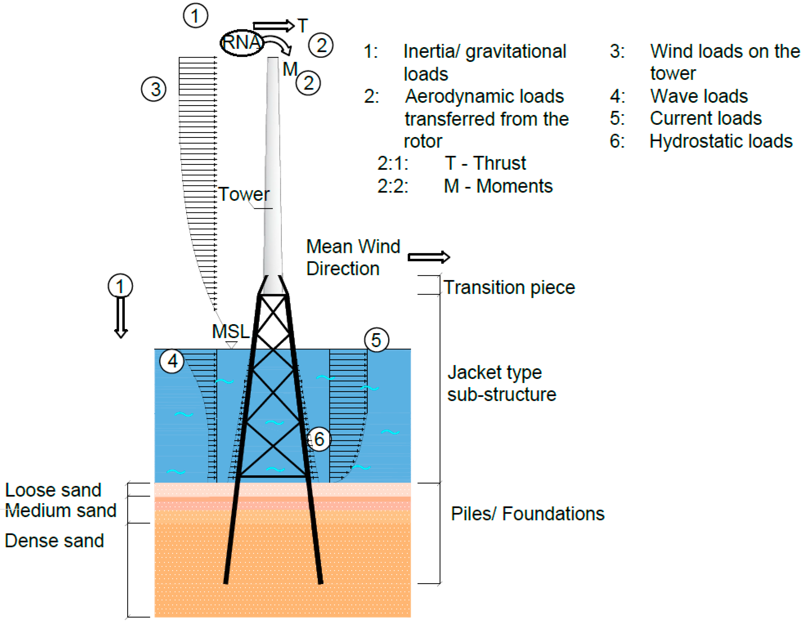
OWTs are exposed to several load sources usually imposed by their environment. In design codes, such as DNV-OS-J101 [71] and IEC 61400-3 [72], loads which are relevant to the design of OWT jacket support structures are outlined. Calculations and formulations of each load produced by the environment in this study are based on DNV-RP-C205 [73]. The loads relevant to OWT support structures can be roughly classified into six groups, i.e., (1) aerodynamic loads transferred from the rotor, (2) wind loads on the tower, (3) inertia loads, (4) current loads, (5) wave loads, and (6) hydrostatic loads [24]. These loads are illustrated in Figure 2.

Gravitational and inertia loads are static and dynamic loads which result from seismic activity, the entire structure’s weight and imposed equipment on the structure under operation, and the exerted forces on the structure due to operations [74]. The inertia loads, as a result of the support structure and rotor-nacelle assembly (RNA) weight at the tower top, can have a significant impact on buckling and considerably influence the eigen-frequencies of the OWT support structure [24].

Aerodynamic loads are dynamic and static loads resulting from the airflow interaction with the moving and stationary wind turbine components. The load magnitude varies, and this depends on the air density, the mean wind speed and turbulence across the rotor plane, and the aerodynamic shapes of the components of the wind turbine and their interactive effects. These loads can be computed using aeroelastic models [74]. The aerodynamic loads imposed by the rotor are transmitted to the top of the tower and are usually decomposed into a load matrix defined in the referential axis of the wind turbine. The fatigue loads were determined by employing the damage equivalent load (DEL) method, which was described in Reference [75]. The support structure was subjected to thrust load directed along the diagonal of the jacket base and applied at the assumed RNA center of mass (CM). This loading set-up resembled a yaw error situation and produced an additional torsional moment at the tower top. The presence of a horizontal offset for the RNA CM led to a gravity moment at the tower top [8]. Wave load and rotor thrust vectors were directed along the jacket base diagonal, causing maximum compression and tension on the opposite legs [5].

Environmental loads are those caused by environmental phenomena, i.e., the set produced by wave force, current force, and wind force. Wave loads are dynamic loads produced by waves and their interaction with the OWT support structure. Le Mehaute’s graph indicates the validity range of each wave theory and can be employed to determine the most applicable theory for given characteristics of waves, such as wave period (T), wave height (H), and water depth (d) [74]. The regular wave theories are ideal for designs where a single wave method is adopted, and this is a widely used method in offshore structure design. In this case, a regular wave with the appropriate period and height is used to represent an extreme wave. This method provides an easy analysis in estimating the extreme response of offshore structures. On the other hand, the random ocean wave is defined by an energy density spectrum. The ocean wave energy content and its distribution over a random wave frequency range are described by the wave energy spectrum. Therefore, the random wave design method may be ideal for designing floating structures [76]. In this study, the wave profile data presented in

Table 1. Water levels and wave data of interest for the K-13 deep-water site.

Parameter	Value
Lowest astronomical tide, LAT (m)	−1.06
Tidal range, $\Delta z_{tide}$ (m)	2.22
Storm surge, $\Delta z_{surge}$ (m)	2.13
Air gap, $\Delta z_{air}$ (m)	1.5
Significant wave height, $H_s$ (m)	9.4
Maximum 50-year wave height, $H_{50,max}$ (m)	17.48
Maximum wave period range, $T_{50}$ (s)	10.8–14
Maximum wave height above still water for deck height calculation, ${\xi }_w$ (m)	11.36

fall within the area of validity of the Stokes third-order wave theory. Stokes wave theory is one of the most commonly used methods in the analysis of offshore structures because of its accuracy in predicting the kinematic properties of the wave.

A typical bottom-fixed jacket offshore structure is considered to be dominated by drag owing to the wavelength, water depth, structural shape, and size; thus, Morison’s equation is adopted. An assumption that the total force due to waves acting on a structure can be computed by the linear superimposition of the drag and inertia forces is made in Morison’s equation. For Morison’s equation to be applied to determine the wave loads acting on the structure, the member diameter, $D$, has to be less than one-fifth of the wavelength, $\lambda$, i.e.,

$$D\le 0.2\lambda .$$

(13)

For slender members such as jacket members submerged in water, both current and wave loads can be determined using Morison’s equation [71].

$$F=F_d+F_m=\frac{1}{2}{\rho }_w{C}_{d}D\left|u_x\right|u_x+{\rho }_w{C}_m\frac{\pi D^2}{4}{a}_x,$$

(14)

where the drag force is the first term while the inertia force is the second term; ${\rho }_w$ is the density of water; $C_d$ and $C_m$ are the drag and inertia coefficients of the pile, respectively, and their corresponding values are 1.25 and 2.0, respectively [5]; $D$ is the cylinder diameter; $a_x$ and $u_x$ are the horizontal wave-induced or current-induced acceleration and velocity of water, respectively, which were derived from the Stokes third-order theory.

Current loads are dynamic loads which are produced by the flow of water from external sources, apart from surface waves. Current can cause drag loads on the support structure. The current velocity $u_c\left(z\right)$ is described by a sub-surface current exponential profile from the mean sea level (MSL) to the seabed, $d$. The total current velocity of a submerged, stationary, tubular member, in the absence of vortex shedding, can be calculated as follows:

$$u_c\left(z\right)=u_{c,MSL}{\left(\frac{d+z}{d}\right)}^{1/7},$$

(15)

where $u_{c,MSL}$ is the current velocity at MSL, and $d$ is the depth of water from MSL to the seabed. The wave particle velocity and the current velocity are summed up in Morison’s drag term in Equation (14), assuming that the wave and current are aligned.

The wind loads on the tower structure are a result of the drag and a function of the average wind velocity $\overline{V}\left(z\right)$. The wind shear is generally represented by a power law profile, defined by the following equation:

$$\overline{V}\left(z\right)={\overline{V}}_r{\left(\frac{Z}{Z_r}\right)}^{\alpha },$$

(16)

where ${\overline{V}}_r$ denotes the reference wind speed at the elevation of nacelle altitude $Z_r$, and α is the roughness coefficient with a value of 0.115 for the offshore site [24]. Wind loads acting along the tower can be calculated as follows:

$$F_{tower}\left(z\right)=\frac{1}{2}{\rho }_a{C}_{D,T}D\left(z\right){\overline{V}}_r^2\left(z\right),$$

(17)

where $C_{D,T}$ is the coefficient of drag of the tower, with a typical value of 1.0 [24], and $D\left(z\right)$ represents the external diameter of tapered tower at height $z$. Having determined the wind loads, the moments due to the action of the wind loads can then be calculated.

Hydrostatic pressure, which acts on the submerged sections of the jacket support structure, is a constant normal load and varies with the depth of water. The hydrostatic force can be expressed as

$$F_h={\rho }_{w}gh,$$

(18)

where $F_h$ is the hydrostatic force, $g$ is the acceleration due to gravity, and $h$ is the depth of the water.

4.2. Site Specifications and Design Load Cases

The design load cases should take into account a set of design situations considering the most critical conditions that an OWT support structure can be subjected to, combining extreme or standard external conditions with operational states of the wind turbine or other operational modes (such as installation, transportation, fault, or maintenance) [74]. For the structural design of OWTs, IEC61400-3 [72] outlines 32 DLCs (design load cases) consisting of all operational modes of an OWT, which include start-up, standard operation, shut down, and 50-year extreme conditions. These DLCs can be roughly categorized into two main groups, namely, ultimate and fatigue. Basically, the typical load cases adopted in the structural design of OWTs are mainly the fatigue load considering normal sea conditions and the ultimate load considering 50-year extreme conditions. Both the fatigue and the ultimate load cases are considered in this study.

4.2.1. Fatigue Load Case

Due to the nature of rotor operation, as well as hydrodynamic loading, a significant source of periodic loadings is imposed during the lifetime of an OWT. OWT support structures are, thus, prone to fatigue failure [24,77]. A widely used fatigue DLC correlates to an operating state within the normal sea state (NSS) and normal turbulence model (NTM), where the site is assumed to have no current and both the wave height and the cross zero period are obtained via a probability density function of the site. DLC 1.2, as prescribed in the IEC standard [72], are generally regarded as the governing fatigue DLCs for OWT support structures; therefore, they are considered in this study as fatigue load cases [24,78]. According to the IEC standard [79,80], the safety factor for fatigue load is equivalent to 1.0.

4.2.2. Ultimate Load Case

For the extreme hydrodynamic loads experienced by the OWT, that produced by the 50-year return period is widely considered as a critical ultimate load case. It was demonstrated from a previous study that wind loading generally governs the design of OWTs rather than hydrodynamic loading [81]. Therefore, the critical load case for ULS is mostly assumed to be defined by the parked turbine, under the 50-year EWM (extreme wind model) with 50-year RWH (reduced wave height) and ECM (extreme current model). The loading characteristics, as described above, correspond to the IEC 61400-3 [72] DLC 6.1b and 2.1 GL regulation [82], respectively. Load safety factors for gravitational and other loads (such as environmental loads) are given as 1.1 and 1.35, respectively [79,80].

4.2.3. Site Specifications

The information available from a previous study for a deep-water site located off the coast of Netherlands designated as the K-13 deep-water site [80] was adopted for this study, as listed in Table 1.

5. Baseline 10 MW OWT

There is continued interest in increasing the size of offshore turbines given the high cost of the support structure and associated operation and maintenance (O&M) activities. The baseline 10-MW OWT [5,8,83] is an envisioned simple reference 10-MW turbine scaled from a 5-MW NREL (national renewable energy laboratory) reference turbine [84]. The main properties were calculated through basic mechanics considerations and scaling laws. The RNA (rotor-nacelle assembly) is supported by an 88.4-m tapered tubular tower. Its basic characteristics are summarized in

Table 2. Main properties of the baseline 10-MW OWT model [5].

Item	Value
Rated power (MW)	10
Blade length (m)	87.70
Hub radius (m)	3.05
Rotor diameter (m)	181
Tip radius (m)	90.74
Rotor-nacelle assembly mass (kg)	1,072,000
Blade vertical clearance (m)	2
Precone (°)	3
Shaft tilt (°)	−5
Overhang (m)	−9.10

, and further details can be found in References [5,8].

5.1. Parametric FEA

A parametric finite element analysis model of the OWT support structure and the soil system was developed using ANSYS software package, a widely used multi-purpose finite element analysis software. The parametric FEA model enables modeling OWT support structures with stochastic variables, such as environmental loads and material properties. The environmental loads, i.e., wind, wave, and current loads, are applied to the structure in an uncoupled way, ignoring the fluid-structure interactions, as illustrated in Figure 2. The parametric FEA model is applied to the jacket support structure of the baseline 10-MW OWT, of which the main parameters are summarized in

Table 3. Baseline 10-MW support structure parameters [5,8,80,83]. MSL—mean sea level; OD—outer diameter; TP—transition piece; RNA—rotor–nacelle assembly; UL—ultimate limit; FL—fatigue limit.

Parameter	Value
Deck height above MSL (m)	16
Water depth (m)	50
Leg OD (m)	1.74
Leg wall thickness (m)	0.030
Number of bays	4
Jacket batter	8.47
Height of TP (m)	7
Number of legs	4
Pile OD (m)	1.59
Pile wall thickness (m)	0.037
Mud brace OD (m)	0.762
Mud brace wall thickness (m)	0.017
x-brace outer diameter (m)	0.61
x-brace wall thickness (m)	0.016
RNA mass (kg)	1,072,000
Tower length (m)	88.4
Tower-top OD (m)	3.85
Tower-top thickness (m)	0.03
Tower-base OD (m)	7
Tower-base thickness (m)	0.055
Thrust associated with rated power UL case (kN)	1700
Maximum rotor thrust taking into account dynamic amplification UL case (kN)	3400
Thrust FL case (kN)	203
Torsional moment UL case (kN∙m)	7876
Torsional moment FL case (kN∙m)	3483
Tilting moment UL case (kN∙m)	38,567
Tilting moment FL case (kN∙m)	3687

. The geometry, material, mesh, and boundary conditions used in the FEA model are presented in the upcoming subsections.

5.1.1. Geometry

The configuration of the jacket is usually a structure with four legs, inter-connected with bracings welded with diameters up to 2 m. A transition piece is connected to the tower bottom and transfers the forces from the tower into the jacket structure, which is anchored via piles or suction caissons to the seabed at each leg. The jacket structure has a vertical height of 66 m, and it is joined with the tower through a 7-m-long transition piece. The transition piece is envisioned as a deck reinforced by stringers, which hosts a central cylindrical shell supported by four tubular struts. The piles are embedded 42 m in the soil and are intended to be driven through the legs and, thus, feature a batter angle [5,8].

5.1.2. Mesh

A crucial step in the coupling of the model to be applied for the FEA is the mesh generation. The ANSYS software package provides a powerful and reliable structure mesh generator capable of developing a mesh, which is consistent in all of the structure with minimal computational requirement.

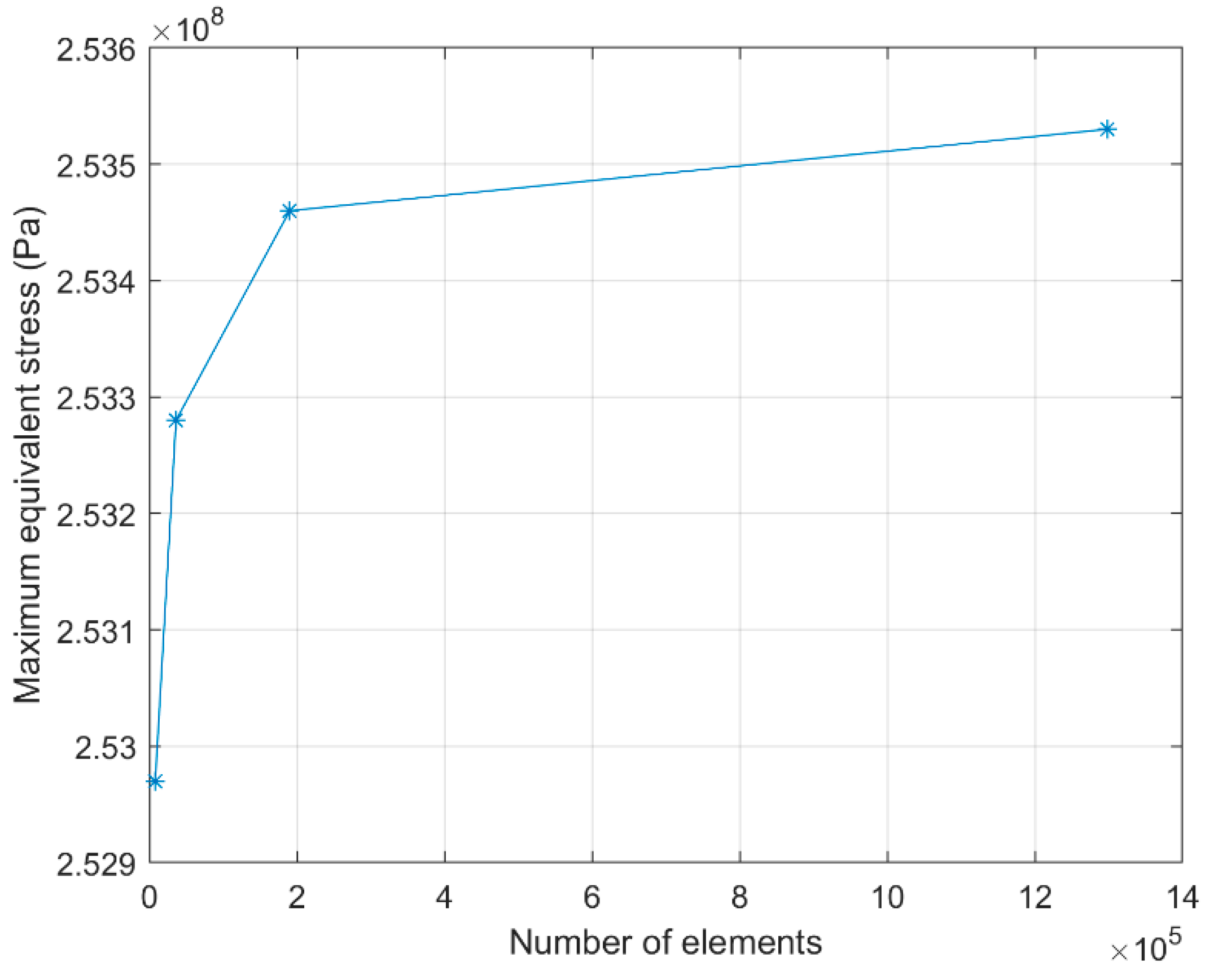
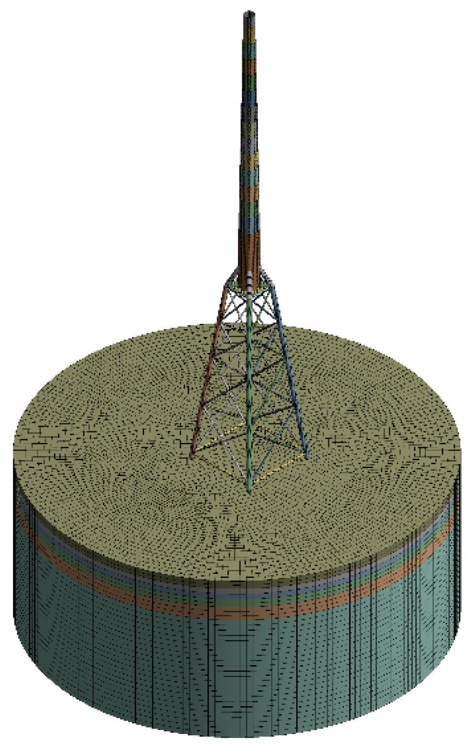
In order to ensure accuracy of results, a mesh sensitivity study was carried out [1,24]. This is depicted in

Table 4. Mesh sensitivity.

Soil Element Size (m)	Jacket Structure Element Size (m)	Number of Elements	Maximum von Mises Stress (Pa)	Maximum Displacement (m)	Buckling Load Multiplier
8	2	8047	$2.5297\times {10}^8$	1.2492	3.7286
4	1	36,164	$2.5328\times {10}^8$	1.2492	3.7286
2	0.5	190,222	$2.5346\times {10}^8$	1.2492	3.7286
1	0.25	1,298,092	$2.5353\times {10}^8$	1.2492	3.7286

and Figure 3. From the mesh sensitivity study, the equivalent (von Mises) stress converged at the mesh size of 2 m for the soil and 0.5 m for the support structure, corresponding to a total number of elements of 190,222. Therefore, 2 m and 0.5 m are deemed as appropriate mesh sizes for the soil and the support structure, respectively. As can be observed, the maximum displacement and buckling load multiplier are not sensitive to change in mesh size. The generated mesh for the FEA model is depicted in Figure 4.

5.1.3. Material

The jacket structure is made of S355 structural steel with a density of 8500 kg/m³ (increased by 8% to cover for secondary steel appurtenances, coatings, and welds that are not covered for in the thickness data of the support structure), Young modulus of 210 GPa, a Poisson’s ratio of 0.3, and a nominal yield strength of 355 MPa. The tower and the transition piece are made of structural steel of the same properties [5,24].

5.1.4. Soil Profile

Other than the OWT support structure, a crucial section of the detailed parametric model comprises the soil-structure interaction, which is a factor of design of significant importance for the structural response of the piles-jacket-tower assembly. The soil modeled in the FEA model is cylindrical in shape, with a diameter of 140 m and height of 50 m and consisting of six different strata (see

Table 5. K-13 deep-water site’s soil profile [5].

Depth below Seabed (m)	Unit Weight N/m3	Friction Angle (°)	Shear Strength (N/m2)	Young’s Modulus (MPa)
0–3	10,000	36	60,000	30
3–5	10,000	33	60,000	30
5–7	10,000	26	60,000	50
7–10	10,000	37	60,000	50
10–15	10,000	35	60,000	50
15–50	10,000	37.5	60,000	80

). The soil material is modeled using the Drucker-Prager strength linear model [85]. This model is used to calculate the yield strength of each soil strata. The yield strength of the soil, ${\sigma }_{ys}$, according to the Drucker-Prager model, is given by

$${\sigma }_{y,s}=\frac{6c\cos \varphi }{\sqrt{3}\left(3-\sin \varphi \right)},$$

(19)

where $\varphi$ represents the internal friction angle, and $c$ represents the cohesion value. The coefficient of friction $C_f$ between the soil and the pile is determined as follows [28]:

$$C_f=\tan \left(\frac{2}{3}\varphi \right).$$

(20)

5.1.5. Boundary Conditions

The wind and wave loads are applied to the surface of the tower and the surface of support structure submerged into the water, respectively. Additionally, the following three boundary conditions are also defined: (1) the bottom of the soil model is fixed against translation in all directions; (2) lateral boundaries of the soil model are fixed against lateral translation; (3) an augmented Lagrangian formulation-based frictional contact [86,87] is established between the soil and pile with suitable friction coefficients in order to enable soil-structure interaction. See Figure 5.

5.2. Validation of the FEA

5.2.1. Modal Analysis

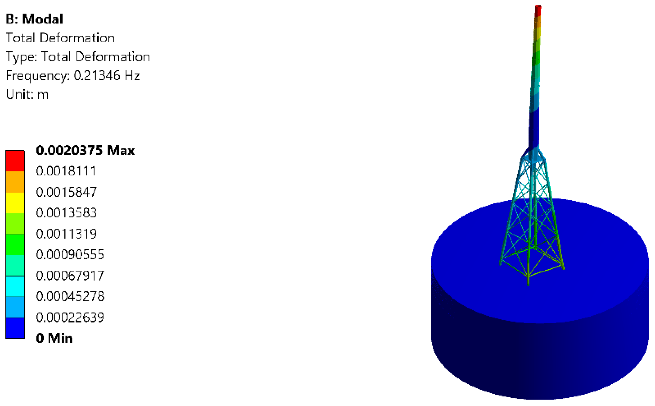
The modal frequencies of the OWT support structure calculated from the present FEA model are compared against those reported in the literature. The comparison results are presented in

Table 6. Comparison of the support structure mode frequencies with reference values.

Mode Frequencies (Hz)	Present	References [8,83]	% Difference
1st side-to-side bending	0.21346	0.21320	0.12%
1st fore-aft bending	0.22297	0.21629	2.99%
2nd side-side bending	1.1602	1.0313	11.11%
2nd fore-aft bending	1.5292	1.6561	−8.29%

. As can be observed in Table 6, the first two frequencies of both fore-aft and side-to-side bending modes calculated from the present FEA model show good agreement with those reported in References [8,83], with the maximum percentage difference (11.11%) observed for the second side-to-side bending mode. This confirms the validity of the present FEA model. See Figure 6.

5.2.2. Deflections in Static Analysis

This section of the validation aims to examine the deformation behavior of the support structure in a static analysis. In the literature [5,8], the RNA weight and a 3.4-MN thrust load were applied on the tower top. The displacements at the RNA elevation and the base of the tower are compared with reference values, and results are presented in

Table 7. Static deformation of the baseline 10 MW on jacket.

Load Case	Displacement at RNA			Displacement at the Tower Base
Mass/thrust	Present	Reference [8]	% Difference	Present	Reference [8]	% Difference
RNA/3.4 MN	1.263 m	1.2688 m	−0.46%	$1.6085\times {10}^{-1}$	$1.6639\times {10}^{-1}$	−3.44%

. Under the loaded condition, the deflections at the RNA and at the tower base are measured with respect to the location of the RNA and the center of the tower base, respectively.

As can be observed from Table 7, the results of the present FEA model match well with those reported in Reference [8], for deflections at both the RNA and the tower base, with a maximum difference of 3.44% observed for the deflection at the tower base. This further confirms the validity of the present FEA model. See Figure 7.

6. Implementation of Structural Reliability Assessment on the OWT Support Structure

In this section, the structural reliability of the OWT support structure is assessed considering three limit states according to DNV-OS-J101, i.e., (1) ultimate limit state (ULS), (2) fatigue limit state (FLS), and (3) serviceability limit state (SLS). The fully parametric FEA model presented in Section 5.1 is used to perform FEA modeling taking account of stochastic variables. The results are then post-processed using two methods, i.e., (i) using the probabilistic FEA tool packaged in ANSYS referred to as the DesignXplorer©, and (ii) applying the non-intrusive formulation as described in Section 2 and References [2,49].

6.1. Constraints and Design Criteria

In the design of OWT support structures, three limit states should be considered according to DNV-OS-J101, i.e., (1) ULS (ultimate limit state), which accounts for the maximum load-carrying capacity (i.e., buckling and yielding stress), (2) FLS (fatigue limit state), which accounts for failure as a result of cyclic loads, and (3) SLS (serviceability limit state), which accounts for tolerance criteria (i.e., vibrations and deflections) applicable to standard use. Thus, the structural reliability of OWT support structures in this study takes into consideration five design criteria, i.e., stress (ULS), vibration (SLS), buckling (ULS), deformation (SLS), and fatigue (FLS).

6.1.1. Stress Constraint

The ULS (ultimate limit state) defines the ability of the structure to resist yielding. In terms of ultimate limit state, the maximum stress in the support structure ${\sigma }_{VM, max}$ should not exceed the allowable stress limits ${\sigma }_{VM, allow}$. The limit state function for the von Mises criterion can be expressed as follows:

$$g_u\left(x\right)={\sigma }_{VM,allow}-{\sigma }_{VM,max}.$$

(21)

The allowable stress ${\sigma }_{VM, allow}$ can be expressed as follows:

$${\sigma }_{VM, allow}=\frac{{\sigma }_y}{{\gamma }_m},$$

(22)

where ${\sigma }_y$ is the yield strength, with a value of 355 MPa for steel S355, and ${\gamma }_m$ is the material safety factor, with a value of 1.1 suggested by DNV-OS-J101 standard [71]. Thus, the allowable stress ${\sigma }_{VM, allow}$ is 323 MPa.

6.1.2. Fatigue Constraint

The fatigue limit state is a crucial phenomenon in OWT support structures as they are subjected to significant cyclic loads. OWT support structures normally have a long service period that may exceed 20 years. This, in conjunction with the inspection intervals, affects the reliability requirement of the jacket structural design. According to the S-N curve method, the number of loading cycles to failure $N$, can be obtained by

$$logN=A-mlog\Delta S,$$

(23)

where $A$ and $m$ are the intercept and the slope of the S-N curve on the log-log plot, respectively; $\Delta S$ is the stress range. The two parameters in Equation (23), i.e., intercept $A$ and slope $m$, are generally given by design standards, e.g., DNVGL-ST-0126 [29]. The performance function of fatigue reliability assessment based on the S-N curve method can be expressed as follows:

$$g_{f, SN}=logN-log{N}_t,$$

(24)

where subscripts $f$ and $SN$ denote the fatigue limit state and S-N curve method, respectively; $N$ is the number of loading cycles to failure given by Equation (23), and $N_t$ is the number of loading cycles expected during the given design life. The number of cycles during the design life $N_t$ may be determined as a function of rated rotor speed $n_{rated}$ and availability ${\eta }_a$ (98.5%) on the location chosen [24,88]. Therefore, considering a design life of 20 years, the number of cycles can be expressed as follows:

$$N_t={\eta }_a.n_{rated}\times \left(20\left[year\right]\times 365\left[day/year\right]\times 24\left[hour/day\right]\times 60\left[min/hour\right]\right).$$

(25)

The minimum fatigue safety ratio $f_{sr, min}$ must be greater than the allowable fatigue safety ratio $f_{sr,allow}$, which is equivalent to the product of one and the material PSF (partial safety factor) ${\gamma }_{m,f}$ for fatigue.

$$f_{sr,min}\ge f_{sr,allow}.$$

(26)

Since the material’s PSF for fatigue limit state is 1.15 [29], $f_{sr,allow}$ is equivalent to 1.15. Hence, the limit state function based on the fatigue safety ratio can be expressed as follows:

$$g_{f,f_{sr} }=f_{sr,allow}-f_{sr,min}.$$

(27)

6.1.3. Deformation Constraint

Excessive deflections influence the serviceability of OWT support structures and, therefore, should be avoided. The allowable deflection $d_{allow}$ must exceed the maximum deflection $d_{max}$ to ensure overall structural stability. This can be expressed as

$$d_{allow}>d_{max}.$$

(28)

The limit state function for deflection criteria can be expressed as

$$g_d\left(x\right)=d_{allow}-d_{max}.$$

(29)

The allowable deflection $d_{allow}$ is given by the following empirical equation as suggested by DNV-OS-J101 [71]:

$$d_{allow}=\frac{L}{200},$$

(30)

where $L$ is the height of the jacket.

6.1.4. Buckling Constraint

The slenderness of the support structure coupled with the large RNA mass at the tower top forces the investigation of the risk of instability as a result of buckling. The ULS static analysis results are employed as pre-stress loads. The load multiplier $L_m$, which is defined as the critical load divided by the present load applied, should exceed the permissible load multiplier, $L_{m,allow}$ in order to avoid failure. This design criterion is given as

$$L_m\ge L_{m,allow}.$$

(31)

According to the DNV standard [29], 1.4 is adopted as the $L_{m,allow}$ value in this study. The limit state function for buckling criteria can, thus, be expressed as

$$g_b\left(x\right)=L_m-L_{m,allow}.$$

(32)

6.1.5. Vibration Constraint

One of the critical concerns for OWTs on jacket support structures is the resonance phenomenon. In order to guard against such a phenomenon, the first eigen-frequency $f_{1st}$ of the OWT support structure must be separated sufficiently from rotor induced frequencies $f_{1P}$ and blade-passing frequency $f_{3P}$. A soft-stiff structural design, whereby the modal frequency lies between the rotor upper bound $f_{1P}$ ($f_{1PH}$) and lower bound $f_{3P}$ ($f_{3PL}$) frequencies, is presently the most usual and cost-effective design for a jacket. Therefore, the resonance constraint should be expressed as follows [5,24,89]:

$$f_{1PH}\le f_{1st}\le f_{3PL},$$

(33)

$$0.133\le f_{1st}\le 0.233.$$

(34)

The limit state function for the resonance criterion at the rotor upper bound can, thus, be expressed as

$$g_r\left(x\right)=f_{1st}-f_{1PH}.$$

(35)

On the other hand, it is expressed at the rotor upper bound as follows:

$$g_r\left(x\right)=f_{3PL}-f_{1st}.$$

(36)

The lower g-function value is chosen to be applied in the reliability assessment.

6.2. Stochastic Variables and FEA

The stochastic variables considered in this study are presented in

Table 8. Stochastic variables.

Description	Distribution Types
Wind thrust	Normal [2,90,91]
Tilting moment	Normal [2]
Torsional moment	Normal [2]
Weight of RNA	Normal [90,91]
Young’s modulus of soils	Normal [2,90,91]

. Eight stochastic variables were considered for all cases (i.e., wind thrust, tilting moment, torsional moment, the weight of RNA, hydrodynamic load, and three Young’s moduli were considered at three soil strata). The total hydrodynamic load is considered differently, based on its dependence on the wave height, wave period, and current speed. To find the peak hydrodynamic force acting on the system, a Weibull distribution is applied to the significant wave height and the current speed, while the lognormal distribution is applied to the wave period [2,90,91]. The distribution is then fitted into a Weibull-equivalent distribution. In the presence of observed data, distribution fitting algorithms (such as Akaike information criterion, Bayesian information criterion, and Kolmogorov-Smirnov) are often employed to determine the shape coefficients of the most appropriate statistical distributions [19]. The coefficient of variation (COV) of all stochastic variables was assumed to be 0.1 except for the stochastic variables with Weibull distribution. The mean values of these stochastic variables are presented in Table 2, Table 4, and Table 5. This is summarized in

Table 9. Characteristics of design variables.

Description	Ultimate Load Case		Fatigue Load Case
	Mean	Standard Deviation	Mean	Standard Deviation
Wind thrust (kN)	1700	170	203	20.3
Tilting moment (kN∙m)	38,567	3856.7	3687	368.7
Torsional moment (kN∙m)	7876	787.6	3483	348.3
RNA mass (kg)	1,072,000	107,200	1,072,000	107,200
Young’s modulus of soil stratum 1 (MPa)	30	3	30	3
Young’s modulus of soil stratum 2 (MPa)	50	5	50	5
Young’s modulus of soil stratum 3 (MPa)	80	8	80	8

, which depicts the means and the corresponding standard deviations. Having defined the stochastic variables, the FEA model presented in Section 5.1 is then used to perform FEA simulations of the OWT support structure with the help of the design of experiments (DoE) module in ANSYS. It enables the input parameters to be designated as stochastic parameters, having different types of distributions. DoE indicates the variation of design points with the output parameter.

7. Results and Discussion

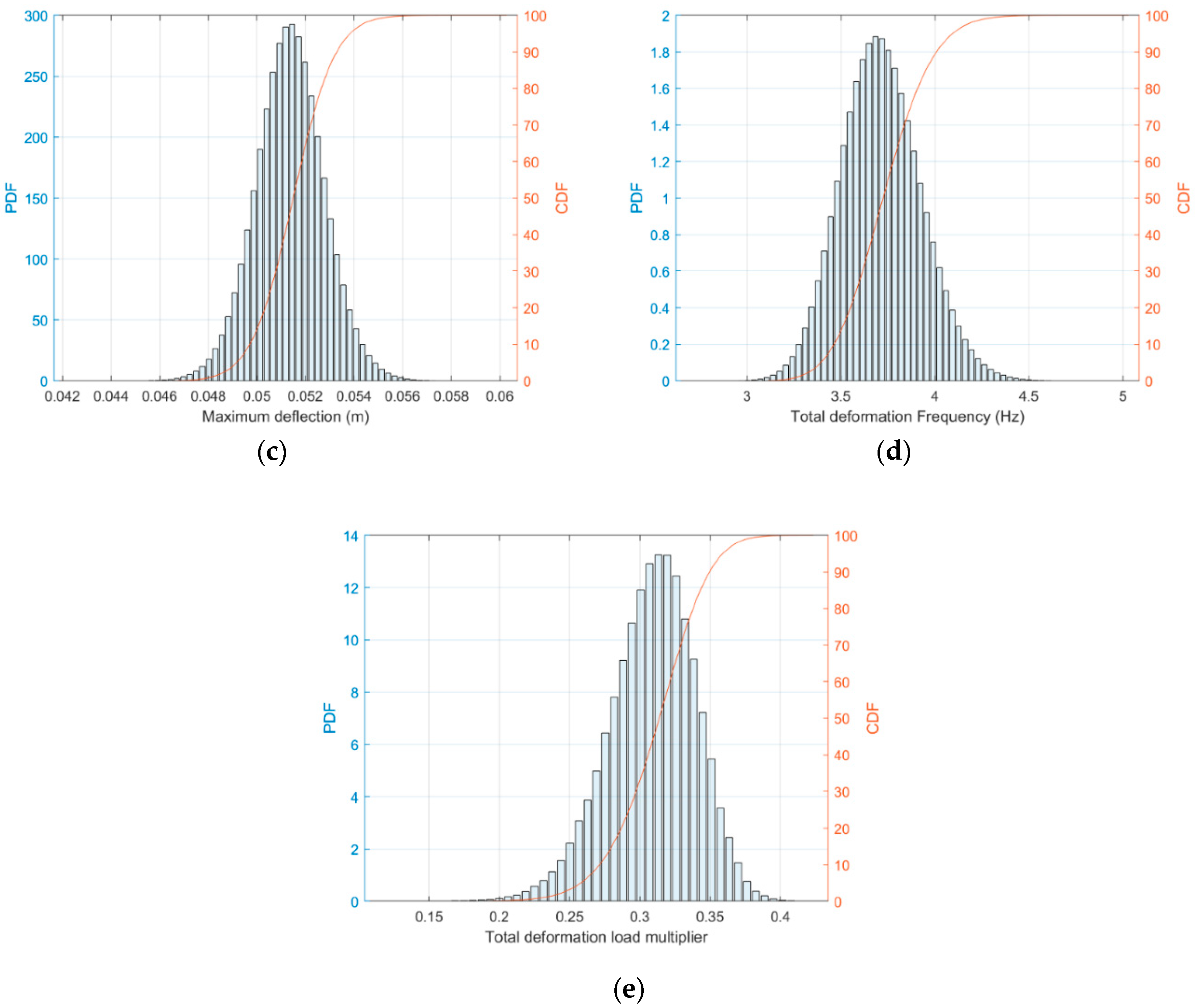
Figure 8a–e depict the probability density function (PDF) histogram and cumulative density function (CDF) of the output parameters for each design constraint from DesignXplorer©.

For the stress constraint case (ULS), the probability that maximum equivalent stress remains less than ${\sigma }_{VM, allow}=323\mathrm{MPa}$, $P_f\left({\sigma }_{VM}\le 323MPa\right)$, is about 0.99999867 which means that there is $1-0.99999867=1.327655\times {10}^{-6}$ probability that the von Mises stress exceed the limit value of 323 MPa, i.e., $P_f\left({\sigma }_{VM}>323MPa\right)=1.327655\times {10}^{-6}$. Therefore, the probability of failure of the critical component of the structure is $1.327655\times {10}^{-6}$ considering the ULS (stress constraint) design criteria. The corresponding reliability index value is $\beta =4.7$.

For the fatigue constraint case (FLS), the probability that the minimum safety factor is less than $f_{sr,allow}=1.15$, $P_f\left(f_{sr}\le 1.15\right)$, is about $5.6461\times {10}^{-7}$. Therefore, the probability of failure of the critical component of the structure is $5.6461\times {10}^{-7}$ considering FLS design criteria (using time-invariant analysis). The corresponding reliability index value is $\beta =4.87$.

For the deformation constraint (SLS), the DesignXplorer© simulation could not produce results within the region of $P_f\left(d\le 0.54\right)$, i.e., $d_{allow}=0.54$. The value $P_f\left(d>0.54\right)$, which is the value of the probability of failure, is expected to be very small, and this is identified as a limitation of the direct MCS requiring a prohibitively large number of simulations to estimate results of this magnitude. Similarly, for the buckling constraint case (ULS), the simulation could not produce the results within the region of $P_f\left(L_m\le 1.4\right)$, as this value is expected also to be very small.

For the vibration constraint (SLS), the probability of failure of the critical component of the structure $P_f\left(f_{1st}\le 0.133\right)$ is about $0.1276\times {10}^{-4}$, and the corresponding $\beta =4.21$.

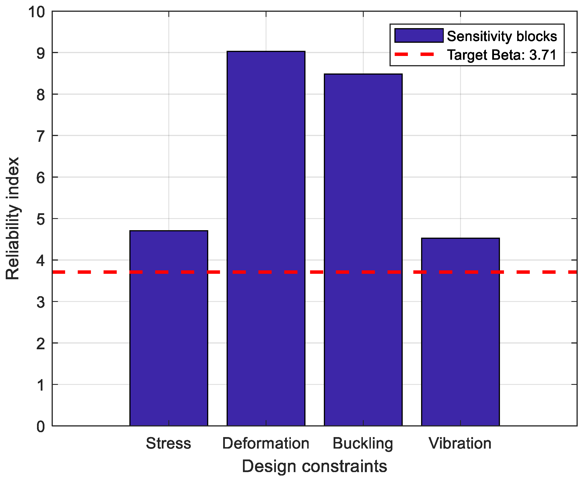
The results obtained from the non-intrusive formulation for each design constraint are depicted in Figure 9 and

Table 10. Computed probability of failure and safety index values using first-order reliability method (FORM) for different limit states.

Design Constraint	Computed Probability of Failure	Computed Safety Index
Stress constraint (ULS)	$0.127\times {10}^{-5}$	4.706
Deflection constraint (SLS)	$0.869\times {10}^{-19}$	9.030
Buckling constraint (ULS)	$0.113\times {10}^{-16}$	8.481
Vibration constraint (SLS)	$0.570\times {10}^{-5}$	4.389

. The results obtained from a time-invariant fatigue reliability assessment employing the FORM are the reliability index, $\beta =5.077$, and probability of failure, $P_f=0.192\times {10}^{-6}$.

As evident from the results above, the reliability assessment performed on the structure shows that the present model, as designed and for the modeling of the stochastic variables considered, satisfies the recommended reliability assessment criteria, as the reliability indices for all the design constraints considered are within the design thresholds. The target reliability index for OWT support structures is typically 3.71, corresponding to a probability of failure of ${10}^{-4}$ according to the DNV [91].

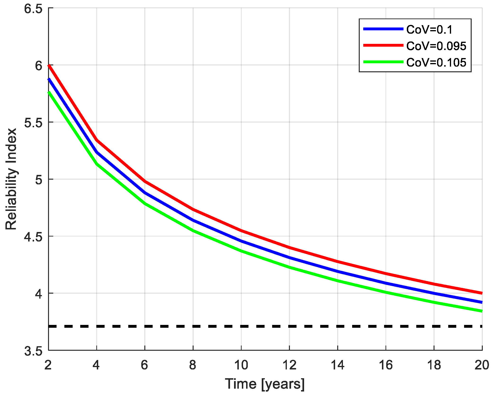
In this work, the time-variant fatigue reliability assessment was carried out using the fatigue analysis guidelines in the DNV standard [71,92], and this is presented in Figure 10. In this study, the thickness-corrected cathodic-protected D curve given by DNV-OS-J101 [71] is chosen for fatigue analysis. The intercept (A) and slope (m) of the S-N curve used for studying the fatigue life of steel structure in seawater for $N>{10}^6$ are given as 15.606 and 5, respectively. From the time-variant fatigue reliability index curve, it can be observed that the structure maintains a reliability index of $3.92$, exceeding the defined threshold of target reliability as specified by DNV for the nominal 20 years of operation. It can be observed that the fatigue limit state dominates the design of OWT support structures, as the reliability index for the fatigue limit state is lower than other reliability index values (see the time-variant fatigue reliability assessment at time = 20 years).

As observed in

Table 11. Comparison between the reliability index values computed by the two methods.

Design Constraint/Limit State	Reliability Index (ANSYS)	Reliability Index (Non-Intrusive Formulation)	Percentage Difference (%)
Stress constraint (ULS)	4.696	4.706	−0.21%
Fatigue constraint (FLS) (time-invariant analysis)	4.870	5.077	−4.25%
Deformation constraint (SLS)	-	9.030
Buckling constraint (ULS)	-	8.727
Vibration constraint (SLS)	4.211	4.389	−4.23%

, the values of safety index, $\beta$, predicted by the non-intrusive reliability analysis formulation were marginally higher than those predicted by the ANSYS probabilistic analysis for the different design constraints. However, the difference in the predicted reliability index values from both methods remains consistently below 5%; hence, the agreement of the two methods can be considered sufficient. Furthermore, considering the observed time required, the FORM simulations run instantly compared to the LHS (as packaged in the ANSYS DesignXplorer©), which requires about 15 min to run on a high-performance computer (i.e., for the 1 × 10⁷ samples).

Additionally, a case study is performed to investigate the effects of COV of the stochastic variables on the fatigue reliability index. In this case, two additional values of COV are considered, i.e., a 5% increase and 5% decrease. The calculated fatigue reliability index over 20-year service life with different values of COV is depicted in Figure 11. As can be seen from Figure 11, the reliability index is sensitive to the value of COV. The higher value of COV means higher uncertainties in stochastic variables, resulting in lower reliability.

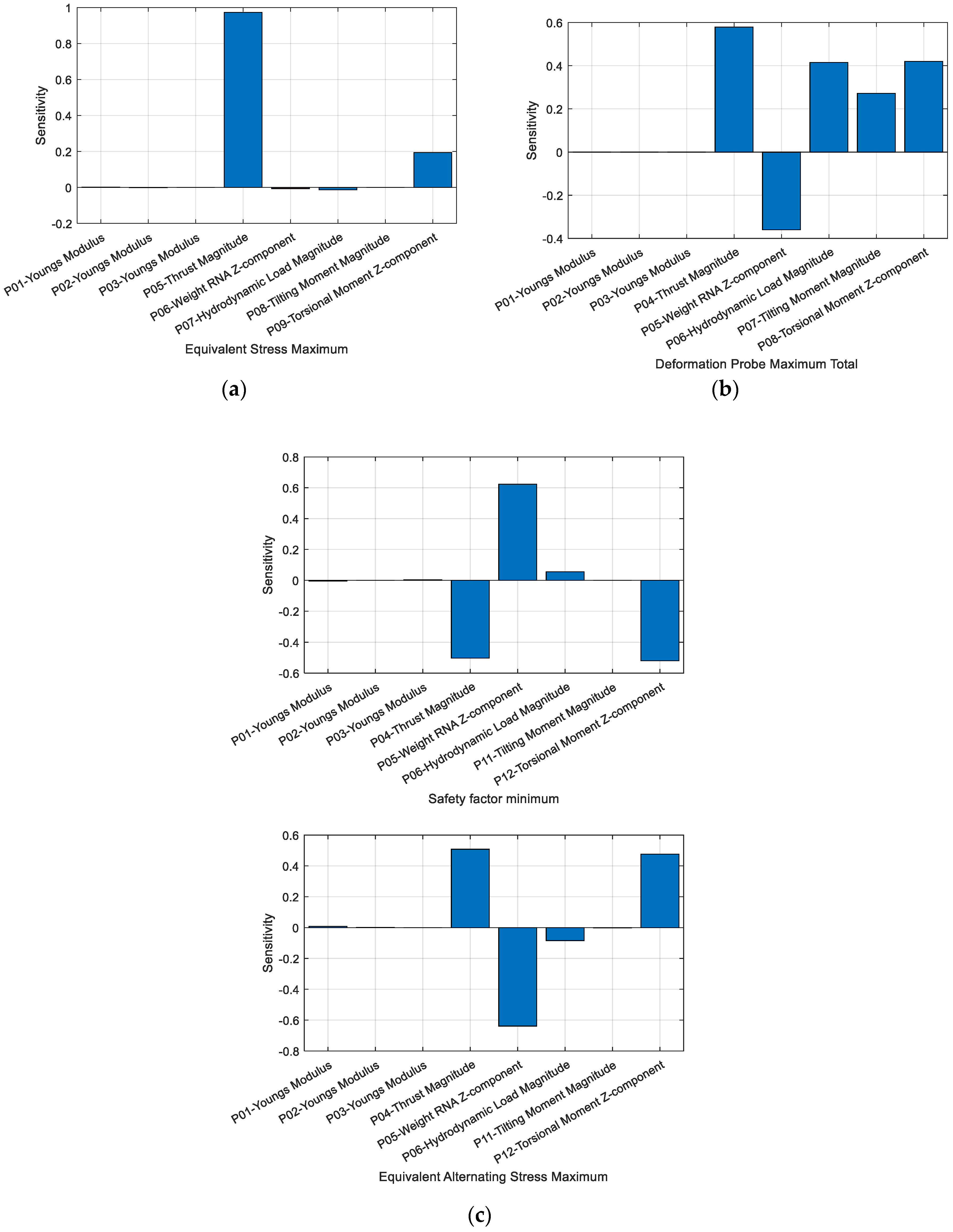
A global sensitivity analysis is also presented from the ANSYS probabilistic analysis for each of the design constraints through post-processing the results. These depict the most critical and important parameters that can radically change the response and reliability performance of the structure. Figure 12a–e show how sensitive the input design variables are to the structure based on the different design criteria. The bar heights indicate sensitivity in these charts.

In Figure 12a, for the probability distribution of the maximum equivalent von Mises stress, it can be observed that the thrust magnitude and the torsional moment are positively correlated with direct impact. The RNA weight and the hydrodynamic load are negatively correlated and have little influence but inversely. The Young’s modulus of the soil system and the tilting moment are neutral and have limited or no impact.

In Figure 12b, for the probability distribution of the deformation at the jacket top, it can be observed that four variables are positively correlated with direct impact. These are the thrust load, hydrodynamic load, and tilting and torsional moments, which have significant influence. The Young’s modulus of the soil system has little or no impact. The RNA weight is negatively correlated and has a significant impact.

In Figure 12c, for the probability distribution of the minimum output parameter safety factor, it can be observed that Young’s modulus of the soil system is neutral and has little or no impact. The RNA weight and hydrodynamic load are positively correlated with direct impact; the RNA weight has significant influence while the hydrodynamic load has quite some impact. The thrust and the torsional moments are negatively correlated and have significant influence but inversely. The tilting moment has very little or no impact.

As can be seen from Figure 12d, the RNA weight and the thrust load have the highest impact and are positively and negatively correlated, respectively, with the other variables having little or no impact on the load multiplier probability distribution. It can also be observed that, in Figure 12e, the structure self-weight has the highest direct impact, with the thrust load and the second soil strata having very little inverse impact on the distribution of the output parameter, the first eigen-frequency, and, hence, the reliability of the structure.

8. Conclusions

In this study, a comparative analysis on the structural reliability of an OWT support structure between a commercial package and a purpose-developed, non-intrusive stochastic formulation was presented. Both methods start by defining the limit states taking account of the various design constraints. The design constraints considered in this study were as follows: stress (ULS), fatigue (FLS), deformation (SLS), buckling (ULS), and vibration (SLS). A 3D (three-dimensional) parametric FEA (finite element analysis) model of a typical OWT jacket-type support structure was developed, taking account of soil-structure interaction and stochastic variables (i.e., soil properties, wind, wave, and current loads). The series of FEA simulation results were post-processed using two methods. In the first method, the design of experiment and response surface module in the DesignXplorer© were used in order to map the response domain and then derive an appropriate response surface model. The probabilistic assessment was performed using the six sigma analysis function employing the Latin hypercube sampling method in computing the probability of failure, which was then translated to a reliability index. In the second method, multivariate quadratic regression was employed to derive the performance function expressed in terms of global stochastic variables using results from the FEA simulations. Next, FORM was employed to calculate the reliability index and then the probability of failure.

The following conclusions can be drawn from the present study:

• The two methods, i.e., the probabilistic tool package in ANSYS and the developed non-intrusive formulation, match well on the calculated reliability indices calculated for all limit states, cross-verifying applicability of both methods for the structural reliability assessment of OWT support structures.
• The proposed non-intrusive formulation for SRA allows faster calculations, assessment of time-variant fatigue reliability assessment, and calculation of low values of probability of failure in complex engineering systems such as offshore and marine structures.
• This study also allowed for verification of the non-intrusive formulation, which can allow multiple problems of complex nature to be solved probabilistically, alleviating the need for an integrated, application-specific tool to be developed, instead of with the proposed modular formulation.

References

1. Kolios, A.; Wang, L. Advanced Reliability Assessment of Offshore Wind Turbine Monopiles by Combining Reliability Analysis Method and SHM/CM Technology. In Proceedings of the 28th International Ocean and Polar Engineering Conference, Sapporo, Japan, 10–15 June 2018; pp. 1412–1419. [Google Scholar]
2. Wang, L.; Kolios, A. A Generic Framework for Reliability Assessment of Offshore Wind Turbine Monopiles Considering Soil-Solid Interaction and Harsh Marine Environments. In Proceedings of the 5th International Conference on Marine Structures, MARSTRUCT, Lisbon, Portugal, 8–10 May 2017. [Google Scholar]
3. EWEA. EWEA Offshore Wind in Europe—Walking the Tightrope to Success; The European Wind Energy Association: Brussels, Belgium, 2015. [Google Scholar]
4. Ioannou, A.; Angus, A.; Brennan, F. A lifecycle techno-economic model of offshore wind energy for different entry and exit instances. Appl. Energy 2018, 221, 406–424. [Google Scholar] [CrossRef]
5. Damiani, R.; Song, H. A Jacket Sizing Tool for Offshore Wind Turbines within the Systems Engineering Initiative. In Proceedings of the Offshore Technology Conference, Houston, TX, USA, 6–9 May 2013. [Google Scholar]
6. Wang, X.; Zeng, X.; Yang, X.; Li, J. Feasibility study of offshore wind turbines with hybrid monopile foundation based on centrifuge modeling. Appl. Energy 2018, 209, 127–139. [Google Scholar] [CrossRef]
7. Wang, X.; Zeng, X.; Yang, X.; Li, J. Seismic response of offshore wind turbine with hybrid monopile foundation based on centrifuge modelling. Appl. Energy 2019, 235, 1335–1350. [Google Scholar] [CrossRef]
8. Damiani, R.R.; Song, H.; Robertson, A.N.; Jonkman, J.M. Assessing the Importance of Nonlinearities in the Development of a Substructure Model for the Wind Turbine CAE Tool FAST. In ASME 2013 32nd International Conference on Ocean, Offshore and Arctic Engineering; American Society American Society of Mechanical Engineers Digital Collection: New York, NY, USA, 2013; Volume 8. [Google Scholar]
9. Oyvind, N.S. Offshore Wind Turbine. Patent No: US 2011/0311360 A1, 10 February 2009. [Google Scholar]
10. Nielsen, F.G. Wind Turbine for Use Offshore. Patent No: US 7,456,515 B2, 25 November 2008. [Google Scholar]
11. Fyfe, A.J. Support Structure for An Offshore Wind Turbine. Patent No: US 2013/0183163 A1, 13 July 2013. [Google Scholar]
12. Li, F.; Niu, F.; Kang, Z.; Meiyang, Z.; Zhu, R. Jacket Platform of Offshore Wind Turbine. Patent No: CN103669312A, 26 March 2014. [Google Scholar]
13. Lee, J.K. Supporting Structure for Offshore Wind Power System. Patent No: KR20130076251A, 8 July 2003. [Google Scholar]
14. Kidu, K. Transition Pieces of Offshore Wind Turbines and Whole Structure of Wind Turbines Having it. Patent No: KR101613844B1, 7 July 2015. [Google Scholar]
15. Pipee, A.J. Support Structure for An Offshore Wind Turbine. Patent No: KR101786063B1, 27 July 2012. [Google Scholar]
16. Hyun, K.D.; Yun, J.-L.; Keun, L.S. Reliability Analysis Method for Offshore Wind Turbine Support Structure Recording Medium for the Same and Electronic Device Comprising the Same. Patent No: KR101562457B1, 12 October 2015. [Google Scholar]
17. Fischer, T.; Soe-Jensen, A. Monopile Foundation for Offshore Wind Turbine. Patent No: WO2009026933A1, 29 August 2008. [Google Scholar]
18. Park, G. One Body Type Jacket Support Structure for Offshore Wind Turbine. Patent No: KR101865511B1, 4 July 2017. [Google Scholar]
19. Kolios, A.; Di Maio, L.F.; Wang, L.; Cui, L.; Sheng, Q. Reliability assessment of point-absorber wave energy converters. Ocean Eng. 2018, 163, 40–50. [Google Scholar] [CrossRef]
20. Leimeister, M.; Kolios, A. A review of reliability-based methods for risk analysis and their application in the offshore wind industry. Renew. Sustain. Energy Rev. 2018, 91, 1065–1076. [Google Scholar] [CrossRef]
21. Wang, L.; Liu, X.; Renevier, N.; Stables, M.; Hall, G.M. Nonlinear aeroelastic modelling for wind turbine blades based on blade element momentum theory and geometrically exact beam theory. Energy 2014, 76, 487–501. [Google Scholar] [CrossRef]
22. Petrini, F.; Manenti, S.; Gkoumas, K.; Bontempi, F. Structural Design and Analysis of Offshore Wind Turbines from a System Point of View. Wind Eng. 2010, 34, 85–107. [Google Scholar] [CrossRef] [Green Version]
23. Wang, L.; Kolios, A.; Nishino, T.; Delafin, P.L.; Bird, T. Structural optimisation of vertical-axis wind turbine composite blades based on finite element analysis and genetic algorithm. Compos. Struct. 2016, 153, 123–138. [Google Scholar] [CrossRef] [Green Version]
24. Gentils, T.; Wang, L.; Kolios, A. Integrated structural optimisation of offshore wind turbine support structures based on finite element analysis and genetic algorithm. Appl. Energy 2017, 199, 187–204. [Google Scholar] [CrossRef] [Green Version]
25. Wang, L.; Quant, R.; Kolios, A. Fluid structure interaction modelling of horizontal-axis wind turbine blades based on CFD and FEA. J. Wind Eng. Ind. Aerodyn. 2016, 158, 11–25. [Google Scholar] [CrossRef] [Green Version]
26. Achmus, M.; Abdel-Rahman, K. Finite Element Modelling of Horizontally Loaded Monopile Foundations for Offshore Wind Energy Converters in Germany. In Proceedings of the International Symposium on Frontiers in Off-shore Geotechnics (ISFOG), Perth, Australia, 19–21 September 2005. [Google Scholar]
27. Wang, L.; Kolios, A.; Delafin, P.-L.; Nishino, T.; Bird, T. Fluid structure interaction modelling of a novel 10MW vertical-Axis Wind Turbine Rotor Based on Computational Fluid Dynamics and Finite Element Analysis. In Proceedings of the EWEA 2015 Annual Event, Paris, France, 17–20 November 2015; Volume 44. [Google Scholar]
28. Jung, S.; Kim, S.R.; Patil, A.; Hung, L.C. Effect of monopile foundation modeling on the structural response of a 5-MW offshore wind turbine tower. Ocean Eng. 2015, 109, 479–488. [Google Scholar] [CrossRef] [Green Version]
29. DNV GL AS. Standard DNVGL-ST-0126—Support Structures for Wind Turbines; DNV GL: Oslo, Norway, 2016; pp. 1–182. [Google Scholar]
30. Sørensen, J.D. Reliability-Based Calibration of Fatigue Safety Factors for Offshore Wind Turbines. In Proceedings of the Twenty-First International Offshore and Polar Engineering Conference, Maui, HI, USA, 19–24 June 2011. [Google Scholar]
31. Márquez-Domínguez, S.; Sørensen, J.D. Fatigue Reliability and Calibration of Fatigue Design Factors for Offshore Wind Turbines. Energies 2012, 5, 1816–1834. [Google Scholar] [CrossRef] [Green Version]
32. Morató, A.; Sriramula, S.; Krishnan, N. Reliability Analysis of OffshoreWind Turbine Support Structures Using Kriging Models. In Risk, Reliability and Safety: Innovating Theory and Practice; Walls, L., Revie, M., Bedford, B., Eds.; Taylor & Francis Group: London, UK, 2017. [Google Scholar]
33. Wei, K.; Arwade, S.R.; Myers, A.T. Incremental wind-wave analysis of the structural capacity of offshore wind turbine support structures under extreme loading. Eng. Struct. 2014, 79, 58–69. [Google Scholar] [CrossRef]
34. Kim, D.H.; Lee, S.G. Reliability analysis of offshore wind turbine support structures under extreme ocean environmental loads. Renew. Energy 2015, 79, 161–166. [Google Scholar] [CrossRef]
35. Mardfekri, M.; Gardoni, P. Probabilistic demand models and fragility estimates for offshore wind turbine support structures. Eng. Struct. 2013, 52, 478–487. [Google Scholar] [CrossRef]
36. Mardfekri, M.; Gardoni, P. Multi-hazard reliability assessment of offshore wind turbines. Wind Energy 2015, 18, 1433–1450. [Google Scholar] [CrossRef] [Green Version]
37. Vahdatirad, M.J.; Griffiths, D.; Andersen, L.V.; Sørensen, J.D.; Fenton, G. Reliability analysis of a gravity-based foundation for wind turbines: A code-based design assessment. Géotechnique 2014, 64, 635–645. [Google Scholar] [CrossRef]
38. Yeter, B.; Garbatov, Y.; Soares, C.G. Fatigue reliability of an offshore wind turbine supporting structure accounting for inspection and repair. In Analysis and Design of Marine Structures; Soares, G., Shenoi, E., Eds.; Taylor & Francis Group: London, UK, 2015; pp. 737–747. [Google Scholar]
39. Yeter, B.; Garbatov, Y.; Soares, C.G. Reliability of Offshore Wind Turbine Support Structures Subjected to Extreme Wave-Induced Loads and Defects. In Proceedings of the ASME 2016 35th International Conference on Ocean, Offshore and Arctic Engineering OMAE2016-54240, Busan, Korea, 30 June 2016; pp. 1–8. [Google Scholar]
40. Yeter, B.; Garbatov, Y.; Guedes Soares, C. System Reliability of a Jacket Offshore Wind Turbine Subjected to Fatigue. In Proceedings of the 5th International Conference on Marine Structures, MARSTRUCT, Lisbon, Portugal, 8–10 May 2017; pp. 939–950. [Google Scholar]
41. Yeter, B.; Garbatov, Y.; Guedes Soares, C. Uncertainty analysis of soil-pile interactions of monopile offshore wind turbine support structures. Appl. Ocean Res. 2019, 82, 74–88. [Google Scholar] [CrossRef]
42. Dong, W.; Moan, T.; Gao, Z. Fatigue reliability analysis of the jacket support structure for offshore wind turbine considering the effect of corrosion and inspection. Reliab. Eng. Syst. Saf. 2012, 106, 11–27. [Google Scholar] [CrossRef]
43. Muskulus, M.; Schafhirt, S. Reliability-Based Design of Wind Turbine Support Structures. In Proceedings of the Symposium on Reliability of Engineering System, Hangzhou, China, 2–5 November 2015. [Google Scholar]
44. Ciampoli, M.; Petrini, F. Performance-based design of offshore wind turbines. In Earth and Space 2010: Engineering, Science, Construction, and Operations in Challenging Environments; American Society of Civil Engineers: Reston, VA, USA, 2010. [Google Scholar]
45. Karadeniz, H. Review of Structural Reliability Methods with Applicability in Practice. Civ. Eng. 2006, 4, 880653. [Google Scholar]
46. Choi, S.-K.; Grandhi, R.; Canfield, R. Reliability-based Structural Design; Springer: Berlin/Heidelberg, Germany, 2006. [Google Scholar]
47. Bai, Y. Marine Structural Design, 1st ed.; Elsevier: Amsterdam, The Netherlands, 2003. [Google Scholar]
48. Ang, A.; Tang, W. Probability concepts in engineering planning and design. In Decision, Risk, and Reliability; John Wiley Sons: New York, NY, USA, 1984; Volume 2. [Google Scholar]
49. Kolios, A. A Multi-Configuration Approach to Reliability Based Structural Integrity Assessment for Ultimate Strength. Ph.D. Thesis, Cranfield University, Bedford, UK, 2010. [Google Scholar]
50. Hohenbichler, M.; Rackwitz, R. First-order conceepts in structural reliability. Struct. Saf. 1983, 1, 177–188. [Google Scholar] [CrossRef]
51. Der Kiureghian, A.; Lin, H.-Z.; Hwang, S.-J. Second Order Reliability Approximations. J. Eng. Mech. Div ASCE 1987, 113, 1208–1225. [Google Scholar] [CrossRef]
52. Jiang, Z.; Hu, W.; Dong, W.; Gao, Z.; Ren, Z. Structural reliability analysis of wind turbines: A review. Energies 2017, 10, 2099. [Google Scholar] [CrossRef] [Green Version]
53. ANSYS DesignXplorer User’s Guide. 2018. Available online: www.ansys.com (accessed on 1 April 2018).
54. Reh, S.; Beley, J.D.; Mukherjee, S.; Khor, E.H. Probabilistic finite element analysis using ANSYS. Struct. Saf. 2006, 28, 17–43. [Google Scholar] [CrossRef]
55. Melchers, R.; Andre, T. Structural Reliability Analysis and Prediction, 3rd ed.; Wiley: Hoboken, NJ, USA, 2018. [Google Scholar]
56. Melchers, R.E. Structural Reliability: Analysis and Prediction, 2nd ed.; Ellis Horwood: Chichester, UK, 2002. [Google Scholar]
57. Hammersley, J.M.; Handscomb, D.C. Monte Carlo Methods; Chapman & Hall: London, UK, 1964. [Google Scholar]
58. Mastumoto, M.; Nishimura, T. Mersenne twister: A 623-Dimensionally equidistributed uniform pseudorandom number generator. ACM Trans Model. Comput. Simul. 1998, 8, 3–30. [Google Scholar]
59. Kececioglu, D. Reliability Engineering Handbook; Prentice-Hall: Upper Sadle River, NJ, USA, 1991; Volume 2. [Google Scholar]
60. Ayyub, B.M.; Lai, K.-L. Structural Reliability Assessment Using Latin Hypercube Sampling. In Structural Safety and Reliability, Proceedings of the 5th International Conference on Structural Safety and Reliability (ICOSSAR), San Francisco, CA, USA, 7–11 August 1989; Ang, A.-S., Shinozuka, M., Schueler, G., Eds.; American Society of Civil Engineers: San Francisco, CA, USA, 1989; pp. 1177–1184. [Google Scholar]
61. Florian, A. An efficient sampling scheme: Updated latin hypercube sampling. Probab. Eng. Mech. 1992, 7, 123–130. [Google Scholar] [CrossRef]
62. Ang, A.-S.; Tang, W.H. Probabilistic Concepts in Engineering Planing and Design. Basic Principles; Wiley: New York, NY, USA, 1975. [Google Scholar]
63. Dahlquist, G.; Björck, A. Numerical Methods; Prentice-Hall: Englewood Cliffs, NJ, USA, 1974. [Google Scholar]
64. Rubinstein, R.Y. Simulation and the Monte Carlo Method; John Wiley & Sons: New York, NY, USA, 1981. [Google Scholar]
65. Warner, R.F.; Kabaila, A.P. Monte Carlo study of structural safety. J. Struct. Div. ASCE 1968, 94, 2847–2859. [Google Scholar]
66. McKay, M.; Beckman, R.; Conover, W. A comparison of three methods for selecting values of input variables in the analysis of output from a computer code. Technometrics 1979, 21, 239–245. [Google Scholar]
67. Melchers, R.E. Structural Reliability: Analysis and Prediction, 1st ed.; Ellis Horwood: Chichester, UK, 1999. [Google Scholar]
68. Olsson, A.; Sandberg, G.; Dahlblom, O. On Latin hypercube sampling for structural reliability analysis. Struct. Saf. 2003, 25, 47–68. [Google Scholar] [CrossRef]
69. Huntington, D.E.; Lyrintzis, C.S. Improvements to and limitations of Latin hypercube sampling. Prob. Eng. Mech. 1998, 13, 245–253. [Google Scholar] [CrossRef]
70. Hasofer, A.; Lind, N. An exact and invariant second moment code format. J. Eng. Mech. Div ASCE 1974, 100, 111–121. [Google Scholar]
71. DNV. DNV-OS-J101 Design of Offshore Wind Turbine Structures; DNV GL: Oslo, Norway, 2014; pp. 212–214. [Google Scholar]
72. IEC. Wind Turbines—Part 3: Design Requirements for Offshore Wind Turbines. In Proceedings of the IEC 61400-3, Geneva, Switzerland, 2009. [Google Scholar]
73. Veritas, N. Environmental Conditions and Environmental Loads; DNV GL: Oslo, Norway, 2000. [Google Scholar]
74. Minguez, L. Fatigue and Fracture Mechanics of Offshore Wind Turbine Support Structures. Ph.D. Thesis, Cranfield University, Bedford, UK, 2015. [Google Scholar]
75. Freebury, G.; Musial, W. Determining equivalent damage loading for full-scale wind turbine blade fatigue tests. In Proceedings of the 2000 ASME Wind Energy Symposium, Reno, NV, USA, 10–13 January 2000. [Google Scholar]
76. Chakrabarti, S.K. Handbook of Offshore Engineering; Elsevier: Amsterdam, The Netherlands, 2005; Volume 1. [Google Scholar]
77. Muskulus, M.; Schafhirt, S. Design Optimization of Wind Turbine Support Structures—A Review. J. Ocean Wind Energy 2014, 1, 12–22. [Google Scholar]
78. Lee, Y.S.; Choi, B.L.; Lee, J.H.; Kim, S.Y.; Han, S. Reliability-based design optimization of monopile transition piece for offshore wind turbine system. Renew. Energy 2014, 71, 729–741. [Google Scholar] [CrossRef]
79. IEC. IEC 61400-1: Wind Turbines Part 1: Design Requirements; IEC: Geneve, Switzerland, 2005. [Google Scholar]
80. Fisher, T.; De Vries, W.; Schmidt, B. Upwind Design Basis (WP4 Offshore Foundations and Support Structures). 2010. Available online: https://repository.tudelft.nl/islandora/object/uuid%3Aa176334d-6391-4821-8c5f-9c91b6b32a27 (accessed on 4 June 2019).
81. Schaumann, P.; Boker, C.; Bechtel, A.; Lochte-Holtgreven, S. Support structures of wind energy converters. In Environmental Wind Engineering and Design of Wind Energy Structures; Baniotopoulos, C., Borri, C., Stathopoulos, T., Eds.; Springer: Berlin/Heidelberg, Germany, 2011; pp. 191–253. [Google Scholar]
82. GL Rule for Regulation IV-Non Marine Technology, Part 2 Offshore Wind Energy. 1995. iani, R. In JacketSE: An Offshore Wind Turbine Jacket Sizing Tool Theory Manual and Sample Usage with Preliminary Validation; National Renewable Energy Lab.(NREL): Golden, CO, USA, 2016.
83. Damiani, R. JacketSE: An Offshore Wind Turbine Jacket Sizing Tool Theory Manual and Sample Usage with Preliminary Validation; National Renewable Energy Lab.(NREL): Golden, CO, USA, 2016. [Google Scholar]
84. Jonkman, J.; Butterfield, S.; Musial, W.; Scott, G. Definition of a 5-MW Reference Wind Turbine for Offshore System Development; National Renewable Energy Lab. (NREL): Golden, CO, USA, 2009. [Google Scholar]
85. Drucker, D.; Prager, W. Soil mechanics and plastic analysis or limit design. Q. Appl. Math. 1952, 10, 157–165. [Google Scholar] [CrossRef] [Green Version]
86. ANSYS Inc. Introduction to Contacts—ANSYS Mechanical Structural Nonlinearities; ANSYS Inc.: Canonsburg, PA, USA, 2010. [Google Scholar]
87. ANSYS. ANSYS Help Documentation. 2018. Available online: www.ansys.com (accessed on 5 June 2019).
88. Kühn, M. Dynamics and Design Optimization of Offshore Wind Energy Conversion Systems; DUWIND, Delft University Wind Energy Research Institute: Delft, The Netherlands, 1999. [Google Scholar]
89. Zwick, D. Simulation and Optimization in Offshore Wind Turbine Structural Analysis. Ph.D. Thesis, Norwegian University, Trondheim, Norway, 2015. [Google Scholar]
90. BSI. BS EN 1990 Eurocode: Basis of Structural Design; British Standards Institute: London, UK, 2002. [Google Scholar]
91. (DNV) Det Norske Veritas. Structural Reliability Analysis of Marine Structures; Det Norske Veritas: Oslo, Norway, 1992. [Google Scholar]
92. Det Norske Veritas. Fatigue design of offshore steel structures. In DNV Recommended Practice DNV-RP-C203; Det Norske Veritas: Oslo, Norway, 2010; pp. 37–41. [Google Scholar]
Figure 1. Flow chart of the non-intrusive formulation method [2].
Applsci 10 00860 g001
Figure 2. Representation of the loads on the support structure of the offshore wind turbine (OWT) and jacket geometry embedded in layered soil.
Applsci 10 00860 g002
Figure 3. Mesh convergence test.
Applsci 10 00860 g003
Figure 4. Three-dimensional (3D) display of meshing performed on the structural model.
Applsci 10 00860 g004
Figure 5. The 3D display of structural model with applied loads and boundary conditions.
Applsci 10 00860 g005
Figure 6. Display of structural model’s modal analysis results showing the first mode frequency.
Applsci 10 00860 g006
Figure 7. Display of results of total deformation showing the deflection at the RNA level.
Applsci 10 00860 g007
Figure 8. Cumulative density function (CDF) and histogram for the output parameter: (a) maximum von Mises stress (stress constraint case); (b) fatigue safety factor minimum (fatigue constraint case); (c) maximum deformation; (d) total deformation load multiplier (buckling constraint case);, (e) first eigen-frequency (vibration constraint case)-DesignXplorer©.
Applsci 10 00860 g008aApplsci 10 00860 g008b
Figure 9. Reliability index of different design constraints (non-intrusive formulation).
Applsci 10 00860 g009
Figure 10. Fatigue reliability assessment (non-intrusive formulation).
Applsci 10 00860 g010
Figure 11. Fatigue reliability index with different coefficients of variation (COVs).
Applsci 10 00860 g011
Figure 12. Global sensitivity chart: (a) stress design constraint (ULS); (b) deformation design constraint (SLS); (c) fatigue design constraint; (d) buckling constraint (ULS); (e) vibration constraint (SLS).
Applsci 10 00860 g012aApplsci 10 00860 g012b