Article

Image Super-Resolution Based on CNN Using Multilabel Gene Expression Programming

1
College of Computer Engineering, Jiangsu University of Technology, Changzhou 213001, Jiangsu, China
2
School of Computer Engineering, Nanjing Institute of Technology, Nanjing 211167, Jiangsu, China
*
Author to whom correspondence should be addressed.
Appl. Sci. 2020, 10(3), 854; https://doi.org/10.3390/app10030854
Submission received: 25 December 2019 / Revised: 17 January 2020 / Accepted: 23 January 2020 / Published: 25 January 2020
(This article belongs to the Special Issue Advances in Image Processing, Analysis and Recognition Technology)

Abstract

:
Current mainstream super-resolution algorithms based on deep learning use a deep convolution neural network (CNN) framework to realize end-to-end learning from low-resolution (LR) image to high-resolution (HR) images, and have achieved good image restoration effects. However, as the number of layers in the network is increased, better results are not necessarily obtained, and there will be problems such as slow training convergence, mismatched sample blocks, and unstable image restoration results. We propose a preclassified deep-learning algorithm (MGEP-SRCNN) using Multilabel Gene Expression Programming (MGEP), which screens out a sample sub-bank with high relevance to the target image before image block extraction, preclassifies samples in a multilabel framework, and then performs nonlinear mapping and image reconstruction. The algorithm is verified through standard images, and better objective image quality is obtained. The restoration effect under different magnification conditions is also better.

1. Introduction

Aiming at addressing image degradation during digital image acquisition and processing, Single-Image Super-Resolution (SISR) technology [1,2] enables high-resolution (HR) images to be recovered from low-resolution (LR) ones with high-frequency texture details and edge structure information observations of images to meet people’s image quality needs.
Early reconstruction-based SR methods mainly modeled the acquisition process of low-resolution observation images, used the regularization method to construct the prior constraints of high-resolution images, estimated the HR images from the LR observation images, and finally restored the super-resolution image. The problem turns into an optimization problem of a cost function under a constraint [3]. Learning-based super-resolution restoration technology was first proposed by Freeman [4]. This type of algorithm uses the similarity of different images in high-frequency details to obtain the relationship between the HR and LR images through the algorithm to guide the reconstruction of the output image. Prior knowledge can be obtained through learning, instead of defining the prior knowledge in the model-based reconstruction method.
In recent years, deep learning has been a hot topic in the field of machine learning, and its related theories have attracted widespread attention from researchers. It has been gradually used in the field of image super-resolution reconstruction and has better effects than shallow learning [5,6,7,8,9,10,11,12,13]. The most classic of them is an end-to-end deep learning model, the super-resolution convolution neural network (SRCNN), constructed by a three-layer convolutional neural network proposed by Dong et al. [5]. The image is input after Bicubic preprocessing, and it is trained on LR and HR images in pairs. The gradient descent method continuously adjusts the weights to obtain a mapping from LR to HR. Its simple network structure design and excellent image restoration results created a precedent for deep learning in super-resolution image reconstruction. However, the SRCNN method does not obtain better results when the number of layers in the network is increased. The training convergence rate is slow and it is not suitable for multiscale amplification.
Based on the above problems, we propose an improved deep learning algorithm for Gene Expression Programming (GEP) preclassification. This method uses the GEP multilabeling algorithm to classify the trained image set and select a subset of samples that are related in color and texture feature categories, thereby reducing the complexity of the convolutional neural network parameters. We compare the performance of our approach to that of other state-of-the-art methods and obtain improved objective image quality.

2. Related Work

In recent years, deep learning and artificial intelligence have been widely used in various industries, especially in the field of computer vision, and have achieved better results than traditional methods [14,15]. Using the feed-forward depth network methods of CNN is the mainstream of the current super-resolution reconstruction field after sparse representation. Such methods focus less on the reconstruction speed and more on whether the high-resolution map can be better restored at a large magnification. They have better generalization ability and ability to characterize the high-level characteristics, compared with traditional shallow learning algorithms.

2.1. SRCNN/Fast SRCNN (FSRCNN)

Dong et al. [5] first proposed the use of a convolutional neural network for image super-resolution reconstruction. An LR image was first enlarged to the target size using Bicubic interpolation, and then a nonlinear mapping was performed through a three-layer convolutional network. The obtained results were output as high-resolution images, and good results were obtained. As shown in Figure 1, the network structure design of this method is simple. Compared with previous learning algorithms, it saves a lot of artificial feature extraction steps and post-integration, thus opening up the era of deep CNN super-resolution image processing problems.
After that, Dong et al. [6] improved upon the SRCNN, and the fast SRCNN (FSRCNN) was proposed, which increases the depth of the network and introduces a deconvolution layer to restore features. The deconvolution layer can realize the conversion from low-resolution space to high-resolution space. This feature allows the FSRCNN to directly use the low-resolution image instead of the interpolation result as the network input. Directly using LR images as input can not only reduce the calculation amount of the model, but also avoid the obvious artificial traces introduced by interpolation. FSRCNN offers a great improvement in speed, without any preprocessing, to achieve end-to-end input and output of the network, but the restoration accuracy is somewhat insufficient.

2.2. Sparse-Coding-Based Network (SCN)

The SCN method [9] firstly obtains the sparse prior information of the image through the feature extraction layer, then establishes a feed-forward neural network which can implement sparse encoding and decoding of the image, and finally uses a cascade network to complete the image enlargement. This method can improve the Peak Signal-to-Noise Ratio (PSNR) at a higher magnification, and the algorithm running speed is further improved. Moreover, with the correct understanding of each layer’s physical meaning, the SCN method offers a more principled way to initialize the parameters, which helps to improve optimization speed and quality.

2.3. Very Deep Convolutional Networks for Image Super-Resolution (VDSR)

The ultra-deep super-resolution network proposed by Kim et al. [8] extended the SRCNN from a 3-layer shallow network structure to a 20-layer ultra-deep network, and they concluded that the reconstruction effect will be improved as the number of layers increases. Compared to SRCNN, which only depends on the image context in a small area, VDSR, by exploring more contextual information through a larger receptive field, helps to better restore the detailed structure, especially in super-resolution applications with large magnification factors. In addition, in order to solve the problem of slow convergence in SRCNN, VDSR residual learning was introduced, which greatly increased the learning rate.
VDSR accepts image features of different scales by adjusting the size of the filter to produce a fixed feature output. Although VDSR can achieve specific-scale magnification, it cannot achieve free-scale, multiscale magnification, and its parameter storage and retrieval also have obvious shortcomings.

3. The Proposed Method

3.1. Multifeature Representation of Images

Image features include color, texture, shape, and spatial relationships. Features can be extracted from the image after being detected by the computer. The result is called a feature description or feature vector. In this paper, the Multilabel Gene Expression Programming (MGEP) algorithm mainly uses image color and texture features for multilabel recognition.

3.1.1. Color Feature

The color feature is a global feature that describes the surface properties of the scene corresponding to the image or image area, and is also the most direct visual feature in the physical characteristics of the image. Compared with various other image features, the color feature has two obvious advantages: one is stability, low sensitivity to various changes in the image such as translation, scaling, rotation, etc., and strong robustness; the second is that its complicated calculation degree is low. The pixel values in the image are converted, and the corresponding numerical expression is used to obtain the image characteristics [16]. Because of the stability and simple calculation, the color feature has become a widely used image feature.
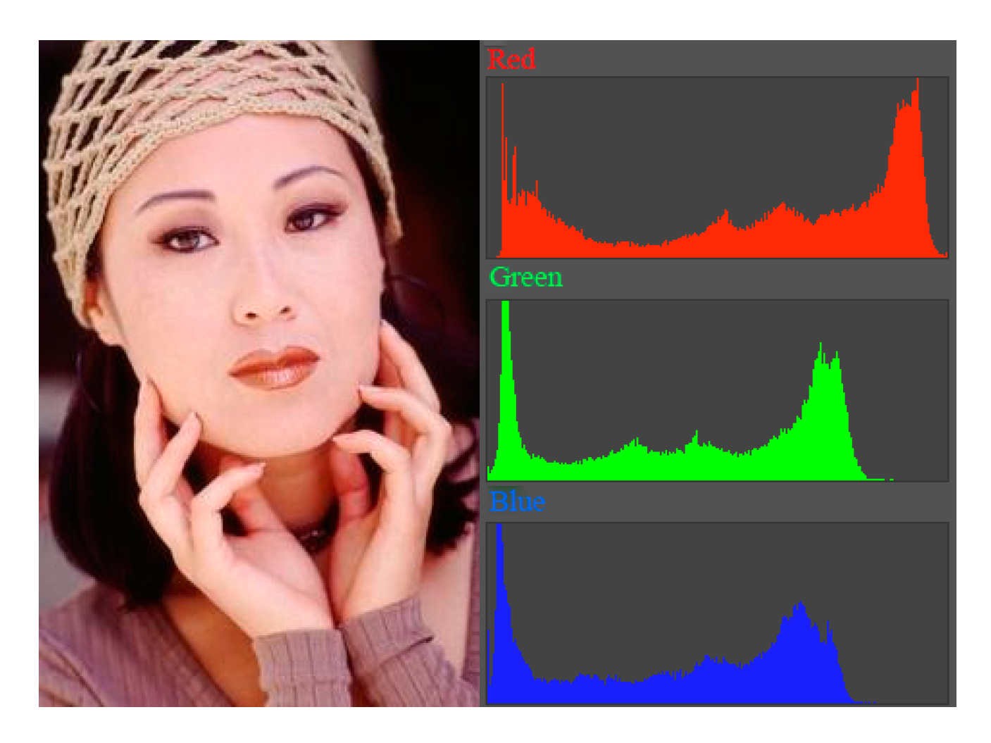
Shown in Figure 2, the color histogram is widely used in many image retrieval systems. It describes the proportion of different colors in the entire image, and does not pay attention to the spatial location of each color; that is, it cannot describe the objects or objects in the image.
The color histogram can be defined as the joint probability density function of the three color channels (RGB) in the image:
h R , G , B ( a , b , c ) = N P ( R = a , G = b , B = c )
where R, G, and B represent the RGB color channels of the image, N indicates the number of image pixels, P represents the probability density function, and h represents a histogram function, defined as a four-dimensional eigenvector H ( H R , H G , H B , μ ) . The first three dimensions HR, HG, and HB correspond to the three color channels, and the last dimension μ indicates the proportion of the color in the entire image.

3.1.2. Texture Feature

Texture is a visual feature that reflects homogeneous phenomena in an image, and it reflects the surface structure organization and arrangement properties of an object surface with slow or periodic changes. Texture is a pattern produced by the gray or color of the target image in space in a certain form [17]. From the perspective of texture, the image can be roughly divided into three cases: first, the gray distribution has a certain periodicity (even if the gray change is random, it also has certain statistical characteristics, and may be in a larger area repeatedly); second, the basic components that make up the sequence are regular rather than random; third, the texture of each part in the texture area shows roughly the same size, structure, and image, and is uniformly distributed as a whole.
The Fourier power spectrum method is used to measure the texture characteristics of the image. Let the texture image be f(x, y); its Fourier transform can be expressed by Equation (2).
F ( u , v ) = f ( x , y ) exp { j 2 π ( u x + v y ) } d x d y
The definition of the power spectrum of the two-dimensional Fourier transform is shown in Equation (3):
| F | 2 = F F
where F* stands for the conjugate of F. The power spectrum | F | 2 reflects the nature of the entire image. If the Fourier transform is expressed in polar form, i.e., F ( r , θ ) form, then the energy on the circle r from the origin is
Φ r = 0 2 π [ F ( r , θ ) ] 2 d θ .
From research on the energy in the small fan-shaped region in the angle θ direction, the law of this energy changing with the angle can be obtained by Equation (5):
Φ θ = 0 | F ( r , θ ) | 2 d r .
When a texture image runs along θ and there are many lines, edges, etc., in the direction θ + π 2 , i.e., in a right-angle direction to θ , the energy is concentrated. If the texture does not show directionality, there is no directionality in the power spectrum. Therefore, the | F | 2 value reflects the directionality of the texture.

3.2. GEP Network

Gene Expression Programming (GEP) was proposed by Ferreira in 2001. It is a new evolutionary model and belongs to the family of genetic algorithms [18,19]. The GEP algorithm, like the Genetic Algorithm (GA) and Genetic Programming (GP), is a computational model that simulates the evolutionary process of living things. Because GEP chromosomes are simple, linear, and compact; make it easy to carry out genetic operations, etc.; and have stronger problem-solving capabilities, they are 2 to 4 orders of magnitude faster than GA and GP [19]. Because of these advantages, GEP technology has attracted the attention of many researchers and has been used in machine learning fields such as function discovery, symbol regression, classification, clustering, and association rule analysis.
( S , F , T ) represents a GEP gene as a 3-tuple, of which S is a fixed-length string, F is the set of calculation functions, and T is the basic terminal set. Sometimes, for convenience, the fixed-length string S is called a gene. The gene is divided into two parts, the head and the tail. The former symbol can be taken from F and T, and the latter must be taken from T. GEP gene coding rules ensure that it can be decoded into an expression tree corresponding to a legal mathematical expression. Suppose its head length is h, tail length is t, and nmax is the maximum number of parameters of a function in the function set; then the relationship between h and t can be expressed by Equation (6).
t = h ( n max 1 ) + 1
GEP’s neural network selective integration process is divided into two stages.
Stage 1: Network group generation.
We use existing methods such as Boosting and Bagging to generate network groups. Assume the output vector of the network population is Y = ( y 1 , y 2 , , y n ) , y i { 0 , 1 } .
Stage 2: Individual network selection and conclusion generation based on GEP.
For input x, there are the following integrated classification results:
y ( x ) = sign ( f ( Y ) ) .
Among them, Y Y , Y = ( y i 1 , y i 2 , , y i m ) . That is, the final classification result is synthesized from some network outputs in the network group in some way. Because GEP has powerful function discovery and parameter selection functions, it can be discovered using the GEP method f(Y′).
Taking the threshold lamda = 0.5, the integrated classification result y(x) is calculated as follows:
y ( x ) = { 1 f ( Y ) 0.5 0 f ( Y ) < 0.5

3.3. Fitness Function Design

The fitness function is the guideline for the evolution of the GEP algorithm. For feed-forward neural networks, the topology selection and training of weights can be regarded as an optimization process. The purpose of optimization is to design the network so that the fitness function value reaches the maximum value. The performance of the current network for a given training data set is described by a least squares error function.
We use category-based multilabel evaluation indicators. We first measure the classifier’s corresponding two-class classification performance on a single class, and then calculate the average performance of the classifier on all classes as the evaluation index value of the classifier. Suppose we have a multilabeled test set with p-many sample data S = { ( x i , Y i ) | 1 i p } for the jth category yj (1 ≤ jq). In terms of the multilabel classifier, the two-class classification performance of h(·) in this category can be described by the four statistics given by Equations (9)–(12).
1. TPj (#true positive instances)
TPj = | {xi | yjYi ˄ yjh(xi), (xi, Yi) ∈ S} |
2. FPj (#false positive instances)
FPj = | {xi | yjYi ˄ yjh(xi), (xi, Yi) ∈ S} |
3. TPj (#true negative instances)
TPj = | {xi | yjYi ˄ yjh(xi), (xi, Yi) ∈ S} |
4. FPj (#false negative instances)
FPj = | {xi | yjYi ˄ yjh(xi), (xi, Yi) ∈ S}|
From Equations (9)–(12), TPj + FPj + TNj + FNj = p is established. Most classification performance indicators, such as accuracy, precision, and recall, can be derived from the above four statistics—see Equations (13)–(15).
Accuracy = B ( T P j ,   F P j ,   T N j ,   F N j )   =   T P j + T N j T P j + F P j + T N j + F N j
Precision = B ( T P j ,   F P j ,   T N j ,   F N j )   =   T P j T P j + F P j
Recall = B ( T P j ,   F P j ,   T N j ,   F N j )   =   T P j T P j + F N j
Therefore, combined with category-based multilabel classification evaluation index, we design a fitness function for the MGEP classification algorithm.
1. Design of fitness function based on macro-averaging:
F i t i = | R 100 × 1 q j = 1 q B ( T P j , F P j , T N j , F N j ) |
2. Design of fitness function based on micro-averaging:
F i t i = | R B ( j = 1 q T P j , j = 1 q F P j , j = 1 q T N j , j = 1 q F N j ) |
In Equations (16) and (17), Fiti is the fitness value of the ith individual to the environment, and R is the selected bandwidth.

3.4. MGEP Classification before CNN Image Super-Resolution

In the process of image super-resolution reconstruction, the traditional K-means clustering algorithm [20] is used to classify the trained image set to improve the training effect and reduce the training time. In the K-means clustering algorithm, the value of K needs to be determined in advance, and it cannot be changed during the entire course of the algorithm, which makes it difficult to accurately estimate the value of K when training high-dimensional data sets.
We used the MGEP classification algorithm instead of the K-means clustering algorithm, and its preclassification model is shown in Figure 3.
Let p-many sample pattern pairs (xk, yk) constitute the training set, k = 1, 2, …, p. According to the definition of the GEP classifier, for sample k, there are xk = (xk1, xk2, …, xkm) and yk = (yk1, yk2, …, ykn), where xkj is the sample in the attribute Aj (j = 1, 2, …, m) and yki is the degree of membership of the sample to the category Ci (i = 1, 2, …, n). The training set constitutes the set of adaptive instances, and the set of adapted instances of a particular problem forms the adaptive environment of the MGEP algorithm. Under a certain adaptive environment, starting from the initial population, selection, replication, and various genetic operations are performed according to individual fitness to form a new population. This process is repeated until the optimal individual is evolved and decoded to obtain a GEP multilabel classifier. In the MGEP preclassification learning, we find similar samples for LR image blocks in terms of color and texture features, thereby shortening the time of the next precise matching and improving the efficiency and effect of SR image restoration.
In the training of the CNN, the MGEP algorithm is used to classify the trained image set, classify the approximate images into one category, and reduce the parameter scale of the convolutional neural network model, which can reduce the training time of the network to a certain extent and improve the training efficiency of the CNN. The improved algorithm flow based on SRCNN is shown in Figure 4.
The algorithm uses Wiener filtering to construct a deconvolution layer, which is used to implement multiscale image reconstruction. The deconvolution network part adopts the mirror structure of the convolution network. The purpose is to reconstruct the shape of the input target, so the multilevel deconvolution structure can also capture the shape details of different levels like the convolution network. In the model of the convolutional network, low-level features can describe the rough information of the entire target, such as target position and approximate shape, while more complex high-level features have classification characteristics and also contain more detailed target information.

4. Experiments

4.1. Experimental Environment and Parameter Settings

The experimental software environment used was Ubuntu 14.04, Python 2.7, TensorFlow 1.4; the hardware environment was an Intel Core i7-6700K, RAM 16GB, and the GPU was an NVIDIA GTX1080.
As the training set, we used ImageNet-91 [5], and as the test set, we used Set5 [21], Set14 [22], BSD100 [23], and Urban100 [24]. We tested on three commonly used scale factors, 2, 3, and 4, and compared the results with those of the Bicubic, SCN [9], SRCNN [5], VDSR [8], and DRCN [10] algorithms. Two evaluation indexes, PSNR and Structural Similarity (SSIM), were selected as an objective reference basis for the superiority of algorithm reconstruction to measure the effect of image restoration.

4.2. MGEP Preclassification Settings

We used the MGEP algorithm to preclassify the trained image set before deep learning. We selected a subset of samples that were related in color and texture feature categories. Equation (16) was used as the fitness function to implement the MGEP classification algorithm, which was then applied to sample preclassification in the SR image restoration process.
The function set was set to {+, −, ×, /}, the evolution algebra gen was set to 1000, and the population size N was set to 100. The total number of genes was set to 10, of which there were 7 common genes and 3 homologous genes. The three homologous genes respectively output the color category calculated according to Equation (1), the texture category calculated according to Equation (18), and the texture category calculated according to Equation (19) of the input LR image block.
T ( j , k ) = ε = T j n = T k ε 2 η 2 C ( ε , η , j , k )
MEAN = 1 m i i p Δ ( i )
Each gene had a head length of 5 and a chromosome length of 110. The genetic manipulation probability was set to 0.1.
The MGEP preclassification effect is shown in Figure 4. The training samples “Car”, “Building”, and “Cobblestone” in ImageNet-91 that have little correlation with the color texture features of the input image “Flowers” were excluded, thereby improving the training effect and matching accuracy.

4.3. Image Restoration Results

CNN deep learning was performed after MGEP preclassification. All convolutional layer filters were 3 × 3 in size and the number of filters was 64. We used the method of He et al. [25] to initialize the convolutional layer. The convolution kernel moved in steps of 1. In order to keep the size of all feature maps the same as the input of each layer, 0 was filled around the boundary before applying the convolution. The learning rate of all layers was initialized to 5 × 10⁻⁴, and the learning rate dropped by 2 times every 15 epochs until the learning rate was less than 5 × 10⁻⁹.
Table 1, Table 2, Table 3 and Table 4 show the PSNR/SSIM values and running times of the six algorithms on the Set5, Set14, BSD100, and Urban100 test sets when the upscale factors were 2, 3, and 4, respectively.
As can be seen from Table 1, Table 2 and Table 3, the MGEP-SRCNN algorithm achieved the best PSNR effect at different magnifications on the four test sets. Compared with SRCNN, the PSNR evaluation index increased by 0.44–1.69 dB, and the improvement effect obtained in the Set5 dataset was the best. In terms of SSIM indicators, except for the suboptimal data obtained under the 2× and 3× conditions on the BSD100 dataset, other SSIM indicators were all optimal. Compared with SRCNN, the SSIM evaluation index improved by about 0.005–0.062, where 4× showed the best improvement. In addition, from Table 4 we can see that the MGEP-SRCNN algorithm achieved the best performance of running time on the precondition of accuracy.
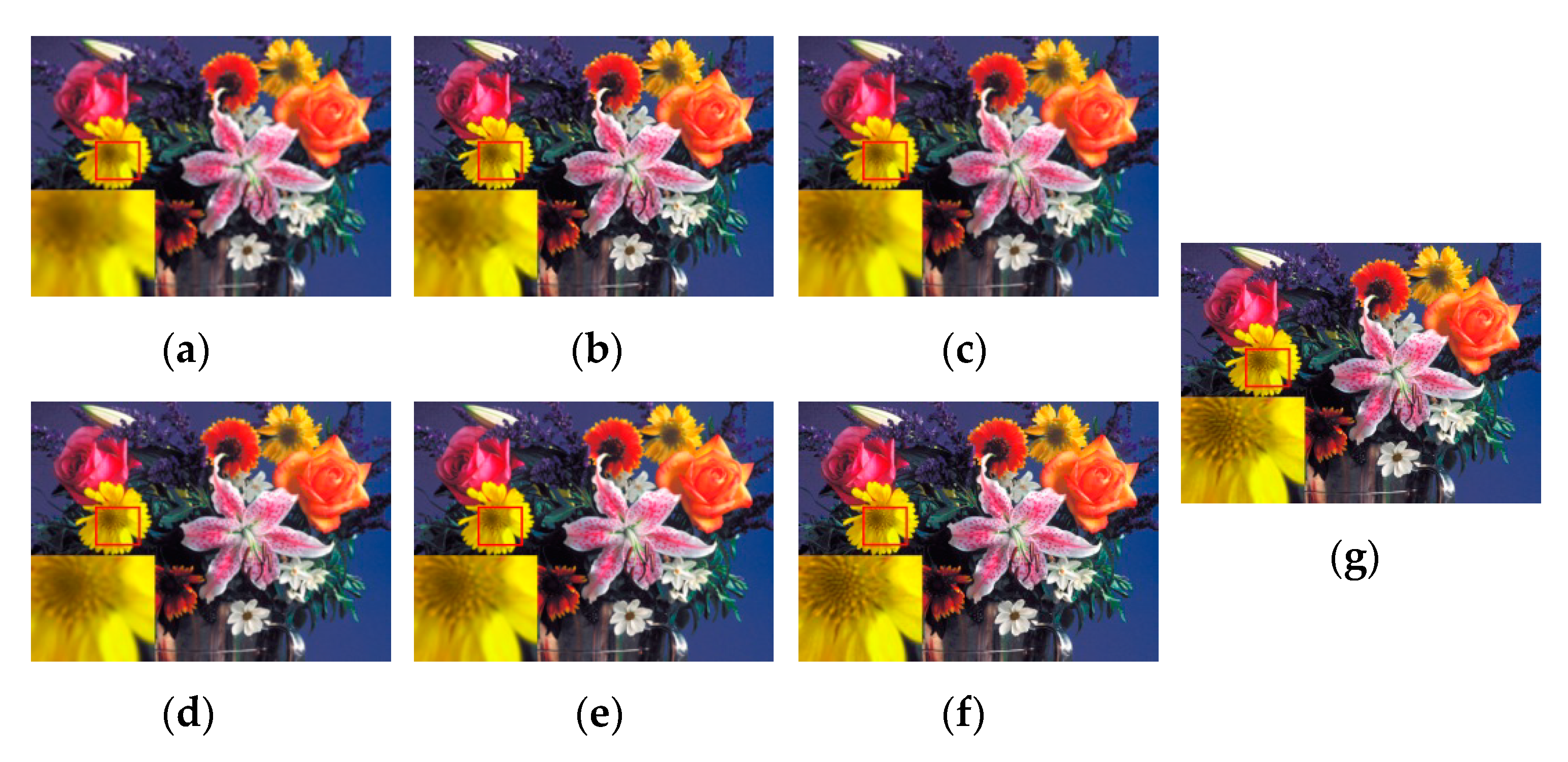
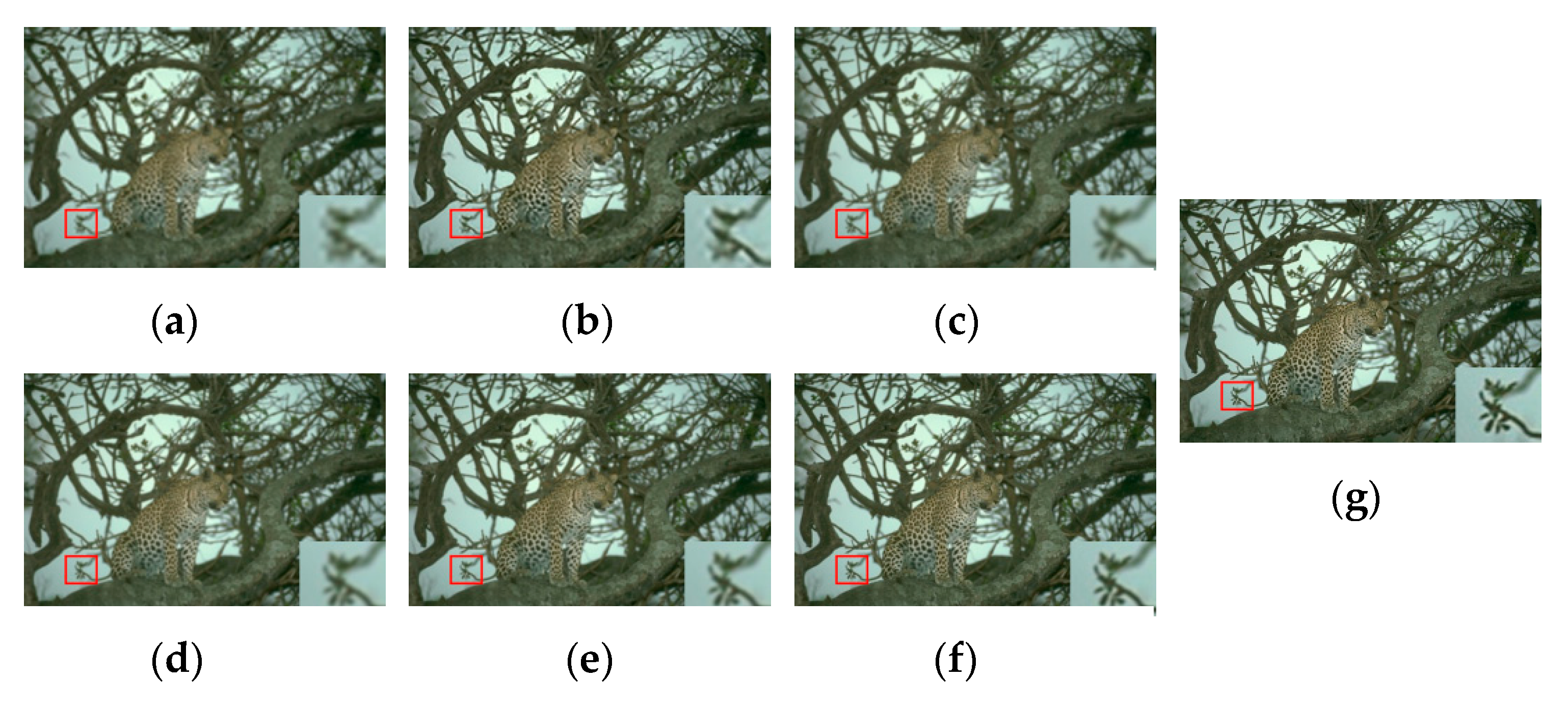
Then, we subjectively determined the quality of the output image and compared the performance of the six SR algorithms by observing the visual effects of the restored image. For comparison, given a 3× upscale factor, the restoration effects of the different SR algorithms used on the Set5, Set14, BSD100, and Urban100 test sets are shown in Figure 5, Figure 6, Figure 7 and Figure 8.
It can be intuitively seen from the figure that the reconstructed images of both traditional Bicubic and SRCNN have aliasing, while the restored image provided by our algorithm is clearer and sharper, and the reconstruction quality is better. In the details, as seen in the baby eye in Figure 5, petal color in Figure 6, branch texture in Figure 7, and building glass in Figure 8, MGEP-SRCNN reconstructed images have clearer features, have no sawtooth texture, and are more in line with the visual needs of the human eye.
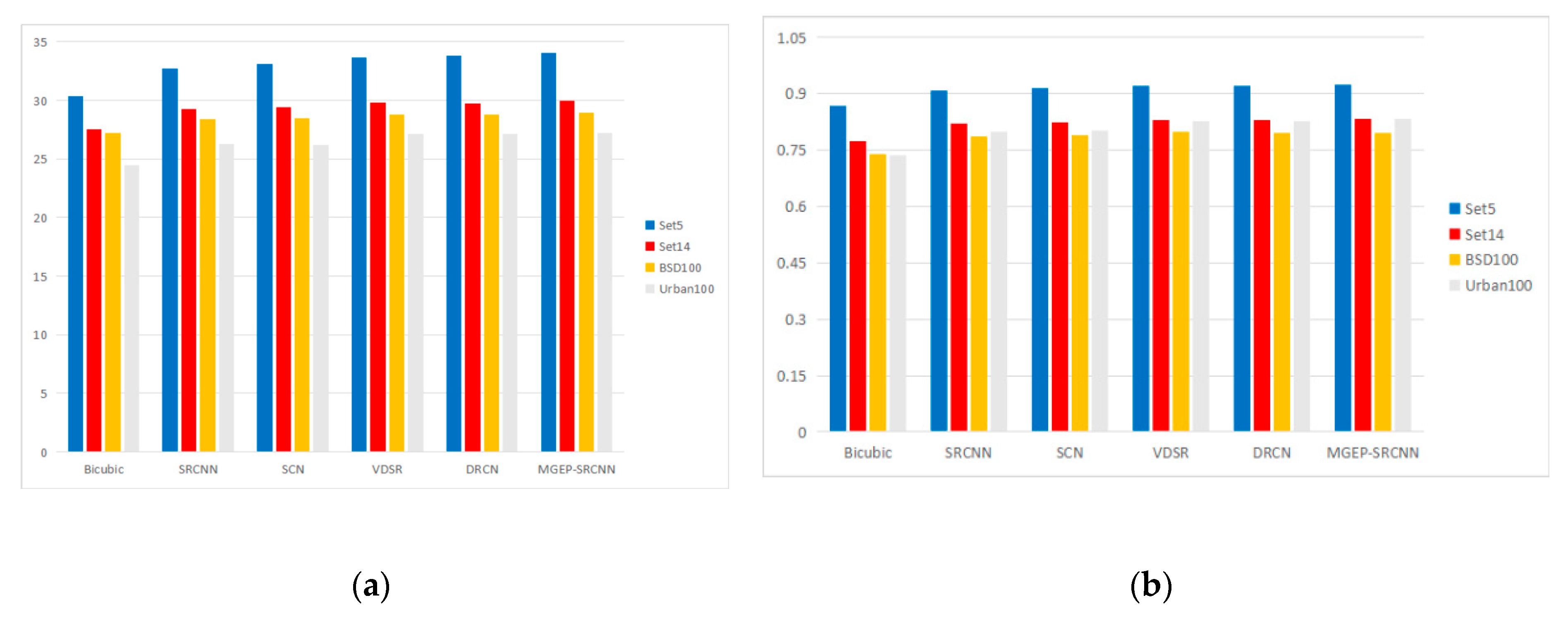
Figure 9 shows the PSNR/SSIM values of the six algorithms on the Set5, Set14, BSD100, and Urban100 test sets when the upscale factor was 3. The MGEP-SRCNN algorithm achieved the best PSNR effects in all four datasets. Except for the suboptimal data obtained in BSD100, the SSIM indicators were all optimal.

5. Conclusions

In this work, we presented a super-resolution method using Multilabel Gene Expression Programming. This method uses MGEP to extract a subset of image samples related to color and texture features in advance, and then performs nonlinear mapping and image reconstruction, thereby reducing the complexity of the convolutional neural network parameters so as to avoid the SR problems of slow training convergence and unstable recovery results. It was experimentally verified that the image restoration effect of this method under different magnifications and on training sets is better than that of the commonly used deep learning algorithms, and it also performs well in terms of subjective visual effects.

Author Contributions

Conceptualization, J.T.; methodology, C.H.; software, J.L.; validation, H.Z.; formal analysis, J.T.; investigation, C.H.; resources, J.L.; data curation, J.L.; writing—original draft preparation, J.T.; writing—review and editing, H.Z.; supervision, C.H.; funding acquisition, J.T. and H.Z. All authors have read and agreed to the published version of the manuscript.

Funding

This work was supported by the National Natural Science Foundation of China (61806088), by the Opening Project of Jiangsu Key Laboratory of Advanced Numerical Control Technology (SYKJ201804), by the Project funded by Jiangsu Province Postdoctoral Science Foundation (2019K041), and by Changzhou Sci&Tech Program (CE20195030).

Acknowledgments

We are grateful to our anonymous referees for their useful comments and suggestions. The authors also thank Honghui Fan, Yijun Liu, Yan Wang, Wei Gao and Jie Zhang for their useful advice during this work.

Conflicts of Interest

The authors declare no conflict of interest.

References

  1. Freeman, W.T.; Pasztor, E.C.; Carmichael, O.T. Learning Low-Level Vision. Int. J. Comput. Vision 2000, 40, 25–47. [Google Scholar] [CrossRef]
  2. Glasner, D.; Bagon, S.; Irani, M. Super-resolution from a single image. In Proceedings of the 2009 IEEE 12th International Conference on Computer Vision, Kyoto, Japan, 29 September–2 October 2009; pp. 349–356. [Google Scholar]
  3. Zhang, X.L.; Lam, K.M.; Shen, L.S. Image magnification based on a blockwise adaptive Markov random field model. Image Vis. Comput. 2008, 26, 1277–1284. [Google Scholar] [CrossRef]
  4. Freeman, W.T.; Jones, T.R.; Pasztor, E.C. Example-based super-resolution. IEEE Comput. Graph. Appl. 2002, 22, 56–65. [Google Scholar] [CrossRef] [Green Version]
  5. Dong, C.; Loy, C.C.; He, K.M.; Tang, X.O. Image Super-Resolution Using Deep Convolutional Networks. IEEE Trans. Pattern Anal. Mach. Intell. 2016, 38, 295–307. [Google Scholar] [CrossRef] [PubMed] [Green Version]
  6. Dong, C.; Loy, C.C.; Tang, X. Accelerating the Super-Resolution Convolutional Neural Network. In Proceedings of the Computer Vision—ECCV 2016; Springer: Cham, Switzerland, 2016; pp. 391–407. [Google Scholar]
  7. Hong, P.; Zhang, G. A Review of Super-Resolution Imaging through Optical High-Order Interference. Appl. Sci. 2019, 9, 1166. [Google Scholar] [CrossRef] [Green Version]
  8. Kim, J.; Lee, J.K.; Lee, K.M. Accurate image super-resolution using very deep convolutional networks. In Proceedings of the 2016 IEEE Conference on Computer Vision and Pattern Recognition, Las Vegas, NV, USA, 27–30 June 2016; pp. 1646–1654. [Google Scholar]
  9. Wang, Z.; Liu, D.; Yang, J.; Han, W.; Huang, T. Deep Networks for Image Super-Resolution with Sparse Prior. In Proceedings of the IEEE International Conference on Computer Vision, Santiago, Chile, 7–13 December 2015; pp. 370–378. [Google Scholar]
  10. Kim, J.; Lee, J.K.; Lee, K.M. Deeply-recursive convolutional network for image super-resolution. In Proceedings of the 2016 IEEE Conference on Computer Vision and Pattern Recognition, Las Vegas, NV, USA, 27–30 June 2016; pp. 1637–1645. [Google Scholar]
  11. Zhang, K.; Zuo, W.; Chen, Y.; Meng, D.; Zhang, L. Beyond a Gaussian Denoiser: Residual Learning of Deep CNN for Image Denoising. IEEE Trans. Image Process. 2017, 26, 3142–3155. [Google Scholar] [CrossRef] [PubMed] [Green Version]
  12. Zhang, K.; Zuo, W.; Gu, S.; Zhang, L. Learning deep CNN denoiser prior for image restoration. In Proceedings of the IEEE Conference on Computer Vision and Pattern Recognition, Honolulu, HI, USA, 21–26 July 2017; pp. 3929–3938. [Google Scholar]
  13. Lim, B.; Son, S.; Kim, H.; Nah, S.; Lee, K.M. Enhanced deep residual networks for single image super-resolution. In Proceedings of the IEEE Conference on Computer Vision and Pattern Recognition Workshops, Honolulu, HI, USA, 21–26 July 2017; pp. 136–144. [Google Scholar]
  14. Hayat, K. Multimedia super-resolution via deep learning: A survey. Digit. Signal Process. 2018, 81, 198–217. [Google Scholar] [CrossRef] [Green Version]
  15. Yang, W.; Zhang, X.; Tian, Y.; Wang, W.; Xue, J.; Liao, Q. Deep Learning for Single Image Super-Resolution: A Brief Review. IEEE Trans. Multimedia 2019, 21, 3106–3121. [Google Scholar] [CrossRef] [Green Version]
  16. Zhang, H.J.; Gong, Y.H.; Low, C.Y.; Smoliar, S.W. Image retrieval based on color features: An evaluation study. In Proceedings of the SPIE, Digital Image Storage and Archiving Systems, Philadelphia, PA, USA, 21 November 1995; pp. 212–220. [Google Scholar]
  17. Haralick, R.M.; Shanmugam, K.; Dinstein, I. Textural Features for Image Classification. IEEE Trans. Syst. Man. Cybern. 1973, SMC-3, 610–621. [Google Scholar] [CrossRef] [Green Version]
  18. Ferreira, C. Gene Expression Programming: A New Adaptive Algorithm for Solving Problems. Complex Syst. 2001, 13, 87–129. [Google Scholar]
  19. Zhou, C.; Xiao, W.M.; Tirpak, T.M.; Nelson, P.C. Evolving accurate and compact classification rules with gene expression programming. IEEE Trans. Evol. Comput. 2003, 7, 519–531. [Google Scholar] [CrossRef] [Green Version]
  20. Choi, J.; Kim, M. Single Image Super-Resolution Using Global Regression Based on Multiple Local Linear Mappings. IEEE Trans. Image Process. 2017, 26, 1300–1314. [Google Scholar] [CrossRef] [PubMed]
  21. Bevilacqua, M.; Roumy, A.; Guillemot, C.; Morel, M.L.A. Low-Complexity Single-Image Super-Resolution based on Nonnegative Neighbor Embedding. In Proceedings of the British Machine Vision Conference (BMVC), Guildford, Surrey, UK, 3–7 September 2012; pp. 1–10. [Google Scholar]
  22. Zeyde, R.; Elad, M.; Protter, M. On Single Image Scale-Up Using Sparse-Representations. In Proceedings of the International Conference on Curves and Surfaces; Springer: Berlin/Heidelberg, Germany, 2012; pp. 711–730. [Google Scholar]
  23. Martin, D.; Fowlkes, C.; Tal, D.; Malik, J. A database of human segmented natural images and its application to evaluating segmentation algorithms and measuring ecological statistics. In Proceedings of the Eighth IEEE International Conference on Computer Vision (ICCV), Vancouver, BC, Canada, 7–14 July 2001; pp. 416–423. [Google Scholar]
  24. Huang, J.B.; Singh, A.; Ahuja, N. Single image super-resolution from transformed self-exemplars. In Proceedings of the IEEE Conference on Computer Vision and Pattern Recognition (CVPR), Boston, MA, USA, 7–12 June 2015; pp. 5197–5206. [Google Scholar]
  25. He, K.; Zhang, X.; Ren, S.; Sun, J. Delving Deep into Rectifiers: Surpassing Human-Level Performance on ImageNet Classification. In Proceedings of the 2015 IEEE International Conference on Computer Vision (ICCV), Santiago, Chile, 7–13 December 2015; pp. 1026–1034. [Google Scholar]
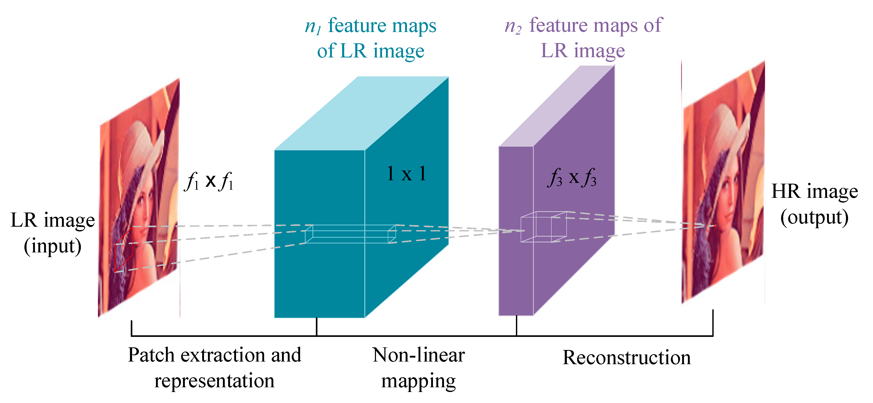
Figure 1. Network architecture of the super-resolution convolution neural network (SRCNN).
Applsci 10 00854 g001
Figure 2. Color histogram of an image (RGB channel).
Applsci 10 00854 g002
Figure 3. The Multilabel Gene Expression Programming (MGEP) preclassification model.
Applsci 10 00854 g003
Figure 4. MGEP-SRCNN algorithm flow chart.
Applsci 10 00854 g004
Figure 5. Super-resolution restoration results of the image “Baby” in Set5 [21]. (a) Bicubic; (b) SRCNN [5]; (c) SCN [9]; (d) VDSR [8]; (e) DRCN [10]; (f) MGEP-SRCNN; (g) Ground truth.
Applsci 10 00854 g005
Figure 6. Super-resolution restoration results of the image “Flowers” in Set14 [22]. (a) Bicubic; (b) SRCNN [5]; (c) SCN [9]; (d) VDSR [8]; (e) DRCN [10]; (f) MGEP-SRCNN; (g) Ground truth.
Applsci 10 00854 g006
Figure 7. Super-resolution restoration results of the image “016” in BSD100 [23]. (a) Bicubic; (b) SRCNN [5]; (c) SCN [9]; (d) VDSR [8]; (e) DRCN [10]; (f) MGEP-SRCNN; (g) Ground truth.
Applsci 10 00854 g007
Figure 8. Super-resolution restoration results of the image “002” in Urban100 [24]. (a) Bicubic; (b) SRCNN [5]; (c) SCN [9]; (d) VDSR [8]; (e) DRCN [10]; (f) MGEP-SRCNN; (g) Ground truth.
Applsci 10 00854 g008
Figure 9. Image restoration results of the six SR algorithms. (a) PSNR; (b) SSIM.
Applsci 10 00854 g009
Table 1. Average Peak Signal-to-Noise Ratio (PSNR)/Structural Similarity (SSIM) values for 2× scale. Red color indicates the best and the blue color indicates the second-best performance.
DatasetBicubicSRCNN [5]SCN [9]VDSR [8]DRCN [10]MGEP-SRCNN
Set533.66/0.929936.66/0.954236.93/0.955237.53/0.958737.63/0.958837.78/0.9594
Set1430.24/0.868832.42/0.906332.56/0.907433.03/0.912433.04/0.911833.29/0.9135
BSD10029.56/0.843131.36/0.887931.40/0.888431.90/0.896031.85/0.894232.01/0.8979
Urban10026.88/0.840329.50/0.894629.50/0.896030.76/0.914030.75/0.913331.19/0.9181
Table 2. Average PSNR/SSIM values for 3× scale. Red color indicates the best and the blue color indicates the second-best performance.
DatasetBicubicSRCNN [5]SCN [9]VDSR [8]DRCN [10]MGEP-SRCNN
Set530.39/0.868232.75/0.909033.10/0.914433.66/0.921333.82/0.922634.04/0.9250
Set1427.55/0.774229.28/0.820929.41/0.823829.77/0.831429.76/0.831129.97/0.8333
BSD10027.21/0.738528.41/0.786328.50/0.788528.82/0.797628.80/0.796328.92/0.7972
Urban10024.46/0.734926.24/0.798926.21/0.801027.14/0.827927.15/0.827627.24/0.8330
Table 3. Average PSNR/SSIM values for 4× scale. Red color indicates the best and the blue color indicates the second-best performance.
DatasetBicubicSRCNN [5]SCN [9]VDSR [8]DRCN [10]MGEP-SRCNN
Set528.42/0.810430.48/0.862830.86/0.873231.35/0.883831.53/0.885431.66/0.8899
Set1426.00/0.702727.49/0.750327.64/0.757828.01/0.767428.02/0.767028.19/0.8359
BSD10025.96/0.667526.90/0.710127.03/0.716127.29/0.725127.23/0.723327.34/0.7238
Urban10023.14/0.657724.52/0.722124.52/0.725025.18/0.752425.14/0.751025.21/0.7837
Table 4. Comparison of the running times (sec) for scales 2×, 3×, and 4×. Red color indicates the best performance.
DatasetScaleBicubicSRCNN [5]SCN [9]VDSR [8]DRCN [10]MGEP-SRCNN
Set5×2-2.1910.9410.0540.7350.039
×3-2.2351.8290.0620.7480.052
×4-2.1931.2450.0540.7350.044
Set14×2-4.3241.7090.1131.5790.097
×3-4.4023.6110.1221.5690.113
×4-4.3972.3770.1121.5260.101
BSD100×2-2.5171.0150.0710.9830.069
×3-2.5832.1380.0710.9960.067
×4-2.5161.2900.0710.9840.061
Urban100×2-22.1234.7790.4515.0100.401
×3-19.3584.0120.5145.0540.484
×4-18.4623.1990.4485.0480.407