1. Introduction
Variable-speed wind turbines (VSWTs) have been dominating the wind power market for decades, resulting in the emergence of effective strategies to improve its power coefficient (
Cp). Maintaining the optimal tip speed ratio (TSR) by adjusting the rotor speed dynamically will contribute to maximum
Cp in the variable speed region. The strategies to maintain
Cp or power close to its maximum value (TSR to optimal TSR) is known as maximum power point tracking (MPPT). There are four main categories of the MPPT methods: power signal feedback (PSF) control, perturbation and observation (P&O) control, tip-speed ratio (TSR) control, and optimal torque (OT) control [
1,
2,
3]. PSF control and OT control are similar in performance and commonly used in large-scale wind turbines [
4]. This paper focuses on the OT control method.
The conventional OT control method has a good performance in small-scale wind turbines since the dynamic response of small-scale wind turbines is swift enough. Regardless of the dynamic transient behavior of VSWTs, the conventional OT control method is based on the steady optimal generator torque versus the generator speed curve. However, there is no absolute steady-state for VSWTs due to the stochastic nature of the wind speed under real conditions. Unfortunately, the increasing tendency in size and capacity of VSWTs will aggravate the conflict between the rapid wind variations (especially for the wind conditions with a low average value and high turbulent density) and the slow dynamic response of wind turbines owing to the large inertia of the rotor and generator. Previous research [
5,
6,
7,
8,
9] has demonstrated that the slow dynamic response resulting from large inertia of VSWTs leads to the power loss of MPPT. The frequency of the wind speed variations and the average value of wind speed also play a great role in power loss [
6,
7,
8]. Therefore, it is vital and valuable to find a novel MPPT method to enable large-scale VSWTs to respond better to the rapid wind variations.
Huang et al. [
10] focused on the short-term maximum energy optimization instead of the instantaneous maximum power capture. They used semi-definite programming (SDP) to execute the optimal reference command in an intelligent way considering the short-term wind speed prediction, maximum short-term energy, and wind turbine dynamic response collectively. Nevertheless, the time period for the short-term maximum energy optimization hasn’t been adjusted corresponding to the nonlinear dynamics of VSWTs. Some system correction methods, including the differential control based on rotor speed and feed-forward control based on aerodynamic torque and generator torque, have been applied to MPPT control by previous researchers [
11,
12,
13]. However, previous research [
11,
12,
13] didn’t figure out the method to design the proportional gain in the correction path. Zhou et al. [
14] reduced the MPPT tracking range considering the dynamic wind performance (mean wind speed, turbulence intensity, and turbulence frequency), which improved the ability of MPPT to track varying turbulent wind at the expense of power loss under low-speed wind conditions. Mao et al. [
15] proposed an adaptive robust control (ARC) method to overcome the power reduction resulting from uncertain factors, including wind variations. Zhao et al. [
16] found that regulating the blade-pitch angle dynamically within a slight range, according to instantaneous TSR could increase the power by 0.2% to 3.4% in the MPPT region. However, Zhao et al. didn’t provide the method to estimate TSR. Yin et al. [
17,
18] proposed a multi-point method for aerodynamic optimization of VSWT blades considering the distribution of operational TSR and an inverse aerodynamic optimization to focus on determining an appropriate design TSR. The aerodynamic optimization focusing on blade remolding may cost a lot of money.
Considering the nonlinear and slow dynamics of VSWTs, the feed-forward control is added to the conventional OT control method, and the collective blade-pitch angle is regulated dynamically according to instantaneous TSR. Aerodynamic torque is estimated using the unscented Kalman filter (UKF). Wind speed and TSR are estimated using the Newton–Raphson method. The error between the estimated aerodynamic torque and the optimal steady torque is used as the feed-forward signal to control generator torque. Gain parameters in the feed-forward path are nonlinearly regulated by the estimated generator speed. Meanwhile, the estimated TSR is used as the reference signal for the optimal blade-pitch angle regulation under non-optimal TSR conditions, which can improve the wind power capture under a wider non-optimal TSR range. The example of a 5 MW wind turbine model is presented and analyzed.
2. Model of Wind Turbine Systems
Modeling of the electromagnetic dynamics of the doubly-fed induction generator (DFIG) system is based on assumptions 1–3:
All of the stator and rotor quantities are transformed into a stationary frame (the d-q frame) using the Park transformation in terms of the stator’s and rotor’s voltage-pulsation frequencies ωs and ωr, respectively. In addition, the Park transformation is based on an equivalent power principle.
The stator flux is constant. The q-axis is aligned with the stator flux vector. The d-axis is aligned with the stator voltage vector.
The stator’s resistive voltage drop is neglected.
Modeling of the wind turbine dynamic drive-train is based on assumptions 4–5:
- 4.
The rotor speed, the equivalent rotor speed, and the generator speed are always positive when wind turbines work normally. The aerodynamic torque is positive towards the accelerating direction of the drive-train. The electromagnetic torque is positive towards the decelerating direction of the drive-train.
- 5.
The moment of inertia of the drive-train shafts and the gearbox is neglected.
2.1. Electromagnetic Dynamics of the DFIG System
The electromagnetic dynamics of the DFIG system is described in this section. The mechanical dynamics of the DFIG system will be described in the next section since the shaft of the DFIG system is coupled to the drive-train. The DFIG system is nonlinear and mutually coupled between the stator phases and rotor phases. As described in assumption 1, the Park transformation is applied to decouple the stator phases and rotor phases. In the d-q frame, the dynamic equation of the DFIG system with constant coefficients is [
19,
20]:
where
u,
i,
ψ,
R, and
ω represent voltage, current, flux, resistance, rotational speed, respectively; subscripts r, s, d, q represent rotor-side, stator-side, d-axis, and q-axis, respectively. Note that
ωs is synchronous speed, and
ωg is the mechanical speed of the generator rotor. d/dt represents the differential operator.
In the d-q frame, the flux equation of the DIFG system is [
19,
20]:
where
Ls,
Lr, and
Lm represent the self-inductance of the equivalent stator winding, the self-inductance of the equivalent rotor winding, and mutual inductance between the equivalent stator winding and the equivalent rotor winding, respectively.
The electromagnetic torque of the DIFG system is [
19,
20]:
where
np represents the number of pole pairs.
Under assumption 2, the stator flux and voltage in d-q frame are:
where
Us is the stator voltage.
Substituting Equation (2) into Equation (4) produces the relationships between the equivalent rotor currents and the equivalent stator currents:
Under assumptions 1–3, the dynamic equation of the DFIG system is:
where:
Under assumptions 1–3, substituting Equations (4) and (5) into Equation (3) produces:
2.2. Dynamic Drive-Train
The dynamics of the wind turbine drive-train can be modeled as the two-mass model by making the rotor of wind turbines and the gearbox equivalent to one-mass model on the side of the high-speed shaft, as shown in
Figure 1. In this model,
n is the gearbox ratio;
is the moment inertia of rotor and
is the equivalent value;
is the moment inertia of generator;
is the aerodynamic torque of wind turbines and
is the equivalent aerodynamic torque;
is the rotor speed of wind turbines and
is the equivalent value;
and
represent the equivalent damping and stiffness of the two-mass model, respectively.
The damping torque is mainly generated by the friction and is proportional to rotor speed. The stiffness torque is mainly generated by the torsion of the drive-train shafts and is proportional to the torsional angle of equivalent shafts. Under assumptions 4–5, the dynamics of the wind turbine drive-train is:
where
is the equivalent rotor angular displacement.
is the generator angular displacement.
The mechanical dynamics of the DFIG system is analyzed in the dynamics of the wind turbine drive-train since the shaft of the DFIG system is coupled to the drive-train, as shown in the third formula of Equation (9). The state-space form of Equation (9) is:
where:
The aerodynamic power extracted from the wind is:
where
ρ is the air density;
R is the rotor radius;
v is the wind speed;
Cp is the power coefficient;
β is the collective blade-pitch angle;
λ is the TSR;
Cp(
λ,
β) is used to show the value of
Cp mainly depends on
λ and
β.The aerodynamic torque is:
where:
3. Wind Turbine Inertial Response Time
The response time of using electronic components to control current and electromagnetic torque is far less than that of wind turbine drive-train dynamics. Both the moment of inertia and the wind variations are the main factors leading to the power loss of MPPT. The wind turbine inertial response time τ is defined as the time interval between two steady-state speeds when the shaft speed reaches to 63.2% of the total change, which reveals the effect of wind turbine inertia on power loss of MPPT. The inertial response time τ is able to be obtained by the numerical method and analytical method. The numerical method refers to perturbing the wind speed at each operating point and measuring the resulting variations in the generator speed. The analytical method refers to using mathematics to obtain the theoretical formula of τ. The analytical method is based on assumptions 6–8:
- 6.
The response time of realizing the expected electromagnetic torque is neglected.
- 7.
The equivalent stiffness is infinite.
- 8.
The equivalent damping is far less than .
Under assumption 7, the equivalent rotor speed will be synchronous with the generator speed:
Under assumption 6–8, substituting Equation (18) into Equation (9) produces:
In the conventional MPPT method, the optimal steady electromagnetic torque is [
11]:
where
is the maximum power coefficient;
is the optimal TSR.
Equation (22) can be written as:
Linearized model of Equation (22) can be obtained using the Taylor expansion [
21]:
where
and
is the total differential symbol and the partial differential symbol, respectively.
Under assumptions 6–8, taking the Laplace transform of Equation (24) produces a first-order model at the working point (
):
where:
where
Kg is also the partial of
ωg with respect to
v.
When the wind turbine works at the optimal working point, we can obtain:
Substituting Equations (22) and (28) into Equations (26) and (27) produces:
From the analytical result,
Kg is constant, and
τ is inversely proportional to the generator speed. The numerical method perturbing the wind speed at each operating point is also carried out to obtain the value of
τ. The numerical and analytical results of the inertial response time are shown in
Figure 2. The numerical results are very close to the analytical ones. The few differences among them may result from the fact that the numerical results are based on the relatively real conditions, while the analytical results are based on assumptions 6–8.
For the first-order model, the cutoff frequency is the reciprocal of the time constant. The tracking bandwidth of the first-order model,
, which also reflects the wind turbine response performance to wind variations, refers to the frequency width from zero to the cutoff frequency. The wider
is, the faster dynamic response wind turbines show. Hence, the tracking bandwidth of the first-order model is equal to the reciprocal of
τ:
The results above demonstrate that wind turbines show a relatively poor tracking performance under conditions with low generator speed (or wind speed) while using the conventional MPPT method.
4. Deficiencies of the Conventional MPPT Method from Other Perspectives
Apart from the narrow tracking bandwidth and slow dynamic response under conditions with low wind speed, the conventional MPPT method shows its deficiencies because of the following two assumptions.
4.1. Neglecting the Variations of Kinetic Energy Stored in the Rotor and Generator
Apart from the mechanical transmission loss and the electromagnetic loss, rotating parts will absorb or release kinetic energy while converting wind energy into electric energy. The power flow of the wind energy generation systems is:
where,
represents the mechanical transmission power loss and the electromagnetic power loss;
represents the electric power;
represents the derivative of kinetic energy stored in rotor and generator.
Figure 3 describes the power flow of the wind energy generation system. The rotating parts (rotor, generator, gearbox, and so forth) in VSWTs serve as energy storage devices that extract energy from the wind while accelerating and release kinetic energy to the grid while decelerating. As the growing moment of inertia of rotating parts, the speed for rotating parts to extract and release energy will slow down, which means slower dynamic response to wind variations. Actually, the goal of MPPT control is to regulate the instantaneous aerodynamic power instead of the instantaneous electric power to the optimal value. Conventional OT and PSF method set instantaneous electric power to optimal value and neglect the variations of kinetic energy stored in rotating parts assuming the VSWTs’ response to wind variations is fast enough. However, response time is needed for the dynamic process of instantaneous aerodynamic power (or torque) to reach the setting instantaneous electric power (or torque). There exists significant power loss in that process. It is valuable to find a novel wind turbine MPPT method to shorten the dynamic process for instantaneous aerodynamic power (or torque) to reach the set value.
4.2. Assumption of the Optimal TSR All the Time
As mentioned above, there is no absolutely steady-state for VSWTs because of the stochastic nature of wind. TSR will fluctuate around the optimal TSR rather than maintain the absolute optimal TSR all the time. The conventional OT method operates under a fixed collective blade-pitch angle corresponding to the optimal TSR. However, the optimal collective blade-pitch angle varies with the instantaneous TSR.
Cp, as a function of TSR and the collective blade-pitch angle, is calculated using the AeroDyn standalone code. The contour map of
Cp(
λ,
β) of a 5 MW wind turbine is shown in
Figure 4.
5. Design of the Improved MPPT Control Method
The design of the improved MPPT control method is based on assumptions 9–10:
- 9.
The equivalent aerodynamic torque remains unchanged during one discrete time step while discretizing Equation (10).
- 10.
The blade-pitch actuator dynamic effects can be simulated by the first-order model with a time constant of 3 s.
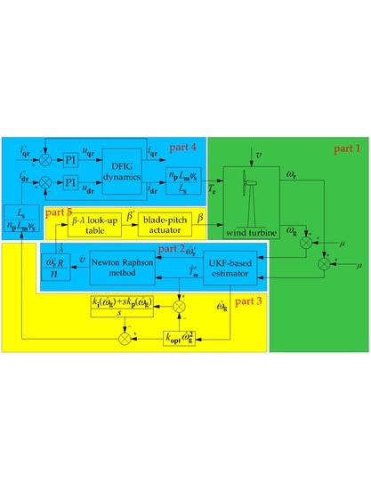
Figure 5 shows the control diagram of the improved MPPT control method considering the wind turbine dynamic response. There are five parts marked in three colors. The aerodynamics and mechanical aspects of wind turbines are established using the FAST code in part 1. Part 2–5 are realized in MATLAB/SIMULINK (MathWorks, Natick, MA, USA). FAST (National Renewable Energy Laboratory, Golden, CO, USA) interfaces with MATLAB/SIMULINK using S-function. In part 2, aerodynamic torque is estimated using the UKF-based estimator. Wind speed and TSR are estimated using the Newton–Raphson method. In part 3, the feed-forward control is used to improve the dynamic response of wind turbines. The error between the estimated aerodynamic torque and the optimal steady torque is used as the feed-forward signal to control generator torque. To get better performance under various wind conditions, gain parameters in the feed-forward path are nonlinearly regulated by the estimated generator speed. In part 4, a DFIG model is built in MATLAB/SIMULINK for simulating the dynamic process of the DFIG system and achieving the setting value of the electromagnetic torque. Meanwhile, the estimated TSR is used as the reference signal for the optimal collective blade-pitch angle regulation under non-optimal TSR conditions in part 5, which can improve the wind power capture under a wider non-optimal TSR range.
5.1. Estimation of Equivalent Aerodynamic Torque
As shown in Equation (10), the observable states,
and
, can be used to estimate the equivalent aerodynamic torque
using the UKF-based estimator with clipping and uncorrelated conversion. The discretized state-space model is necessary for estimating variables. Under assumption 9, the discretized form of Equation (10) is:
where
and
represent the process noise vectors and measurement noise vectors, respectively; and the matrix
G and
H are:
where
Ts is the sampling step. The estimated values of the equivalent aerodynamic torque, the equivalent rotor speed, and the generator speed are written as
,
, and
, respectively.
5.2. Estimation of the Equivalent Wind Speed
The estimation of the equivalent wind speed is a process to solve the nonlinear Equation (34):
The Jacobian of function
is:
The Newton-Raphson method is utilized to solve Equation (34). The procedure is [
22]:
Initialize the wind speed .
Calculate the increment .
Calculate the wind speed in the next step , .
If , stop. Else get back to step 2. where is the threshold for estimation.
The instantaneous equivalent TSR is:
5.3. Feed-Forward Control with the PI Gain Scheduling
Previous research [
11,
12] has already focused on the error feed-forward control based on aerodynamic torque and generator torque. However, they didn’t figure out the method to design the proportional gain in the correction path. Meanwhile, the feed-forward control with the fixed gain certainly haa a good performsnce at a few working points due to the nonlinear dynamic performance of VSWTs under various wind conditions. The nonlinear problem has been solved in this paper. Gain scheduling control, feed-forward control, and the conventional OT control are combined to endow VSWTs with a good dynamic performance at most of the working points.
To get better performance under small wind variations or nearly steady wind conditions, the integral control is added to the feed-forward path. Thus the new electromagnetic torque setting value is:
where
,
represent the proportional and integral gain in the feed-forward path, respectively.
Under assumptions 6–8, using Taylor expansion mentioned in Equation (24) produces:
Substituting Equation (29) into Equation (38) produces:
where:
Amplitude-frequency characteristic of the system described by Equation (39) is:
Subsequently, the bandwidth
is:
where
is defined as the transfer coefficient from
to
.
The wind turbine nonlinear system is able to work as the second-order linear system does by regulating the gain
,
nonlinearly to maintain the bandwidth
and the damping ratio
to constant. The reference constant of
is supposed to be assigned considering the typical wind spectrum and the capacity of wind turbines.
is assigned to 0.6 rad s
−1 for a 5 MW wind turbine model [
23]. The damping ratio
is assigned to 0.707. The gains
,
are:
The regulating shame can is also shown in
Figure 6.
When wind turbines start or large wind variations occur, the integral value in the feed-forward path will accumulate, which may result in high overshoot and system oscillations. Integral separation Algorithm 1 is adopted to solve that problem. Here list the rules of integral separation Algorithm 1:
| Algorithm 1 |
If : the integral part will be separated. If : the integral part will work. Rising edge command and descending edge command are applied to clear the data stored in the integrator when the controller begins to separate or introduce an integral part. where is the threshold for the integral separation algorithm.
|
5.4. Regulation of Optimal Collective Blade-Pitch Angle
As shown in
Figure 4, the optimal collective blade-pitch angle varies with the instantaneous TSR. Interpolation function is used to establish the lookup table between the optimal collective blade-pitch angle and the instantaneous TSR based on the results from AeroDyn:
where lookup represents one-dimensional interpolation function with the instantaneous TSR serving as input and the optimal setting value of the collective blade-pitch angle serving as output.
The collective blade-pitch angle is saturated to a maximum of 2°, and a minimum of −2° in the MPPT region since too wide blade-pitch angle regulation may cost too much energy from the variable-pitch system and bring in more extra fatigue loads to VSWTs.
Under assumption 10, the mathematical model of the blade-pitch actuator is:
6. Performance Validation
The performance validation is based on assumptions 11:
- 11.
The pitch angle is fixed at β = −1.0° in the conventional OT method.
FAST code is used to simulate the aerodynamics and the mechanical aspects of wind turbines, while MATLAB/SIMULINK is used to simulate the DFIG system. This section compares the simulation results of a 5 MW wind turbine using the novel MPPT method with that using the conventional OT method. The parameters used are shown in
Table 1.
The Cp(λ, β) of the 5 MW wind turbine calculated by AeroDyn shows the Cpmax equals 0.4648 when λ = λopt = 7.057 and β = βopt = −1.0°. Thus, the pitch angle is fixed at β = −1.0° in the conventional OT method corresponding to assumption 11.
To avoid short-term overloading of the generator and the gearbox, the electromagnetic torque is saturated to a maximum of 47,402.91 N·m, and a torque rate limit of 15,000 N·m·s
−1 is also imposed [
23].
6.1. Dynamic Response of Step Wind
In order to test the dynamic response between two steady states, wind speed profiles with a unit step at 5 m/s, 7 m/s, and 9 m/s are used, as shown in
Figure 7a.
Figure 7b depicts the blade-pitch angle. During the periods of stable wind conditions, there is only a little difference (less than 0.2°) of the blade-pitch angle at 5 m/s, 7 m/s, and 9 m/s. That phenomenon may result from the relatively imprecise calculation of the optimal blade-pitch angle. During the dynamic periods, the blade-pitch angle varies from −1.41° to −0.74° at 5 m/s, from −1.28° to −0.81° at 7 m/s and from −1.13° to −0.87° at 9 m/s. As analyzed in
Section 3, the dynamic response of VSWTs tends to be slower, and TSR tends to vary in the wider range under lower-speed wind conditions, which can account for wider variations in the blade-pitch angle at 5 m/s.
Figure 7c demonstrates the dynamic response of rotor speed. Obviously, during periods of stable wind conditions, there is no difference between the conventional method and the novel method. It takes about 30 s, 20 s, and 15 s for the transition process between two steady states at 5 m/s, 7 m/s, and 9 m/s, respectively, while using the conventional OT method. This result corresponds to the nonlinear performance as mentioned in
Section 3. While using the novel MPPT method proposed in the paper, it only takes about 6 s for VSWTs to achieve the other steady-state, whatever at 5 m/s, 7 m/s, or 9 m/s. Thus, the novel MPPT method has assuredly shortened the dynamic transition process between two steady states.
Figure 7d depicts the cumulative electric energy increment between using the novel MPPT method and using the conventional MPPT method. With the increasing unit step in wind velocity, higher wind energy is stored in rotating parts as the kinetic energy to accelerate the rotor speed by the novel method than that by the conventional OT method during the period of [100 s–105 s]. Hence, the electric energy output is first less, and then becomes more as the kinetic energy is released to the grid during the period of [105 s–140 s]. With the decreasing unit step in wind velocity, the kinetic energy releases faster to decelerate the rotor speed during the period of [140 s–d145 s]. Correspondingly, during the period of [60 s–180 s], the cumulative electric energy increment has significantly increased by 0.068 kw·h, 0.044 kw·h, and 0.028 kw·hat 5 m/s, 7 m/s, and 9 m/s, respectively. Therefore, the novel MPPT method shows more remarkable effects in the dynamic response of the rotor speed and the cumulative electric energy extraction than the conventional MPPT method, especially under lower-speed wind conditions.
6.2. Dynamic Response of Sinusoidal Wind Containing Several Frequencies
In order to test the bandwidth of the conventional MPPT method and the novel MPPT method, a sinusoidal wind profile containing several frequencies is used for simulation, as shown in
Figure 8a. The wind profile is defined by:
From
Figure 3, the rotating parts of wind turbines absorb or release kinetic energy while converting wind energy into electric energy. The mechanical energy extracted from the inflow wind can’t be accurately measured. The electric energy or the electric power is usually used to represent the wind turbine power performance. However, the change in kinetic energy stored in rotating parts will disturb the results if we use electric energy to represent the energy extracted from the wind. To solve that problem, kinetic energy stored in rotating parts is expected to maintain the same at the beginning and the end of the analysis period. Correspondingly, the wind speed in the period of [0 s–50 s] and [200 s–250 s] will be both set as the constant, 8 m/s. The analysis period is [50 s 200 s]. The black line and red line represent the simulating wind and the estimated wind, respectively, in
Figure 8a. Notably, the UKF-based estimator and the Newton–Raphson method work well to estimate the turbulent wind speed with high accuracy.
Figure 8b depicts the blade-pitch angle. Obviously, while using the novel MPPT method, the blade-pitch angle varies around −1°, corresponding to the value of using the conventional MPPT method.
Figure 8c demonstrates the dynamic response of rotor speed. While using the conventional MPPT method, wind turbines show better performance in tracking the wind variations under high-speed wind conditions during the period of [50 s–100 s], and relatively worse performance under the low-speed wind conditions during the period of [130 s–180 s]. That affirms the nonlinear property of VSWTs while using the conventional MPPT method.
Figure 8d depicts the cumulative electric energy increment between using novel MPPT method and using the conventional MPPT method. Obviously, the electric energy extracted from wind has significantly increased by 0.59 kW·h from 50 s to 250 s. That affirms the energy improvement of the novel MPPT method.
Figure 8e shows the frequency spectrum of rotor speed corresponding to the time-domain graphics in
Figure 8c. From Equation (30), the bandwidth is supposed to vary from 0.05 rad/s to 0.2 rad/s while using the conventional MPPT method and is designed to maintain around 0.6 rad/s while using the novel MPPT method. Thus, both the conventional method and the novel method are able to track the wind components of the frequency, 0.05 rad/s, as shown in
Figure 8e. The amplitude response to the wind components of the frequencies, 0.2 rad/s, and 0.6 rad/s, shows that wind turbines significantly track the wind variations better using the novel MPPT method than that using the conventional MPPT method. That affirms the improved tracking bandwidth of the novel MPPT method.
6.3. Dynamic Response of the Typical Turbulent Wind
The turbulent wind profile contains wind components of various frequencies, which is suitable to simulate the real wind conditions. Therefore, a typical turbulent wind profile is used to test the wind turbine MPPT dynamic response under real wind conditions.
As described in
Section 6.2, the wind speed during periods of [0 s–50 s] and [200 s–250 s] are both set as the constant, 8 m/s. The analysis period is [50 s–200 s].
Figure 9a shows the turbulent wind profile and the estimated value. The black line and red line represent the simulating wind and the estimated wind, respectively. Notably, the UKF-based estimator and the Newton–Raphson method work well to estimate the turbulent wind speed with high accuracy.
Figure 9b depicts the blade-pitch angle. Obviously, the blade-pitch angle while using the novel MPPT method varies around −1°, corresponding to the value of using the conventional MPPT method.
Figure 9c shows the dynamic response of rotor speed. During the period of [50 s 200 s], wind turbine tries to track, but seriously lag behind the wind components of low frequencies while using the conventional MPPT method.
Figure 9d depicts the cumulative electric energy increment between using the novel MPPT method and using the conventional MPPT method. Obviously, the electric energy extracted from wind has significantly increased by 0.21 kW·h from 50 s to 250 s. That affirms the energy improvement of the novel MPPT method. Besides, wind turbines can hardly respond to the wind components of high frequencies. For the wind components of frequencies from 0.2 rad/s to 0.8 rad/s, wind turbines significantly track the wind variations better using the novel MPPT method than that using the conventional MPPT method, as shown in
Figure 9e. That affirms the improved tracking bandwidth of the novel MPPT method.
7. Conclusions
The conventional MPPT method is based on steady states and ignores the dynamic performance. The conflict between rapid wind variations (especially for the wind conditions with a low average value and high turbulent density) and slow dynamic response of the Large-scale VSWTs owing to the large inertia becomes the main challenge for MPPT dynamic performance.
The wind turbine inertial response time τ and the tracking bandwidth ωb are analyzed to indicate the dynamic performance of the wind turbine MPPT method. Both the numerical and analytical analysis reveal the nonlinear property of conventional MPPT. The inertial response time τ will be larger under low-speed wind conditions than that under high-speed wind conditions.
To solve the nonlinear problem and alleviate the conflict between rapid wind variations and slow dynamic response, an MPPT control strategy based on torque error feed-forward is proposed for wind turbines. Gain parameters in the feed-forward path are nonlinearly regulated by the estimated generator speed. Meanwhile, the blade-pitch angle is also regulated according to the non-optimal TSR, which improves the wind power capture under a wider non-optimal TSR range.
Simulation results of a 5 MW wind turbine show that the novel MPPT control strategy has assuredly shortened the dynamic process between two steady states. Compared with the conventional MPPT method about the nonlinear performance, the novel MPPT strategy endows VSWTs with good dynamic performance at most of the working points. Furthermore, utilizing the novel strategy, VSWTs are able to track the wind components of higher frequencies and extract more energy from wind than that using the conventional method.
Future works may include the application of the novel MPPT method in real VSWTs and experiments on large-scale wind turbines.
Author Contributions
Methodology—L.Q. and L.Z.; software—L.Q. and X.B.; writing—Review and editing—L.Q., Q.C. and J.C.; project administration—Y.C. All authors have read and agreed to the published version of the manuscript.
Funding
This research was funded by the Science and Technology Planning Project of Guangdong Province, grant number 2015B020240003, the National Natural Science Foundation of China, grant number 51976113, the National High-tech R&D Program of China (863 Program), grant number 2012AA051301.
Conflicts of Interest
The authors declare no conflict of interest. The funders had no role in the design of the study; in the collection, analyses, or interpretation of data; in the writing of the manuscript, or in the decision to publish the results.
Abbreviations
| MPPT | Maximum power point tracking |
| UKF | Unscented Kalman filter |
| TSR | Tip speed ratio λ |
| FAST | Fatigue, Aerodynamics, Structures, and Turbulence |
| DFIG | Doubly-fed induction generator |
| VSWTs | Variable-speed wind turbines |
| PSF | Power signal feedback |
| P&O | Perturbation and observation |
| OT | Optimal torque |
| SDP | Semi-definite programming |
| ARC | Adaptive robust control |
| PI | Proportional-Integral |
| Cp | Power coefficient |
| CT | Torque efficiency |
| λ | Tip speed ratio (TSR) |
| λopt | Optimal TSR |
| ωs | Synchronous speed in the DFIG system |
| ωr | Rotor speed in wind turbine |
| ωg | Mechanical speed of generator rotor |
| u | Voltage |
| i | Current |
| ψ | Flux |
| Rs | Stator resistance in the DFIG system |
| Rr | Rotor Resistance in the DFIG system |
| Ls | Self-inductance of an equivalent stator winding |
| Lr | Self-inductance of an equivalent rotor winding |
| Lm | Mutual inductance between the equivalent stator and rotor windings |
| np | Number of pole pairs |
| Te | Electromagnetic torque |
| ψs | Stator flux |
| Us | Stator voltage |
| n | Gearbox ratio |
| Pm | Aerodynamic power |
| Kg | Gain of the first-order model |
| θg | Angular displacement of the generator shaft |
| Jg | Moment inertia of the generator |
| Jr | Moment inertia of the rotor |
| ceq | Equivalent damping of two-mass equivalent drive-train model |
| keq | Equivalent stiffness of two-mass equivalent drive-train model |
| ρ | Air density |
| R | Rotor radius |
| v | Wind speed |
| β | Blade-pitch angle |
| τ | Inertial response time |
| ωb | Bandwidth |
| δ | Total differential symbol |
| Partial differential symbol |
| kp | Proportional gain in the feed-forward path |
| ki | Integral gain in the feed-forward path |
| ωn | Inherent frequency |
| Damping ratio |
| subscripts r, s | Rotor-side, stator-side |
| subscripts d, q | D-axis, q-axis |
| subscripts opt | Optimal value |
| subscripts max | Maximum value |
| subscript 0 | Initial value |
| superscript ‘,^ | Equivalent value, estimated value |
| Superscript * | Setting value |
References
- Abdullah, M.A.; Yatim, A.H.M.; Tan, C.W.; Saidur, R. A review of maximum power point tracking algorithms for wind energy systems. Renew. Sustain. Energy Rev. 2012, 16, 3220–3227. [Google Scholar] [CrossRef]
- Martyanov, A.S.; Troickiy, A.O.; Korobatov, D.V. Performance Assessment of Perturbation and Observation Algorithm for Wind Turbine. In Proceedings of the 2018 International Conference on Industrial Engineering, Applications and Manufacturing (ICIEAM), Moscow, Russia, 15–18 May 2018. [Google Scholar]
- Hussein, M.M.; Senjyu, T.; Orabi, M.; Wahab, M.A.A.; Hamada, M. Control of a stand-alone variable speed wind energy supply system. Appl. Sci. 2013, 3, 437–456. [Google Scholar] [CrossRef]
- Yin, M.H.; Li, W.J.; Chung, C.Y.; Zhou, L.J.; Chen, Z.Y.; Zou, Y. Optimal torque control based on effective tracking range for maximum power point tracking of wind turbines under varying wind conditions. IET Renew. Power Gener. 2017, 11, 501–510. [Google Scholar] [CrossRef]
- Morren, J.; Pierik, J.; de Haan, S.W.H. Inertial response of variable speed wind turbines. Electr. Power Syst. Res. 2006, 76, 980–987. [Google Scholar] [CrossRef]
- Tang, C.; Pathmanathan, M.; Soong, W.L.; Ertugrul, N. Effects of Inertia on Dynamic Performance of Wind Turbines. In Proceedings of the 2008 Australasian University Power Engineering Conference (AUPEC), Sydney, Australia, 14–17 December 2008. [Google Scholar]
- Tang, C.; Soong, W.L.; Freere, P.; Pathmanathan, M.; Ertugrul, N. Dynamic wind turbine output power reduction under varying wind speed conditions due to inertia. Wind Energy 2013, 16, 561–573. [Google Scholar] [CrossRef]
- Zhou, L.J.; Yin, M.H.; Zhang, Z.Y.; Zou, Y. Indirect Effects of Turbulence Frequency on Maximum Power Point Tracking of Wind Turbine. In Proceedings of the 10th International Conference on Advances in Power System Control, Operation & Management (APSCOM 2015), Hong Kong, China, 8–12 November 2015. [Google Scholar]
- Chowdhury, M.A.; Hosseinzadeh, N.; Shen, W. Effects of Wind Speed Variations and Machine Inertia Constants on Variable Speed Wind Turbine Dynamics. In Proceedings of the 20th Australasian Universities Power Engineering Conference (AUPEC 2010), Christchurch, New Zealand, 5–8 December 2010. [Google Scholar]
- Huang, C.; Li, F.X.; Jin, Z.Q. Maximum power point tracking strategy for large-scale wind generation systems considering wind turbine dynamics. IEEE Trans. Ind. Electron. 2015, 62, 2530–2539. [Google Scholar] [CrossRef]
- Johnson, K.E.; Fingersh, L.J.; Balas, M.J.; Pao, L.Y. Methods for Increasing Region 2 Power Capture on a Variable Speed HAWT. In Proceedings of the 23rd Aerospace Sciences Meeting & Exhibit (ASME 2004), Reno, NV, USA, 5–8 January 2004. [Google Scholar]
- Kim, K.H.; Van, T.L.; Lee, D.C.; Song, S.H.; Kim, E.H. Maximum output power tracking control in variable-speed wind turbine systems considering rotor inertial power. IEEE Trans. Ind. Electron. 2013, 60, 3207–3217. [Google Scholar] [CrossRef]
- Yenduri, K.; Sensarma, P. Maximum power point tracking of variable speed wind turbines with fluxible shaft. IEEE Trans. Sustain. Energy 2016, 7, 956–965. [Google Scholar] [CrossRef]
- Zhou, L.J.; Yin, M.H.; Chen, Z.Y.; Zhou, Y. Maximum power Point Tracking Control of Wind Turbines with Consideration of Turbulence Frequency. Proc. CSEE 2016, 36, 2381–2388. [Google Scholar]
- Mao, J.F.; Wu, B.W.; Wu, A.H.; Zhang, X.D. Adaptive robust MPPT control for wind power generation system. Power Syst. Prot. Control 2018, 46, 80–86. [Google Scholar]
- Zhao, Q.; Li, W.; Yao, X.J.; Guo, Q.D.; Shao, Y.C. Improved MPPT control of wind turbine based on optimal tracking path. Proc. CSEE. in press.
- Yang, Z.Q.; Yin, M.H.; Xu, Y.; Zhou, Y.; Dong, Z.Y.; Zhou, Q. Inverse aerodynamic optimization considering impacts of design tip speed ratio for variable-speed wind turbines. Energies 2016, 9, 1023. [Google Scholar] [CrossRef]
- Yang, Z.Q.; Yin, M.H.; Xu, Y.; Zhang, Z.Y.; Zhou, Y.; Dong, Z.Y. A multi-point method considering the maximum power point tracking dynamic process for aerodynamic optimization of variable-speed wind turbine blades. Energies 2016, 9, 425. [Google Scholar] [CrossRef]
- Golkhandan, R.K.; Aghaebrahimi, M.R.; Farshad, M. Control Strategies for Enhancing Frequency Stability by DFIGs in a Power System with High Percentage of Wind Power Penetration. Appl. Sci. 2017, 7, 1140. [Google Scholar] [CrossRef]
- Vepa, R. Nonlinear, Optimal Control of a Wind Turbine Generator. IEEE Trans. Energy Convers. 2011, 26, 468–478. [Google Scholar] [CrossRef]
- Rigling, B.D.; Moses, R.L. Taylor expansion of the differential range for monostatic SAR. IEEE Trans. Aerosp. Electron. Syst. 2005, 41, 60–64. [Google Scholar] [CrossRef]
- Ekhtiari, A.; Dassios, I.; Liu, M.Y.; Syron, E. A Novel Approach to Model a Gas Network. Appl. Sci. 2019, 9, 1047. [Google Scholar] [CrossRef]
- Jonkman, J.; Butterfield, S.; Musial, W.; Scott, G. Definition of a 5-MW Reference Wind Turbine for Offshore System Development; National Renewable Energy Laboratory Technical Report; National Renewable Energy Lab. (NREL): Golden, CO, USA, 2009.
Figure 1.
Two-mass equivalent drive-train model.
Figure 1.
Two-mass equivalent drive-train model.
Figure 2.
The inertial response time τ versus the generator speed ωg using the analytical and the numerical method.
Figure 2.
The inertial response time τ versus the generator speed ωg using the analytical and the numerical method.
Figure 3.
Power flow of the wind energy generation system.
Figure 3.
Power flow of the wind energy generation system.
Figure 4.
Contour map of Cp(λ, β). Cp(λ, β) represents the power coefficient with different TSR λ and different blade-pitch angle β. The red line shows the optimal blade-pitch angle under different tip speed ratios. Other lines show the contour map of Cp(λ, β).
Figure 4.
Contour map of Cp(λ, β). Cp(λ, β) represents the power coefficient with different TSR λ and different blade-pitch angle β. The red line shows the optimal blade-pitch angle under different tip speed ratios. Other lines show the contour map of Cp(λ, β).
Figure 5.
Control diagram of MPPT considering dynamics. In part 1, v, ωr, ωg, μ, Te, and β represent the input wind speed, rotor speed, generator speed, measurement noise vectors, the electromagnetic torque, blade-pitch angle. In part 2, , , and represent the estimated equivalent rotor speed, the estimated aerodynamic torque, the estimated wind speed, and the estimated TSR. In part 3, koptωg2 represents the optimal steady torque. kp and ki are the proportional gain and integral gain in the feed-forward path and are regulated by estimated generator speed. In part 4, Ls/npLsψs and npLsψs/Ls are the transfer coefficient between Te and idr. and represent the setting values of d-axis and q-axis currents in the rotor side. udr and uqr represent the d-axis and q-axis voltages on the rotor side. “PI” represents the Proportional-Integral controller. DIFG dynamics is corresponding to Equation (6). In part 5, “β-λ look-up table” is the interpolation scheme for attaining the setting value of the blade-pitch angle.

Figure 6.
Power flow of wind energy generation system.
Figure 6.
Power flow of wind energy generation system.
Figure 7.
Simulation result using novel MPPT method and conventional MPPT method: (a) wind speed profile. (b) collective blade-pitch angle; (c) rotor speed; (d) electric energy increment of using novel MPPT method, and using conventional MPPT method. The red line, green line, and blue line show the unit step wind at 5 m/s, 7 m/s, and 9 m/s, respectively in (a). The black line in (c) with the legend of “ideal” means the ideal rotor speed to maintain the optimal TSR λopt. The blue line with the legend of “conventional” and the red line with the legend of “novel” in (c) means the rotor speed using conventional MPPT and using novel MPPT method, respectively.
Figure 8.
Simulation result of sinusoidal wind of several frequencies using the novel MPPT method and the conventional MPPT method: (a) wind-speed profile; (b) collective blade-pitch angle; (c) rotor speed; (d) electric energy errors of using novel MPPT method and using conventional MPPT method; (e) frequency spectrum of rotor speed. The black line in (c,e) with the legend of “ideal” means the ideal rotor speed to maintain the optimal TSR λopt. The blue line with the legend of “conventional” and the red line with the legend of “novel” in (c,e) means the rotor speed using the conventional MPPT and using the novel MPPT method, respectively.
Figure 9.
Simulation result of typical turbulent wind using novel MPPT method and conventional MPPT method: (a) wind speed profile; (b) collective blade-pitch angle; (c) rotor speed; (d) electric energy errors of using novel MPPT method and using conventional MPPT method; (e) frequency spectrum of rotor speed. The black line in (c,e) with the legend of “ideal” means the ideal rotor speed to maintain the optimal TSR λopt. The blue line with the legend of “conventional” and the red line with the legend of “novel” in (c,e) means the rotor speed using the conventional MPPT and the using novel MPPT method, respectively.
Table 1.
Parameters of th ewind turbine.
Table 1.
Parameters of th ewind turbine.
| Name | Symbol | Value | Unit |
|---|
| Rotor radius | R | 63 | m |
| Gearbox ratio | n | 97 | |
| The moment inertia of rotor | Jr | 35,444,067 | kg·m2 |
| The moment inertia of generator | Jg | 534.116 | kg·m2 |
| The equivalent damping | keq | 92,214 | N·m·rad−1 |
| The equivalent stiffness | ceq | 5 | N·m·s·rad−1 |
| The stator resistance | Rs | 0.00706 | pu |
| The rotor resistance Rr | Rr | 0.005 | pu |
| Self-inductance of the equivalent stator winding | Ls | 3.071 | pu |
| Self-inductance of the equivalent rotor winding | Lr | 3.056 | pu |
| Mutual inductance | Lm | 2.9 | pu |
| Air density | ρ | 1.225 | kg·m−3 |
| Rated wind speed | vrat | 11.4 | m·s−1 |
| Rated rotor speed | ωrrat | 12.1 | rpm |
| Optimal TSR | λopt | 7.057 | |
| Optimal power coefficient | Cpmax | 0.4648 | |
© 2020 by the authors. Licensee MDPI, Basel, Switzerland. This article is an open access article distributed under the terms and conditions of the Creative Commons Attribution (CC BY) license (http://creativecommons.org/licenses/by/4.0/).


