An Effective Optimization Method for Machine Learning Based on ADAM

Abstract

A machine is taught by finding the minimum value of the cost function which is induced by learning data. Unfortunately, as the amount of learning increases, the non-liner activation function in the artificial neural network (ANN), the complexity of the artificial intelligence structures, and the cost function’s non-convex complexity all increase. We know that a non-convex function has local minimums, and that the first derivative of the cost function is zero at a local minimum. Therefore, the methods based on a gradient descent optimization do not undergo further change when they fall to a local minimum because they are based on the first derivative of the cost function. This paper introduces a novel optimization method to make machine learning more efficient. In other words, we construct an effective optimization method for non-convex cost function. The proposed method solves the problem of falling into a local minimum by adding the cost function in the parameter update rule of the ADAM method. We prove the convergence of the sequences generated from the proposed method and the superiority of the proposed method by numerical comparison with gradient descent (GD, ADAM, and AdaMax).

1. Introduction

Machine learning is a field of computer science that gives computer systems the ability to learn with data, without being explicitly programmed. For machines to learn data, a machine learns how to minimize it by introducing a cost function. The cost function is mostly made up of the difference between the true value and the value calculated from the Artificial Neural Network (ANN) [1,2,3,4,5,6,7]. Therefore, the cost function varies with the amount of training data, non-linear activation function in ANN, and the structure of ANN. These changes generate both a singularity and local minimum within the cost function. We know that all the differentiable functions at this point (singularity or local minimum) have a first derivative value of zero.

The gradient-based optimization (gradient descent optimization) is widely used to find the minimum value of the cost function [8,9,10,11,12,13,14,15]. Gradient descent (GD) is a method that was first introduced and uses a fixed-point method to make the first derivative of the cost function zero. This method works somewhat well; however, it causes many difficulties in complex ANNs. To overcome this difficulty, a method called ADAM (Adaptive moment estimation) [15] was introduced to add the momentum method and to control the distance of each step. In other words, this method uses the sum of the gradient values multiplied by the weights calculated in the past, which is the idea of momentum. This is called the ’first momentum’, and the sum of squares of the gradient is calculated in the same way. This is called the ’second momentum’, and the ratio of the first and the second momentum values is calculated and the minimum value is searched for according to the ratio. More detailed information can be found in [16,17,18,19,20,21,22]. This method is still widely used and works well in most areas. There is a more advanced method called AdaMax (Adaptive moment estimation with Maximum). The AdaMax method uses the maximum value of the calculation method of the second momentum part in ADAM. This provides a more stable method. Various other methods exist. We are particularly interested in GD, ADAM, and AdaMax, because GD was the first to be introduced, ADAM is still widely used, and AdaMax is a modified method of ADAM. It has been empirically observed that these algorithms fail to converge toward an optimal solution [23]. We numerically analyze the most basic GD method, the most widely used ADAM method, and the modified AdaMax method. As a result of these numerical interpretations, we introduce the proposed method. The existing methods based on gradient descent operate by changing the parameter so that the first derivative of the cost function becomes zero, which results in finding the minimum value of the cost function. For this method to be established, it is assumed that the cost function has a convex property [24,25]. However, the first derivative of the cost function is also zero at a local minimum. Therefore, this existing method may converge to the local minimum in the cost function where the local minimum exists. If the value of the cost function at the local minimum is not as small as is desired, the value of the parameter should change. To solve this problem, we solve the optimization problem by using the first derivative of the cost function and the cost function itself. In this way, if the value of the cost function is non-zero, the parameter changes even if the first derivative of the cost function becomes zero. This is the reason for adding the cost function. Here, we also use the idea of the ADAM method by using these data to add to the parameter changes, and also demonstrate the convergence of the created sequence.

In summary, our research question is why neural networks are often poorly trained by known optimization methods. Our research goal is to find a new optimization method which resolve this phenomenon. For this, first we prove the convergence of the new method. Next, we use the simplest cost function to visualize the movements of our method and basic methods near a local minimum. In addition, then, we compare performances of our method and ADAM on practical datasets such as MNIST and CIFAR10.

This paper is organized as follows. In Section 2, the definition of the cost function and the cause of the non-convex cost function are explained. In Section 3, we briefly describe the known Gradient-Descent-based algorithms. In particular, we introduce the first GD (Gradient Descent) method, the most recently used ADAM method, and finally, the improved ADAM method. In Section 4, we explain the proposed method, the convergence of the proposed method, and other conditions. In Section 5, we present several numerical comparisons between the proposed method and the discussed methods. The first case is the numerical comparison of a one variable non-convex function. We then perform numerical comparisons of non-convex functions in a two-dimensional space. The third case is a numerical comparison between four methods in two-dimensional region separation. Finally, we test with MNIST (Modified National Institute of Standards and Technology) and CIFAR10 (The Canadian Institute for Advanced Research)—the most basic examples of image analysis. MNIST classifies 10 types of grayscale images, as seen in Figure 1, and this experiment shows that our method is also efficient at analyzing images (https://en.wikipedia.org/wiki/MNIST_database). CIFAR10 (The Canadian Institute for Advanced Research) is a dataset that classifies 10 types like MNIST (Modified National Institute of Standards and Technology), but CIFAR10 has RGB images. Therefore, CIFAR10 requires more computation than MNIST. Through numerical comparisons, we confirm that the proposed method is more efficient than the existing methods described in this paper. In Section 6, we present the conclusions and future work.

2. Cost Function

In this section, we explain basic machine learning among the various modified machine learning algorithms. For convenience, machine learning refers to basic machine learning. To understand the working principle of machine learning, we try to understand the principle from the structure with one neuron. Let x be input data and $H\left(x\right)$ be output data, which is obtained by

$$\begin{array}{ccc}\hfill H\left(x\right)& =& \sigma (wx+b),\hfill \end{array}$$

where w is weight, b is bias, and $\sigma$ is a sigmoid function (it is universally called an activation function, and various functions can be used). Therefore, the result of the function H is a value between 0 and 1. Non-linearity is added to the cost function by using the non-linear activation function. For machine learning, let $LS$ be the set of learning data and let $l>2$ be the number of the size of $LS$. In other words, when the first departure point of learning data is 1, the learning dataset is $LS=\{(x_1,y_1),(x_2,y_2),\dots ,(x_l,y_l)\}$, where $x_s$ is a real number and $y_s$ is a value between 0 and 1. From $LS$, we can define a cost function as follows:

$$\begin{array}{c}\hfill C(w,b)=\frac{1}{l}\sum _{s=1}^l{\left(y_s-H\left(x_s\right)\right)}^2.\end{array}$$

The machine learning is completed by finding w and b, which satisfies the minimum value of the cost function. Unfortunately, there are several local minimum values of the cost function, because the cost function is not convex. Furthermore, the deepening of the structure of an ANN means that the activation function performs the synthesis many times. This results in an increase in the number of local minimums of the cost function. More complete interpretations and analysis are currently being made in more detail and these will be reported soon.

3. Learning Methods

In this section, we provide a brief description of the well-known optimization methods—GD, ADAM, and AdaMax.

3.1. Gradient Descent Method

GD is the most basic method and the first introduced. In GD, a fixed-point iteration method is introduced with the first derivative of the cost function. A parameter is changed in each iteration as follows.

$$\begin{array}{ccc}\hfill w_{i+1}& =& w_i-\eta \frac{\partial C\left(w_i\right)}{\partial w},\hfill \end{array}$$

The pseudocode version of this method is as follows in Algorithm 1.

Algorithm 1: Pseudocode of Gradient Descent Method.

$\eta$: Learning rate

$C\left(w\right)$: Cost function with parameters w

$w_0$: Initial parameter vector

$i\leftarrow 0$ (Initialize time step)

$\mathbf{while}w$ not converged $\mathbf{do}$

$i\leftarrow i+1$

${\displaystyle w_{i+1}\leftarrow w_i-\eta \frac{\partial C}{\partial w}\left(w_i\right)}$

$\mathbf{end}\mathbf{while}$

$\mathbf{return}{w}_i$ (Resulting parameters)

As in the above formula, if the gradient is zero, the parameter does not change and does not continue to the local minimum.

3.2. ADAM Method

The ADAM method is the most widely used method based on the GD method and the momentum method, and additionally, a variation of the interval. The first momentum is obtained by

$$m_i={\beta }_1{m}_{i-1}+(1-{\beta }_1)\frac{\partial C}{\partial w}.$$

The second momentum is obtained by

$$v_i={\beta }_2{v}_{i-1}+(1-{\beta }_2){\left(\frac{\partial C}{\partial w}\right)}^2.$$

$$\begin{array}{ccc}\hfill w_{i+1}& =& w_i-\eta \frac{{\widehat{m}}_i}{\sqrt{\widehat{v_i}+ϵ}},\hfill \end{array}$$

where ${\widehat{m}}_i=m_i/(1-{\beta }_1)$ and $\widehat{v_i}=v_i/(1-{\beta }_2)$. The pseudocode version of this method is as follows in Algorithm 2.

Algorithm 2: Pseudocode of ADAM Method.

$\eta$: Learning rate

${\beta }_1,{\beta }_2\in [0,1)$: Exponential decay rates for the moment estimates

$C\left(w\right)$: Cost function with parameters w

$w_0$: Initial parameter vector

$m_0\leftarrow 0$

$v_0\leftarrow 0$

$i\leftarrow 0$ (Initialize timestep)

$\mathbf{while}w$ not converged $\mathbf{do}$

$i\leftarrow i+1$

${\displaystyle m_i\leftarrow {\beta }_1·m_{i-1}+(1-{\beta }_1)·\frac{\partial C}{\partial w}\left(w_i\right)}$

${\displaystyle v_i\leftarrow {\beta }_2·v_{i-1}+(1-{\beta }_2)·\frac{\partial C}{\partial w}{\left(w_i\right)}^2}$

$\widehat{m_i}\leftarrow m_i/(1-{\beta }_1^i)$

$\widehat{v_i}\leftarrow v_i/(1-{\beta }_2^i)$

$w_{i+1}\leftarrow w_i-\eta ·\widehat{m_i}/(\sqrt{\widehat{v_i}}+ϵ)$

$\mathbf{end}\mathbf{while}$

$\mathbf{return}{w}_i$ (Resulting parameters)

The ADAM method is a first-order method. Thus, it has low time complexity. As the parameter changes repeat, the learning rate becomes smaller due to the influence of ${\widehat{m}}_i/\sqrt{\widehat{v_i}+ϵ}$ and varies slowly around the global minimum.

3.3. AdaMax Method

The AdaMax method is based on the ADAM method and uses the maximum value of the calculation of the second momentum.

$$\begin{array}{c}\hfill u_i=max\left({\displaystyle {\beta }_2·u_{i-1},\left|\frac{\partial C}{\partial w}\left(w_i\right)\right|}\right).\end{array}$$

$$\begin{array}{ccc}\hfill w_{i+1}& =& w_i-\eta \frac{{\widehat{m}}_i}{u_i},\hfill \end{array}$$

The pseudocode version of this method is as follows in Algorithm 3.

Algorithm 3: Pseudocode of AdaMax.

$\eta$: Learning rate

${\beta }_1,{\beta }_2\in [0,1)$: Exponential decay rates for the moment estimates

$C\left(w\right)$: Cost function with parameters w

$w_0$: Initial parameter vector

$m_0\leftarrow 0$

$u_0\leftarrow 0$

$i\leftarrow 0$ (Initialize time step)

$\mathbf{while}w$ not converged $\mathbf{do}$

$i\leftarrow i+1$

${\displaystyle m_i\leftarrow {\beta }_1·m_{i-1}+(1-{\beta }_1)·\frac{\partial C}{\partial w}\left(w_i\right)}$

${\displaystyle u_i\leftarrow max({\beta }_2·u_{i-1},|\frac{\partial C}{\partial w}\left(w_i\right)\left|\right)}$

$w_{i+1}\leftarrow w_i-(\eta /(1-{\beta }_1^i))·m_i/u_i$

$\mathbf{end}\mathbf{while}$

$\mathbf{return}{w}_i$ (Resulting parameters)

4. The Proposed Method

The main idea starts with a fixed-point iteration method, the condition of the cost function ($0\le C(w,b)$), and the condition of the first derivative of the cost function. We define an auxiliary function $\mathrm{H}$ such as

$$\mathrm{H}\left(w\right)=\lambda C\left(w\right)+\frac{\partial C\left(w\right)}{\partial w},$$

where $\lambda$ is determined to be positive or negative according to the initial sign of $\partial C\left(w\right)/\partial w$. We make w change if the value of $C\left(w\right)$ is large even if it falls to a local minimum using $\mathrm{H}\left(w\right)$.

Optimization

The iteration method is

$$\begin{array}{ccc}\hfill w_{i+1}& =& w_i-\eta \frac{{\widehat{m}}_i}{\sqrt{\widehat{v_i}+ϵ}},\hfill \end{array}$$

(1)

where

$$\begin{array}{ccc}{m}_i\hfill & =\hfill & {\beta }_1{m}_{i-1}+(1-{\beta }_1)\mathrm{H}\left(w_i\right),\hfill \\ v_i\hfill & =\hfill & {\beta }_2{v}_{i-1}+(1-{\beta }_2){\left(\mathrm{H}\left(w_i\right)\right)}^2,\hfill \end{array}$$

(2)

${\widehat{m}}_i=m_i/(1-{\beta }_1)$, and ${\widehat{v}}_i=v_i/(1-{\beta }_2)$.

Theorem 1.

The iteration method in (1) is a way to satisfy convergence.

Proof. 

Equation (2) can be altered by

$$\begin{array}{ccc}\hfill m_i& =& {\beta }_1^i{m}_0+(1-{\beta }_1)\sum _{k=1}^i{\beta }_1^{k-1}\mathrm{H}\left(w_{i-k+1}\right)\hfill \\ & =& (1-{\beta }_1)\sum _{k=1}^i{\beta }_1^{k-1}\mathrm{H}\left(w_{i-k+1}\right)\hfill \\ \hfill \mathrm{and}& & \\ \hfill v_i& =& {\beta }_2^i{v}_0+(1-{\beta }_2)\sum _{k=1}^i{\beta }_2^{k-1}{\left(\mathrm{H}\left(w_{i-k+1}\right)\right)}^2\hfill \\ & =& (1-{\beta }_2)\sum _{k=1}^i{\beta }_2^{k-1}{\left(\mathrm{H}\left(w_{i-k+1}\right)\right)}^2\hfill \end{array}$$

under $m^0=0$ and $v^0=0$. Therefore, Equation (1) can be altered by

$$\begin{array}{ccc}{w}_{i+1}\hfill & =\hfill & w_i-\eta \frac{\sqrt{1-{\beta }_2}}{1-{\beta }_1}\times \frac{(1-{\beta }_1){\sum }_{k=1}^i{\beta }_1^{k-1}\mathrm{H}\left(w_{i-k+1}\right)}{\sqrt{(1-{\beta }_2){\sum }_{k=1}^i{\beta }_2^{k-1}{\left(\mathrm{H}\left(w_{i-k+1}\right)\right)}^2+ϵ}}\hfill \\ \hfill & =\hfill & w_i-\eta \frac{{\sum }_{k=1}^i{\beta }_1^{k-1}\mathrm{H}\left(w_{i-k+1}\right)}{\sqrt{{\sum }_{k=1}^i{\beta }_2^{k-1}{\left(\mathrm{H}\left(w_{i-k+1}\right)\right)}^2+ϵ}}\hfill \\ \hfill & =\hfill & w_i-\eta \frac{S_i}{\sqrt{S{S}_i+ϵ}},\hfill \end{array}$$

(3)

where

$$\begin{array}{c}\hfill S_i=\sum _{k=1}^i{\beta }_1^{k-1}\mathrm{H}\left(w_{i-k+1}\right)\mathrm{and}S{S}_i=\sum _{k=1}^i{\beta }_2^{k-1}{\left(\mathrm{H}\left(w_{i-k+1}\right)\right)}^2.\end{array}$$

Here, $ϵ$ is introduced to exclude the case of dividing by 0, and it is 0 unless it is divided by 0. As a result of a simple calculation, the following relation can be obtained:

$$\begin{array}{c}\hfill {\left(S_i\right)}^2\le \left(\frac{1-{\left(\frac{{\beta }_1^2}{{\beta }_2}\right)}^i}{1-\left(\frac{{\beta }_1^2}{{\beta }_2}\right)}\right)S{S}_i.\end{array}$$

For more information on the relation between $S_i$ and $S{S}_i$, we explain the calculation process at Corollary 1. From Equation (3), we have

$$\begin{array}{ccc}\hfill w_{i+1}& =& w_i-\eta \frac{S_i}{{\left(S{S}_i+ϵ\right)}^{1/2}}\hfill \end{array}$$

Using the relation between $S_i$ and $S{S}_i$,

$$\begin{array}{cc}\hfill ⟹& \left|w_{i+1}-w_i\right|\le \eta \left(\frac{1-{\left(\frac{{\beta }_1^2}{{\beta }_2}\right)}^i}{1-\left(\frac{{\beta }_1^2}{{\beta }_2}\right)}\right)\hfill \end{array}$$

Here, since $ϵ$ is to prevent division by zero, it can be considered to be zero in the calculation. After a sufficiently large number $\tau$, a sufficiently small value $\eta$, and using the Taylor’s theorem, we can obtain

$$\begin{array}{ccc}\mathrm{H}\left(w_{i+1}\right)\hfill & \approx \hfill & \mathrm{H}\left(w_i\right)+\frac{\partial \mathrm{H}}{\partial w}\left(w_{i+1}-w_i\right)\hfill \\ \mathrm{H}\left(w_{i+1}\right)\hfill & \approx \hfill & \mathrm{H}\left(w_i\right)+\eta \frac{\partial \mathrm{H}}{\partial w}\left(\frac{1-{\left(\frac{{\beta }_1^2}{{\beta }_2}\right)}^i}{1-\left(\frac{{\beta }_1^2}{{\beta }_2}\right)}\right)\hfill \\ \mathrm{H}\left(w_{i+1}\right)\hfill & \approx \hfill & \mathrm{H}\left(w_i\right)+\xi ,\hfill \end{array}$$

(4)

where

$$\xi =\eta \frac{\partial \mathrm{H}}{\partial w}\left(\frac{1-{\left(\frac{{\beta }_1^2}{{\beta }_2}\right)}^i}{1-\left(\frac{{\beta }_1^2}{{\beta }_2}\right)}\right)$$

and is negligibly small. This is possible because we set the $\eta$ value to a very small value.

Looking at the relationship between $S_i$ and $S_{i-1}$, and using (4),

$$\begin{array}{ccc}\hfill S_i& =& \mathrm{H}\left(w_i\right)+{\beta }_1{S}_{i-1}\hfill \\ \hfill \left(S_i-\frac{\mathrm{H}\left(w_i\right)}{1-{\beta }_1}\right)& =& {\beta }_1\left(S_{i-1}-\frac{\mathrm{H}\left(w_{i-1}\right)}{1-{\beta }_1}\right)-\frac{{\beta }_1}{1-{\beta }_1}\xi .\hfill \\ \hfill \left(S_i-\frac{\mathrm{H}\left(w_i\right)}{1-{\beta }_1}+\frac{{\beta }_1}{{\left(1-{\beta }_1\right)}^2}\xi \right)& =& {\beta }_1\left(S_{i-1}-\frac{\mathrm{H}\left(w_{i-1}\right)}{1-{\beta }_1}+\frac{{\beta }_1}{{\left(1-{\beta }_1\right)}^2}\xi \right).\hfill \end{array}$$

We have

$$\begin{array}{c}\hfill \left(S_i-\frac{\mathrm{H}\left(w_i\right)}{1-{\beta }_1}+\frac{{\beta }_1}{{\left(1-{\beta }_1\right)}^2}\xi \right)={\beta }_1^i\left(S_0-\frac{\mathrm{H}\left(w_0\right)}{1-{\beta }_1}+\frac{{\beta }_1}{{\left(1-{\beta }_1\right)}^2}\xi \right).\end{array}$$

Therefore,

$$\begin{array}{c}\hfill S_i=\frac{\mathrm{H}\left(w_i\right)}{1-{\beta }_1}-\frac{{\beta }_1}{{\left(1-{\beta }_1\right)}^2}\xi +{\beta }_1^i\left(S_0-\frac{\mathrm{H}\left(w_0\right)}{1-{\beta }_1}+\frac{{\beta }_1}{{\left(1-{\beta }_1\right)}^2}\xi \right)\end{array}$$

If the initial condition $S_0$ is defined as a fairly large value, the following equation can be obtained:

$$\begin{array}{ccc}\hfill \frac{S_i}{S_{i-1}}& =& \frac{{\displaystyle \frac{\frac{\mathrm{H}\left(w_i\right)}{1-{\beta }_1}-{\gamma }_1}{{\gamma }_2}+{\beta }_1^i}}{{\displaystyle \frac{\frac{\mathrm{H}\left(w_{i-1}\right)}{1-{\beta }_1}-{\gamma }_1}{{\gamma }_2}+{\beta }_1^{i-1}}}\hfill \\ & \approx & {\beta }_1.\hfill \end{array}$$

where

$$\begin{array}{ccc}\hfill {\gamma }_1& =& \frac{{\beta }_1}{{\left(1-{\beta }_1\right)}^2}\xi ,\hfill \\ \hfill {\gamma }_2& =& S_0-\frac{\mathrm{H}\left(w_0\right)}{1-{\beta }_1}+\frac{{\beta }_1}{{\left(1-{\beta }_1\right)}^2}\xi .\hfill \end{array}$$

Through a similar process, we have

$$\begin{array}{cc}S{S}_i=\hfill & {\left(\mathrm{H}\left(w_i\right)\right)}^2+{\beta }_{2}S{S}_{i-1}\hfill \\ \hfill & \left(S{S}_i-\frac{{\left(\mathrm{H}\left(w_i\right)\right)}^2}{1-{\beta }_1}-\delta \right)\hfill \\ =\hfill & {\beta }_2\left(S{S}_{i-1}-\frac{{\left(\mathrm{H}\left(w_{i-1}\right)\right)}^2}{1-{\beta }_1}-\delta \right),\hfill \end{array}$$

where $\delta$ is $2\xi \left(\mathrm{H}\left(w_{i-1}\right)+\xi /2\right)/(1-{\beta }_2)$ and can remain constant because of a sufficiently small $\xi$ value.

$$\begin{array}{ccc}\hfill S{S}_i& =& \frac{{\left(\mathrm{H}\left(w_i\right)\right)}^2}{1-{\beta }_1}+\delta +{\beta }_1^i\left(S{S}_0-\frac{{\left(\mathrm{H}\left(w_0\right)\right)}^2}{1-{\beta }_1}-\delta \right).\hfill \end{array}$$

If the initial condition $S{S}_0$ is defined as a fairly large value, the following equation can be obtained:

$$\begin{array}{ccc}\hfill \frac{S{S}_i}{S{S}_{i-1}}& =& \frac{{\displaystyle \frac{{\left(\mathrm{H}\left(w_i\right)\right)}^2+\delta }{{\gamma }_3}+{\beta }_2^i}}{{\displaystyle \frac{{\left(\mathrm{H}\left(w_{i-1}\right)\right)}^2+\delta }{{\gamma }_3}+{\beta }_2^{i-1}}}\hfill \\ & \approx & {\beta }_2\hfill \end{array}$$

where

$$\begin{array}{c}\hfill {\gamma }_3=\left(1-{\beta }_1\right)S{S}_0-{\left(\mathrm{H}\left(w_0\right)\right)}^2-\delta \end{array}$$

Assuming that the initial values $S_0$ and $S{S}_0$ are sufficiently large, Equation (3) can be changed as follows:

$$\begin{array}{ccc}\hfill \left|\frac{w^{i+1}-w^i}{w^i-w^{i-1}}\right|& =& \left|\frac{{\displaystyle \frac{S_i}{S_{i-1}}}}{{\left({\displaystyle \frac{S{S}_i}{S{S}_{i-1}}}\right)}^{1/2}}\right|=\frac{{\beta }_1}{{\beta }_2^{1/2}}<1.\hfill \end{array}$$

For $w^i$ to converge (a Cauchy sequence), the following condition should be satisfied:

$$\left|\frac{w^{i+1}-w^i}{w^i-w^{i-1}}\right|\le \gamma \le 1.$$

To satisfy this condition, the larger the value of ${\beta }_2$ is, the better. However, if the value of ${\beta }_2$ is larger than 1, the value of $v^i$ becomes negative and we should compute the complex value. As a result, ${\beta }_2$ is preferably as close to 1 as possible. Conversely, the smaller the value of ${\beta }_1$ is, the better. However, if the value of ${\beta }_1$ is small, the convergence of $w^i$ is fast and the change of $w^i$ is small, so the convergence value that we want cannot be achieved. As a result, ${\beta }_1$ is also preferably as close to 1 as possible. Therefore, it is better to decide in the range of ${\beta }_1^2\le {\beta }_2$. Generally, ${\beta }_1$ is 0.9 and ${\beta }_2$ is 0.999. After computing, we have $|w^{i+1}-w^i|\le {\gamma }^{i-\tau }|w^{\tau +1}-w^{\tau }|$. As the iteration continues, the value of ${\gamma }^{i-\tau }$ converges to zero. Therefore, after a sufficiently large number (greater than $\tau$) $w^{i+1}$ and $w^i$ are equal.  □

Corollary 1.

The relationship between $S_i$ and $S{S}_i$ is

$$\begin{array}{c}\hfill {\left(S_i\right)}^2\le \left(\frac{1-{\left(\frac{{\beta }_1^2}{{\beta }_2}\right)}^i}{1-\left(\frac{{\beta }_1^2}{{\beta }_2}\right)}\right)S{S}_i.\end{array}$$

Proof. 

$$\begin{array}{ccc}\hfill S_i& =& \sum _{k=1}^i{\beta }_1^{k-1}\mathrm{H}\left(w_{i-k+1}\right)\hfill \\ & =& \mathrm{H}\left(w_i\right)+{\beta }_1\mathrm{H}\left(w_{i-1}\right)+\cdots +{\beta }_1^{i-1}\mathrm{H}\left(w_1\right)\hfill \\ & =& \mathrm{H}\left(w_i\right)+\frac{{\beta }_1}{{\left({\beta }_2\right)}^{1/2}}{\left({\beta }_2\right)}^{1/2}\mathrm{H}\left(w_{i-1}\right)\hfill \\ & & +\cdots +\frac{{\beta }_1^{i-1}}{{\left({\beta }_2^{i-1}\right)}^{1/2}}{\left({\beta }_2^{i-1}\right)}^{1/2}\mathrm{H}\left(w_1\right)\hfill \end{array}$$

Using the general Cauchy–Schwarz inequality, we have

$$\begin{array}{ccc}\hfill S_i^2& \le & \left\{1+{\left(\frac{{\beta }_1}{{\beta }_2^{1/2}}\right)}^2+\cdots +{\left(\frac{{\beta }_1^{i-1}}{{\beta }_2^{(i-1)/2}}\right)}^2\right\}\hfill \\ & & \times \left\{{\left(\mathrm{H}\left(w_i\right)\right)}^2+{\beta }_2{\left(\mathrm{H}\left(w_{i-1}\right)\right)}^2+\cdots +{\beta }_2^{i-1}{\left(\mathrm{H}\left(w_1\right)\right)}^2\right\}\hfill \\ & \le & \left(\frac{1-{\left(\frac{{\beta }_1^2}{{\beta }_2}\right)}^i}{1-\left(\frac{{\beta }_1^2}{{\beta }_2}\right)}\right)S{S}_i.\hfill \end{array}$$

 □

Theorem 2.

The limit of $w^i$ satisfies that ${\displaystyle \underset{i\to \infty }{lim}\mathrm{H}\left(w^i\right)=0}$.

Proof. 

When the limit of $w^i$ is $w^{*}$, using (5) and continuity of $\mathrm{H}$, the following equation is obtained as

$$\begin{array}{c}\hfill w^{*}=w^{*}-\eta \frac{{\sum }_{k=\tau }^{*}{\beta }_1^{k-1}\mathrm{H}\left(w^{i-k+1}\right)}{\sqrt{{\sum }_{k=\tau }^{*}{\beta }_2^{k-1}{\left(\mathrm{H}\left(w^{i-k+1}\right)\right)}^2+ϵ}}\\ \hfill 0=\frac{{\sum }_{k=\tau }^{*}{\beta }_1^{k-1}\mathrm{H}\left(w^{i-k+1}\right)}{\sqrt{{\sum }_{k=\tau }^{*}{\beta }_2^{k-1}{\left(\mathrm{H}\left(w^{i-k+1}\right)\right)}^2+ϵ}}.\end{array}$$

The effect of $ϵ$ is to avoid making the denominator zero, so the denominator part of the above equation is not zero. We can get ${\sum }_{k=\tau }^{*}{\beta }_1^{k-1}\mathrm{H}\left(w^{i-k+1}\right)=0$. Since ${\beta }_1<1$, ${\beta }_1^2<{\beta }_2$, and $w^i$ converges to $w^{*}$ assuming that * is a fairly large number, $w^{*}$ and $w^{*-1}$ are close, and ${\beta }^{\kappa }$ can be regarded as 0 after $\kappa$, where $\kappa$ is an appropriate large integer. Therefore, we can get

$$\begin{array}{ccc}\hfill 0& =& \mathrm{H}\left(w^{*}\right)+{\beta }_1\mathrm{H}\left(w^{*-1}\right)+{\beta }_1^2\mathrm{H}\left(w^{*-2}\right)+\dots +{\beta }_1^{\kappa }\mathrm{H}\left(w^{*-\kappa }\right)\hfill \\ & \approx & \mathrm{H}\left(w^{*}\right)\left(1+{\beta }_1+{\beta }_1^2+\dots +{\beta }_1^{\kappa }\right)\hfill \\ & =& \mathrm{H}\left(w^{*}\right)\frac{1-{\beta }_1^{\kappa +1}}{1-{\beta }_1}.\hfill \end{array}$$

The extreme value $w^{*}$ of the sequence $w^i$ becomes a variable value that brings the cost function $\mathrm{H}$ close to zero.  □

5. Numerical Tests

In these numerical tests, we perform several experiments to show the novelty of the proposed method. The GD method, the ADAM method, the AdaMax method, and the proposed method are compared according to each experiment. Please note that some of the techniques such as batch, epoch, and drop out are not included. ${\beta }_1$ and ${\beta }_2$ used in ADAM and AdaMax are fixed as 0.9 and 0.999, respectively, and $ϵ$ is used as ${10}^{-8}$. These values are the default of ${\beta }_1$, ${\beta }_2$, and $ϵ$.

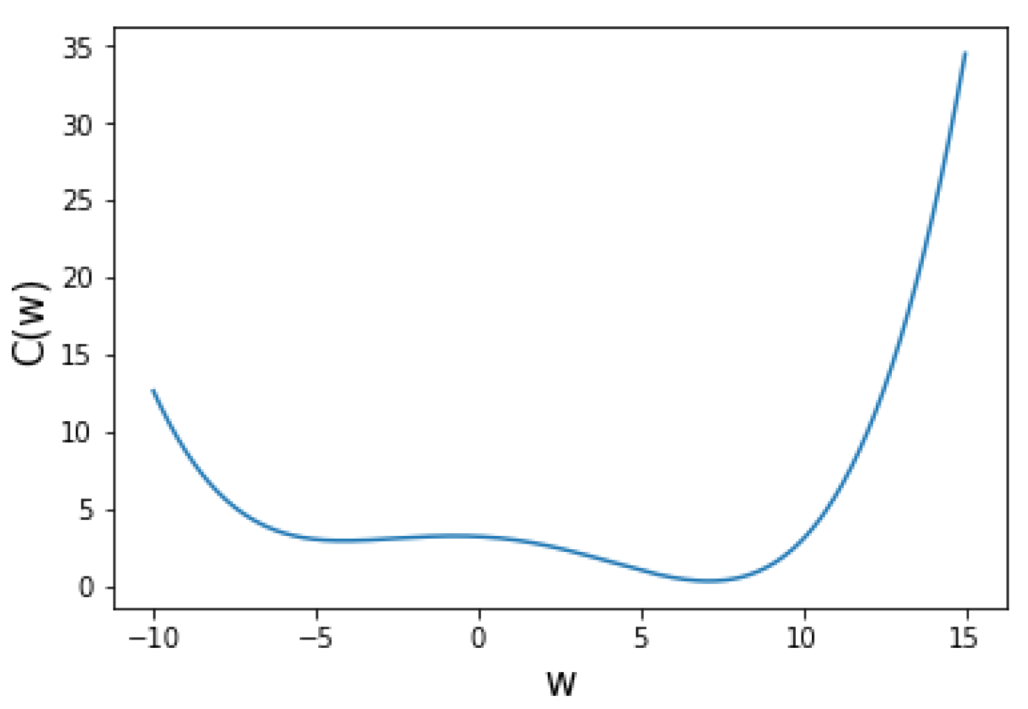
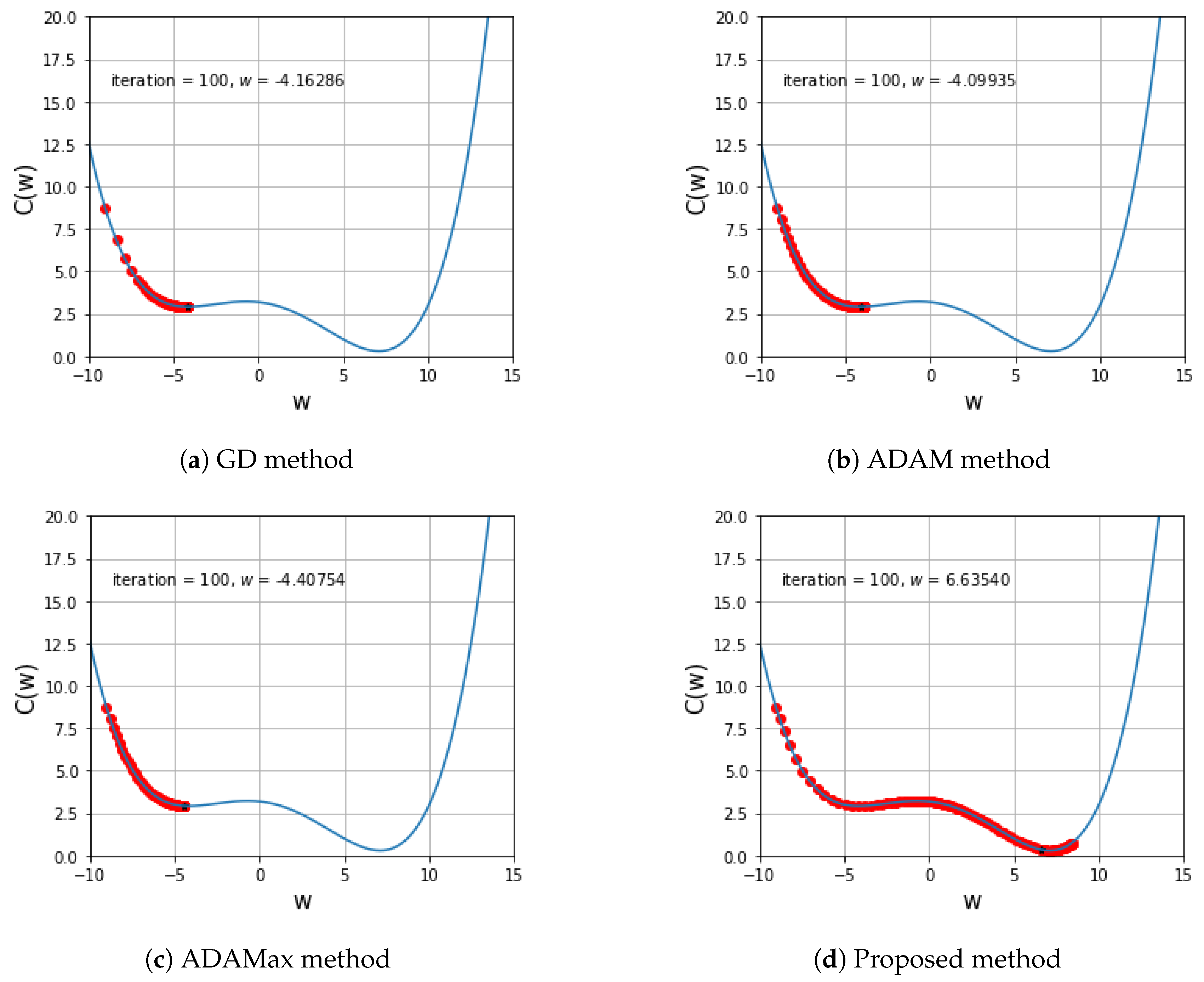
5.1. One Variable Non-Convex Function Test

Since the cost function has a non-convex property, we test each method with a simple non-convex function in this experiment. The cost function is $C\left(w\right)=(w+5)(w+3)(w-1)(w-10)/800+3$ and has the global minimum at $w\approx 7.1047$. The starting point, $w_0$, is initialized at $-9$ and the iteration number is 100. The reason this cost function is divided by 800 is that if you do not divide it, the degree of this function is 4, so the value of the function becomes too big and it is too far away from the real problem.

Figure 2 shows the change in the cost function ($C\left(w\right)$) according to the change in w.

Figure 3 shows the iterations of four methods over $C\left(w\right)$ with $w_0=-9$. In this experiment, GD, ADAM, and AdaMax fall into a local minimum and it is confirmed that there is no motion. On the other hand, the proposed method is confirmed to settle at the global minimum beyond the local minimum. Although the global minimum is near 7, the other methods stayed near $-4$.

5.2. Two Variables Non-Convex Function Test

In this section, we experiment with three two-variable cost functions. The first and second experiments are to find the global minimum of the Beale function and the Styblinski–Tang function, respectively, and the third experiment is to test whether the proposed method works effectively at the saddle point.

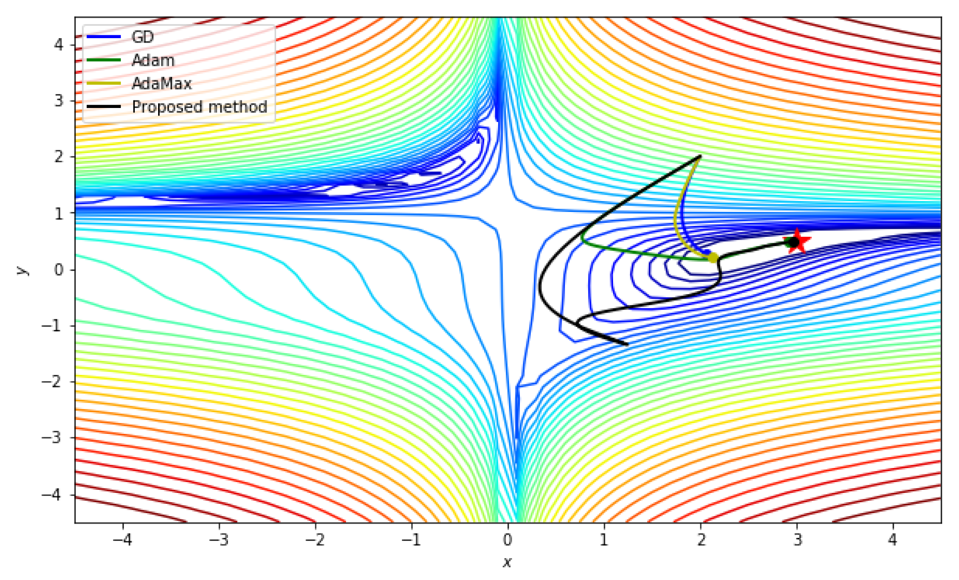
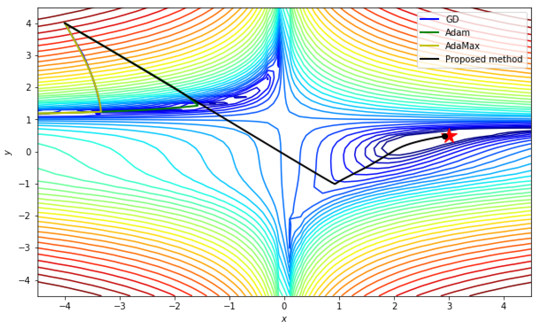
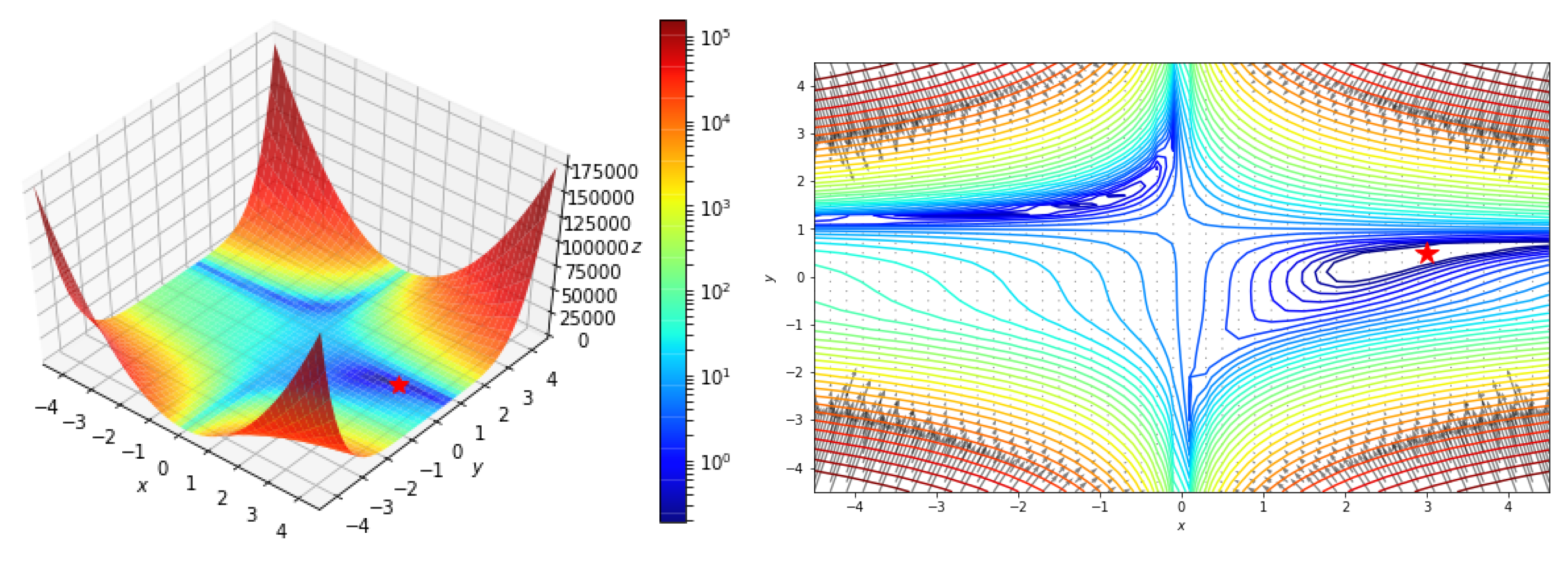
5.2.1. Beale function

The Beale function is defined by $C(w_1,w_2)={(1.5-w_1+w_1{w}_2)}^2+{(2.25-w_1+w_1{w}_2^2)}^2+{(2.625-w_1+w_1{w}_2^3)}^2$ and has the global minimum at (3, 0.5). Figure 4 shows the Beale function.

Figure 5 shows the results of each method. GD’s learning late was set to ${10}^{-4}$, which is different from other methods because only GD has a very large gradient and weight divergence. We confirm that all methods converge well because this function is convex around the given starting point.

Table 1. Change of weights of each method.

Iteration/Method	GD	ADAM	ADAMax	Proposed Method
0	[2.0, 2.0]	[2.0, 2.0]	[2.0, 2.0]	[2.0, 2.0]
100	[1.81, 0.84]	[1.53, 0.24]	[1.75, 0.69]	[2.11, −0.33]
200	[1.85, 0.63]	[2.20, 0.18]	[1.80, 0.53]	[2.50, 0.32]
300	[1.89, 0.52]	[2.39, 0.28]	[1.85, 0.42]	[2.72, 0.41]
400	[1.92, 0.45]	[2.53, 0.34]	[1.90, 0.35]	[2.81, 0.44]
500	[1.95, 0.39]	[2.64, 0.39]	[1.94, 0.30]	[2.87, 0.46]
600	[1.98, 0.35]	[2.73, 0.42]	[1.99, 0.26]	[2.91, 0.47]
700	[2.00, 0.32]	[2.79, 0.44]	[2.03, 0.23]	[2.93, 0.48]
800	[2.03, 0.30]	[2.84, 0.45]	[2.06, 0.22]	[2.95, 0.48]
900	[2.05, 0.28]	[2.88, 0.46]	[2.10, 0.21]	[2.96, 0.49]
1000	[2.06, 0.27]	[2.91, 0.47]	[2.13, 0.21]	[2.97, 0.49]

shows the weight change of each method according to the change of iteration. As you can see from this table, the proposed method shows the best performance.

To see the results from another starting point, we experiment with the same cost function using a different starting point $(-4,4)$, hyperparameter $\lambda =-0.2$ and the iteration number = 50,000.

Figure 6 shows the results of each method. In this experiment, we confirm that GD, ADAM, and AdaMax fall into a local minimum and stop there, whereas the proposed method reaches the global minimum effectively.

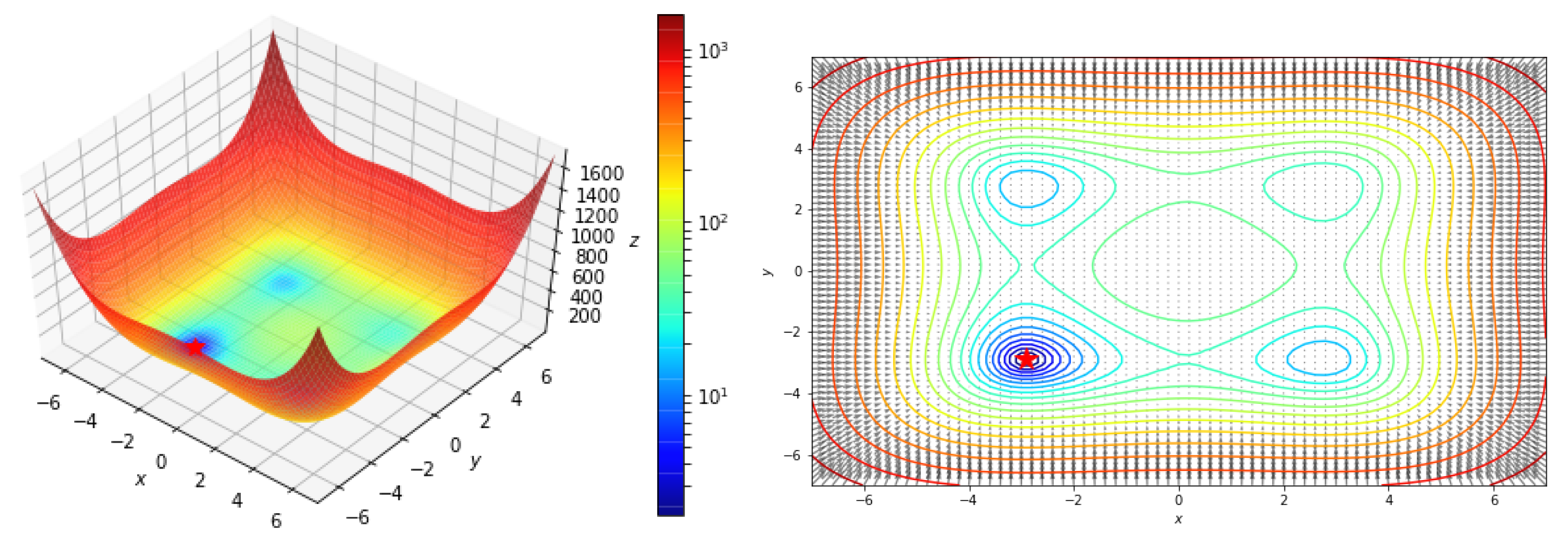
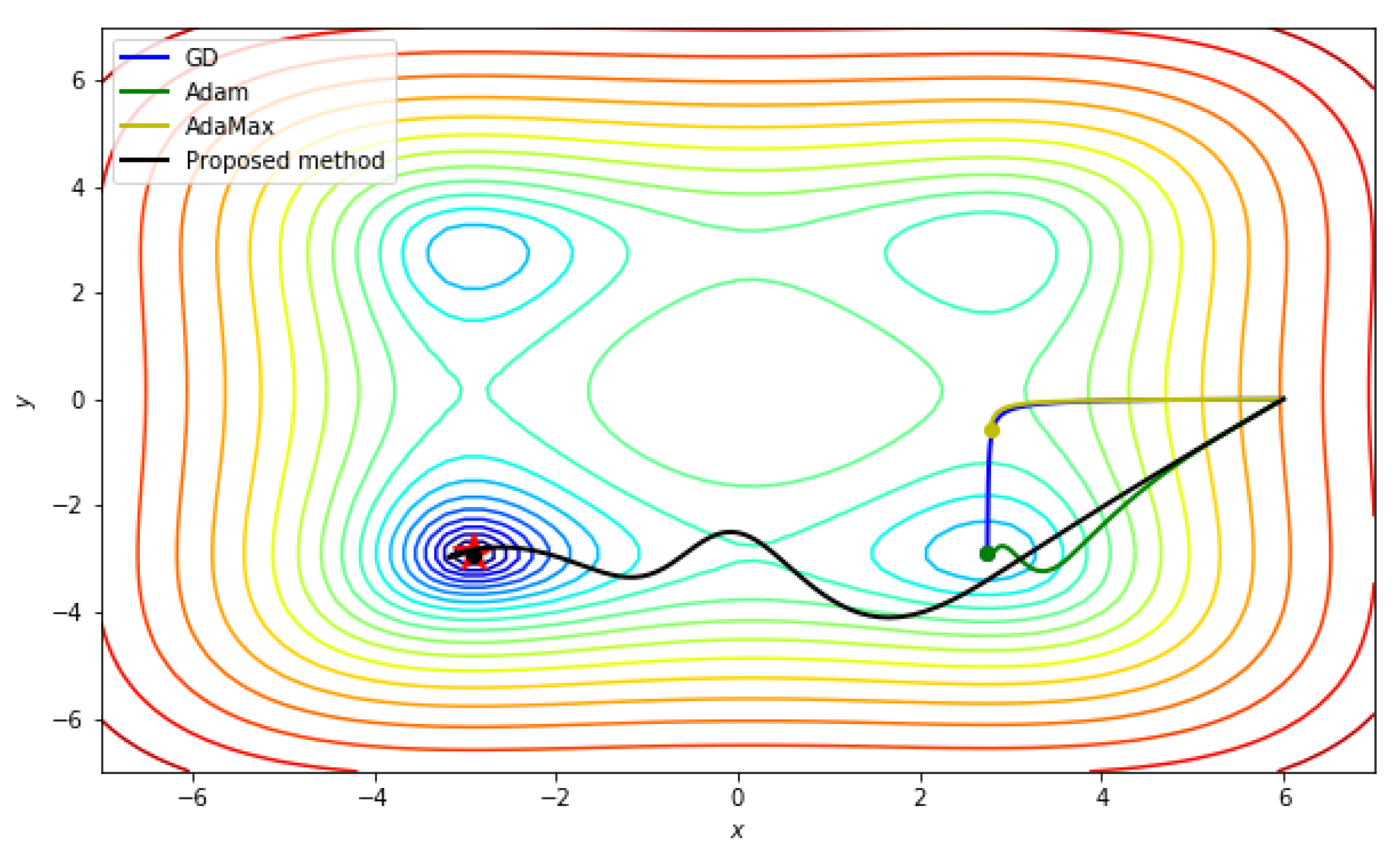
5.2.2. Styblinski–Tang function

The Styblinski–Tang function is defined by

$$C(w_1,w_2)=\left((w_1^4-16w_1^2+5w_1)+{(w_2^4-16w_2^2+5w_2)}^2\right)/2+80$$

and has the global minimum at $(-2.903534,-2.903534)$.

Figure 7 shows the Styblinski–Tang function. In this experiment, we present a result with the starting point $W_0=(6,0)$. Please note that a local minimum point $\approx (2.7468,-2.9035)$ is located between $W_0$ and the global minimum point.

Figure 8 shows the results of each method. Only the Proposed method find the global minimum, and other methods could not avoid a local minimum.

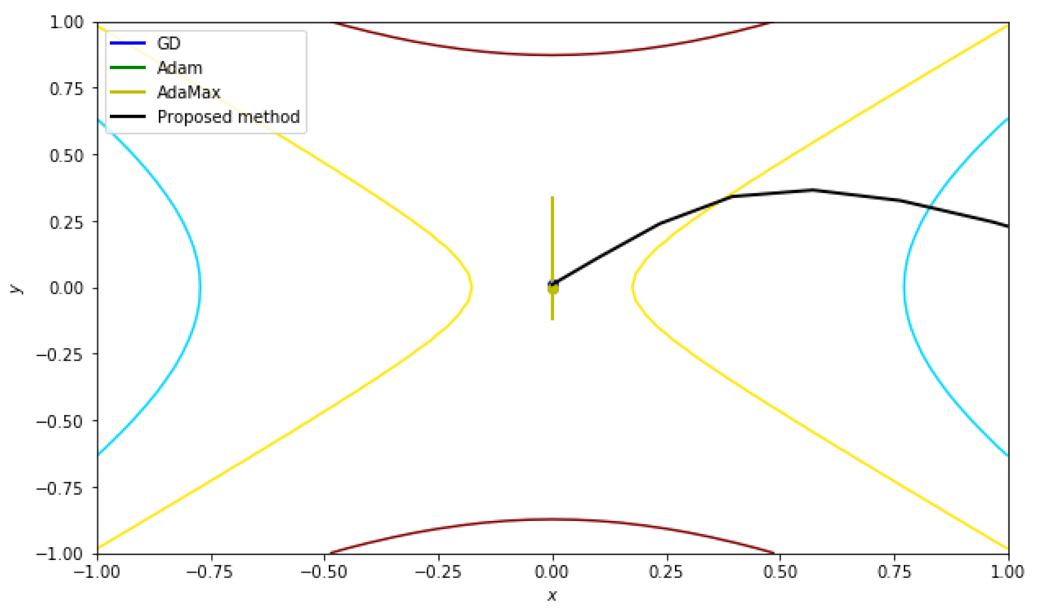
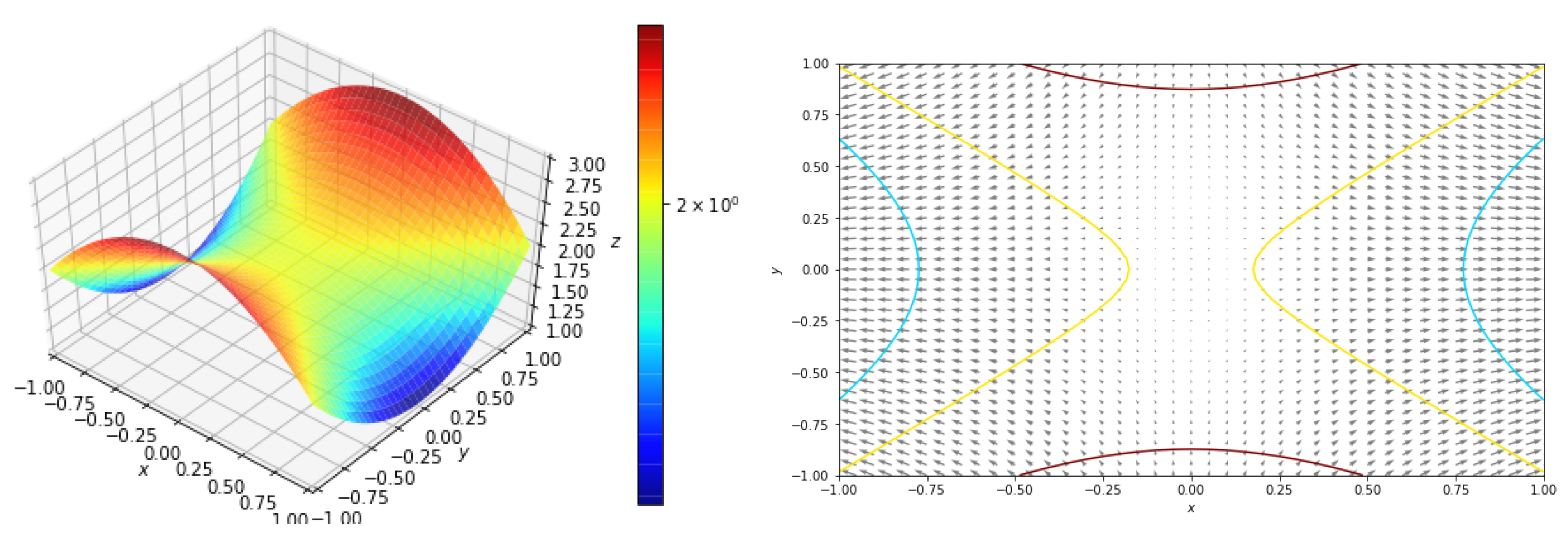
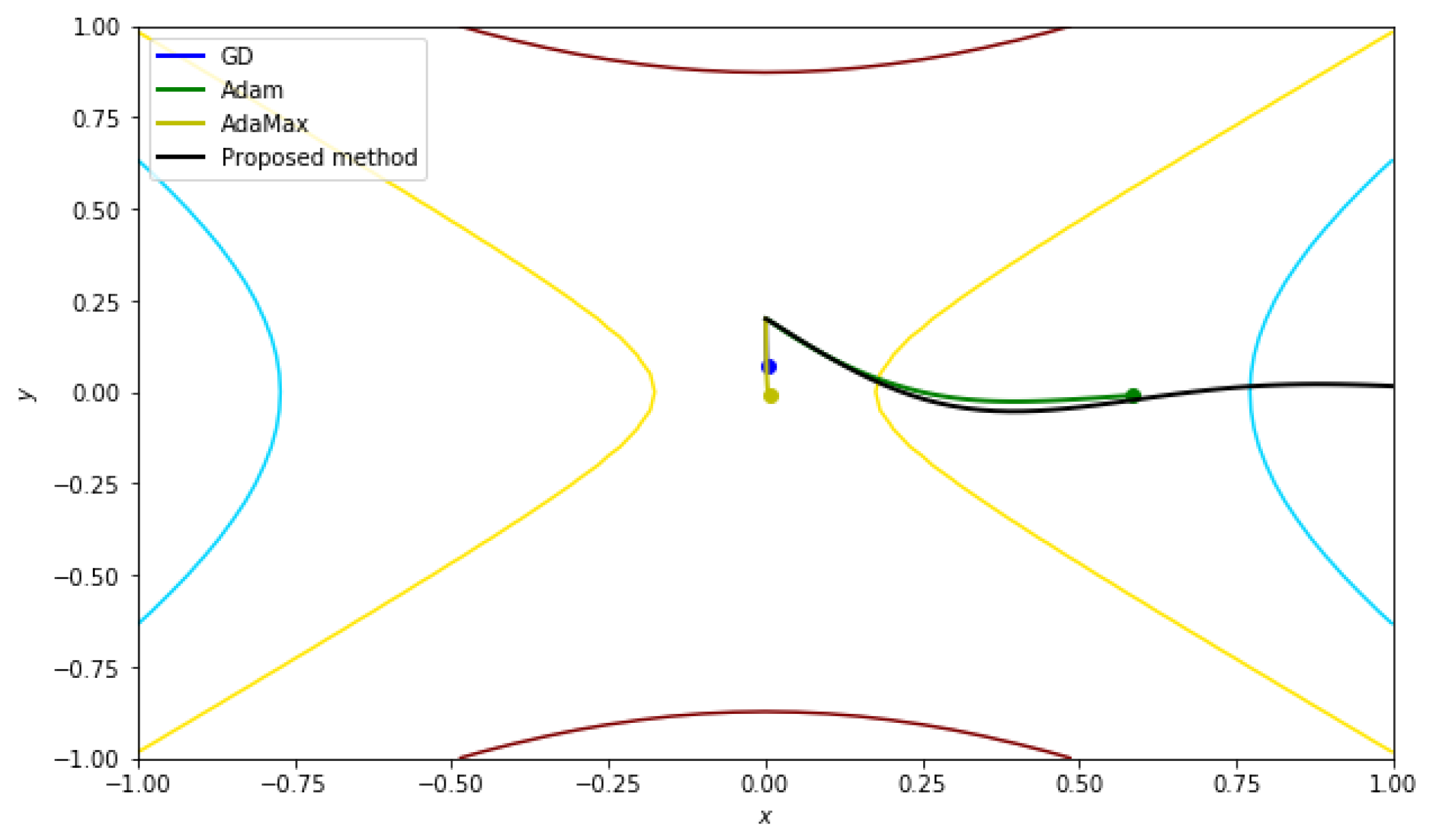
5.2.3. Function with a Saddle Point

The cost function $C(w_1,w_2)=w_2^2-w_1^2+2$ is shown in Figure 9. A Hessian matrix of this cost function is $\left(\begin{array}{cc}-2& 0\\ 0& 2\end{array}\right)$, so this cost function has a saddle point at (0, 0).

In this experiment, we present results based on two different starting points. The first starting point is $W_0=(0.001,0.2)$.

Figure 10 and

Table 2. Change values of each method.

B	GD	ADAM	ADAMax	Proposed Method
0	$[0.001,0.2]$	$[0.001,0.2]$	$[0.001,0.2]$	$[0.001,0.2]$
10	$[0.00121899,0.16341456]$	$[0.0943284,0.10245869]$	$[0.00157076,0.11185508]$	$[0.16787479,0.03591625]$
20	$[0.00148595,0.13352159]$	$[0.20284632,0.02224525]$	$[0.00235688,0.05096114]$	$[0.38849311,-0.05289886]$
30	$[0.00181136,0.10909686]$	$[0.32453918,-0.02053808]$	$[0.00347925,0.0150328]$	$[0.61448606,-0.01491036]$
40	$[0.00220804,0.08914008]$	$[0.45704978,-0.0233784]$	$[0.00511317,-0.00198256]$	$[0.83303301,0.02029141]$
50	$[0.00269159,0.07283394]$	$[0.59806857,-0.0075764]$	$[0.007516,-0.00722015]$	$[1.04047722,0.01258689]$

shows the results of each method. In this experiment, we see that the proposed method also changes the parameters more rapidly than the other three methods near the saddle point.

Then, we performed an experiment with the same cost function, but with another starting point (0, 0.01), and with an iteration number of 100. The hyper parameters in this experiment are the same as above. The only thing that was changed was the starting point.

Figure 11 shows the result of this experiment with an initial point of (0, 0.01). In this experiment, since one of the coordinates of the initial value is 0, the other methods do not work.

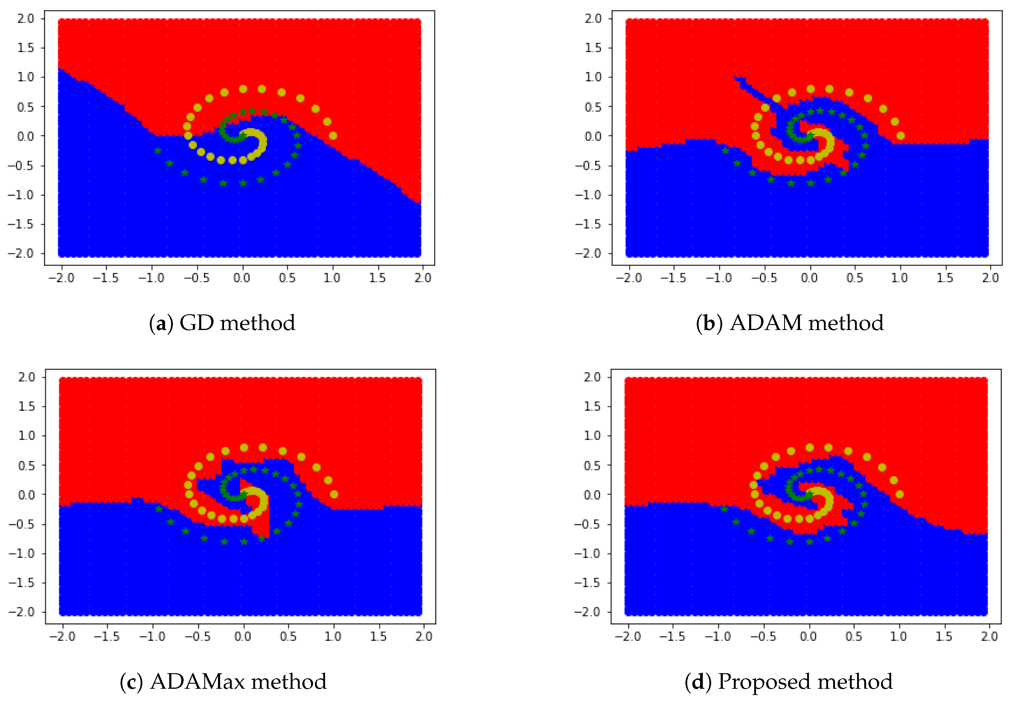
5.3. Two-Dimensional Region Segmentation Test

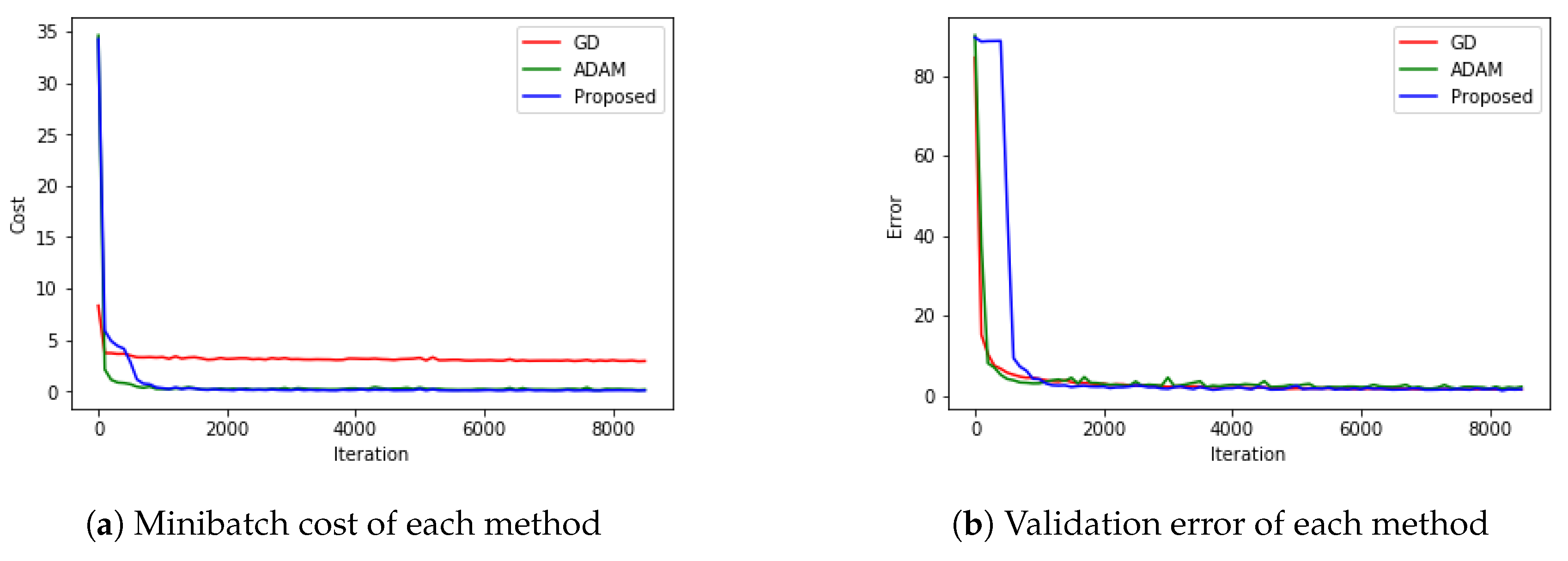
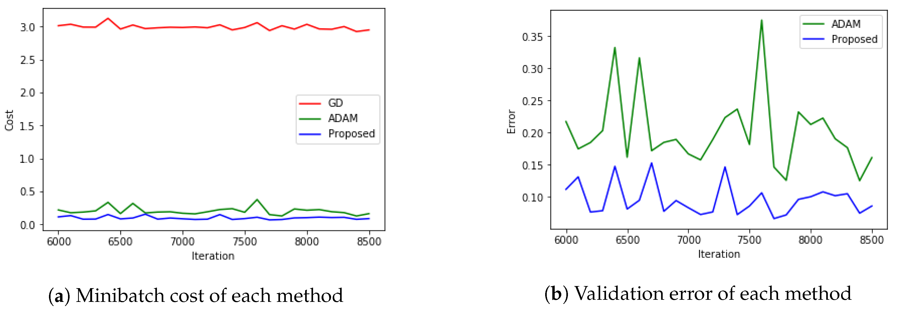
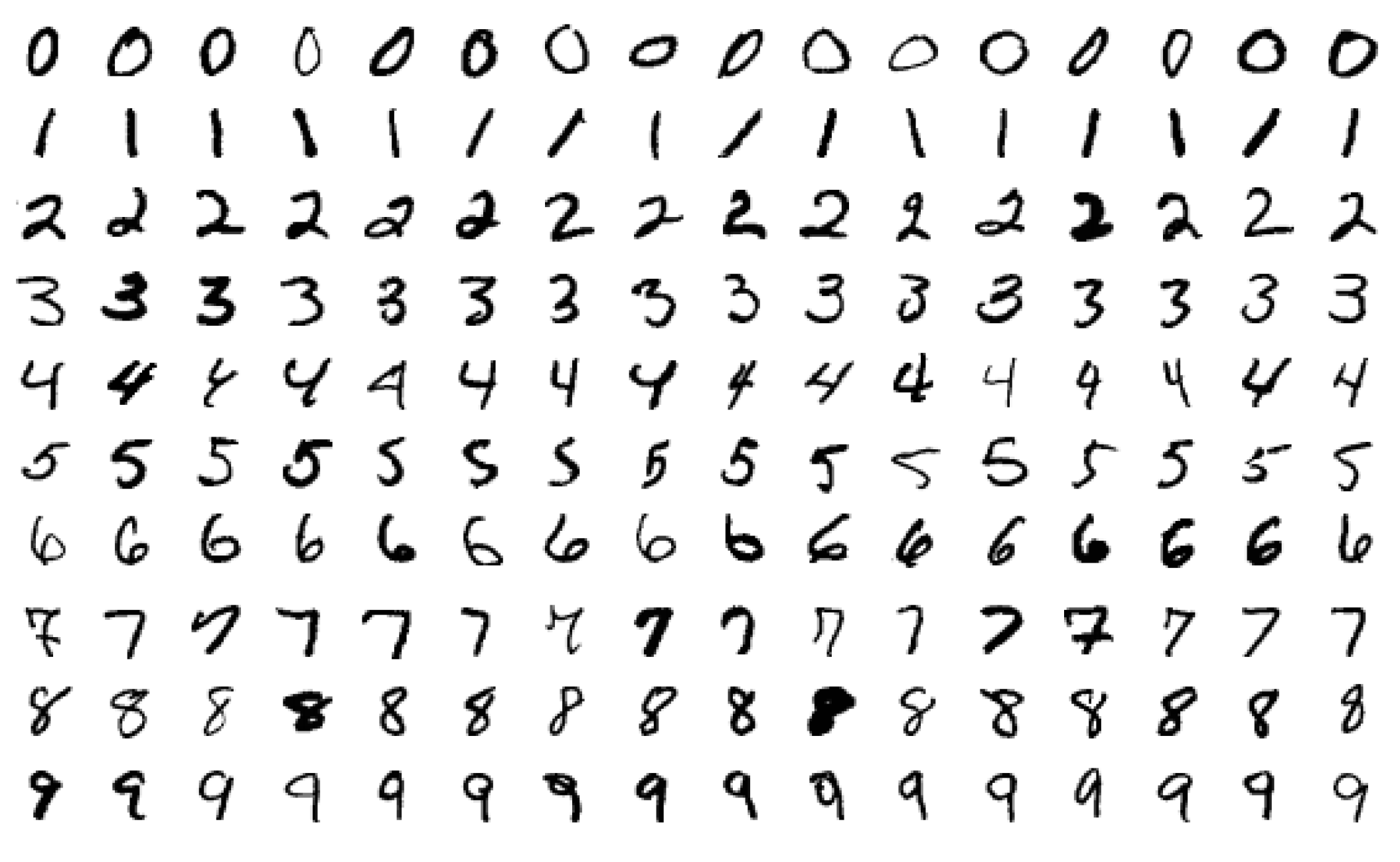
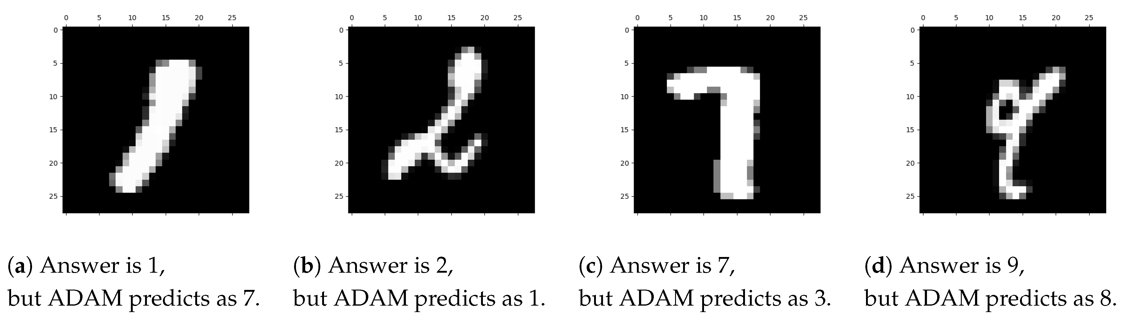
To see how one can divide the area in a more complicated situation, we introduce a problem of region separation in the form of the shape of a whirlwind. The value of 0 and 1 are given along the shape of the whirlwind, and the regions are divided by learning according to each method.

Table 3. Learning dataset.

(a) Image of $\mathit{L}\mathit{S}$	(b) Pseudo code of $\mathit{L}\mathit{S}$
	$LS$: empty set for i = 1: 30 $r=5i/30$ $t=5\pi i/30$ $\left(\right[rsin\left(t\right),rcos\left(t\right)],1)$ put in $LS$ end for for i = 1: 30 $r=5i/30$ $t=5\pi i/30$ + $\pi$ $\left(\right[rsin\left(t\right),rcos\left(t\right)],0)$ put in $LS$ end for return $LS$

b is the pseudo code for making the learning dataset for this experiment and Table 3a is a visualization of the dataset.

To solve this problem, we use a 2-layer and 25-row neural network. First, the neural network is learned by each method. After that, $[-2,2]\times [-2,2]$ is divided into 60 equal sections, and each of the 3600 coordinates are checked to decide the parts where they belong.

The results are presented in Figure 12. The proposed method is better expressed in dividing the region according to the direction of the whirlwind, compared with other schemes.

In the same artificial neural network structure, different results were obtained for each method, which is related to the accuracy of location learning.

5.4. MNIST with CNN

In the previous sections, we have seen simple cases of classification problems using ANN. Here, we try a more practical experiment using a CNN (Convolutional Neural Network). As we all know, we use an ANN to increase the number of layers to solve more difficult and complex problems. However, as the number of layers increases, the number of parameters also increases, and the memory and operating time of the computer, likewise, also increase. For this reason, a CNN was introduced and the performance is shown at The ImageNet Large Scale Visual Recognition Challenge (ILSVRC) [11]. Therefore, in this experiment, we want to see how our method works with the CNN structure. In this experiment, TensorFlow was used, and for the fairness of the experiment, we used the MNIST problem using a CNN, which is one of the basic examples provided in TensorFlow (see https://github.com/tensorflow/models/tree/master/tutorials/image/mnist). There were 8600 iterations, which output the Minibatch cost and validation error of each method as a result. The results are shown in Figure 13. As shown in Figure 13, all methods were found to reduce both cost and error.

For further investigation, we magnify the data from Figure 13 from the 6000th iteration, and show it in Figure 14.

Figure 14a shows that GD converges the slowest and the proposed method is more accurate than ADAM. Figure 14b shows the accuracies of the proposed method and the ADAM method, as measured on the test data. From this, we see that the proposed method works better for the classification of images than ADAM.

Figure 15 shows four sample digits from the MNIST test data that the proposed method classifies effectively but that ADAM failed to classify in this experiment.

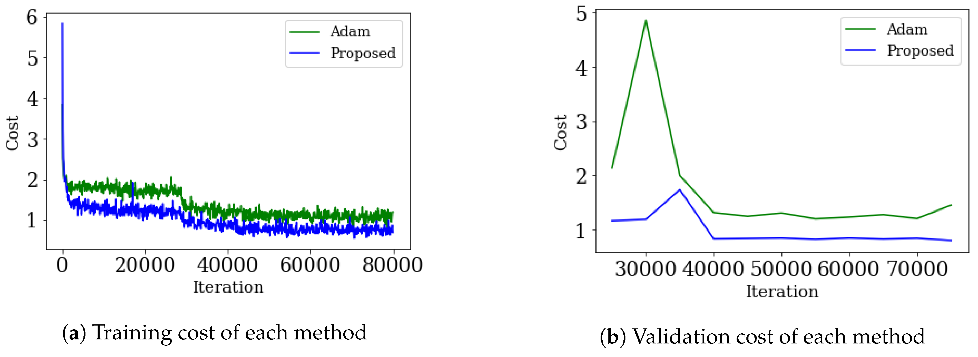
5.5. CIFAR-10 with RESNET

We show in Section 5.4 that the proposed method is more effective than ADAM in the CNN structure using the MNIST dataset. Since the MNIST dataset is a grayscale image, the size of one image is $28\times 28\times 1$. In this section, we show that the proposed method is more effective than ADAM when using a dataset larger than the MNIST, such as the CIFAR10 (https://www.cs.toronto.edu/~kriz/cifar.html). CIFAR10 is a popular dataset for classifying 10 categories (airplane, automobile, bird, cat, deer, dog, frog, horse, ship, and truck) $32\times 32\times 3$ size RGB images. This dataset consists of 50,000 training data and 10,000 test data. In this experiment, as in Section 5.4, we used the example code (the same model and the same hyperparameter settings) provided by TensorFlow (see https://github.com/tensorflow/models/tree/master/tutorials/image/cifar10_estimator). In Section 5.4, we used a simple network using a CNN, but in this subsection, we use a more complex and high-performance network called RESNET (Residual network) based on CNN. RESNET is a well-known network that has good performance in ILSVRC, and we used RESNET 44 in this experiment.

Figure 16 shows the results of the training CIFAR10 dataset using the RESNET structure, and are compared with ADAM. In Figure 16a, the training cost of each method was calculated and plotted every 100th iteration. In Figure 16b, the validation cost of each method was calculated and plotted every 5000th iteration. This shows that the proposed method works effectively for more complex networks as well as simple networks.

6. Conclusions

In this paper, we propose a new optimization method based on ADAM. Many of the existing optimization methods (including ADAM) may not work properly according to the initial point. However, the proposed method finds the global minimum better than other methods, even if there is a local minimum near the starting point, and has better overall performance. We tested our method only on models for image datasets such as MNIST and CIFAR10. Our future work is to test our method on various models such as RNN models for time series prediction, various models for natural language processing, etc.

References

1. Deng, L.; Li, J.; Huang, J.; Yao, K.; Yu, D.; Seide, F.; Seltzer, M.L.; Zweig, G.; He, X.; Williams, J.; et al. Recent advances in deep learning for speech research at microsoft. In Proceedings of the 2013 IEEE International Conference on Acoustics, Speech and Signal Processing—ICASSP 2013, Vancouver, BC, Canada, 26–31 May 2013. [Google Scholar]
2. Graves, A. Generating sequences with recurrent neural networks. arXiv 2013, arXiv:1308.0850. [Google Scholar]
3. Graves, A.; Mohamed, A.; Hinton, G. Speech recognition with deep recurrent neural networks. In Proceedings of the 2013 International Conference on Acoustics, Speech and Signal Processing—ICASSP 2013, Vancouver, BC, Canada, 26–31 May 2013; pp. 6645–6649. [Google Scholar]
4. Hinton, G.E.; Srivastava, N.; Krizhevsky, A.; Sutskever, I.; Salakhutdinov, R.R. Improving neural networks by preventing co-adaptation of feature detectors. arXiv 2012, arXiv:1207.0580. [Google Scholar]
5. Tieleman, T.; Hinton, G.E. Lecture 6.5—RMSProp, COURSERA: Neural Networks for Machine Learning; Technical Report; COURSERA: Mountain View, CA, USA, 2012. [Google Scholar]
6. Dean, J.; Corrado, G.; Monga, R.; Chen, K.; Devin, M.; Le, Q.; Mao, M.; Ranzato, M.; Senior, A.; Tucker, P.; et al. Large scale distributed deep networks. In Proceedings of the 25th International Conference on Neural Information Processing Systems—NIPS 2012, Lake Tahoe, NV, USA, 3 December 2012; pp. 1223–1231. [Google Scholar]
7. Jaitly, N.; Nguyen, P.; Senior, A.; Vanhoucke, V. Application of pretrained deep neural networks to large vocabulary speech recognition. In Proceedings of the INTERSPEECH 2012, 13th Annual Conference of the International Speech Communication Association—ISCA 2012, Portland, OR, USA, 9–13 September 2012; pp. 2578–2581. [Google Scholar]
8. Amari, S. Natural gradient works efficiently in learning. Neural Comput. 1998, 10, 251–276. [Google Scholar] [CrossRef]
9. Duchi, J.; Hazan, E.; Singer, Y. Adaptive subgradient methods for online learning and stochastic optimization. J. Mach. Learn. Res. 2011, 12, 2121–2159. [Google Scholar]
10. Hinton, G.; Deng, L.; Yu, D.; Dahl, G.E.; Mohamed, A.; Jaitly, N.; Senior, A.; Vanhoucke, V.; Nguyen, P.; Sainath, T.N. Deep neural networks for acoustic modeling in speech recognition: The shared views of four research groups. Signal Process. Mag. 2012, 29, 82–97. [Google Scholar] [CrossRef]
11. Krizhevsky, A.; Sutskever, I.; Hinton, G.E. Imagenet classification with deep convolutional neural networks. In Proceedings of the Neural Information Processing Systems–NIPS 2012, Lake Tahoe, NV, USA, 3 December 2012; pp. 1097–1105. [Google Scholar]
12. Pascanu, R.; Bengio, Y. Revisiting natural gradient for deep networks. arXiv 2013, arXiv:1301.3584. [Google Scholar]
13. Sutskever, I.; Martens, J.; Dahl, G.; Hinton, G.E. On the importance of initialization and momentum in deep learning. In Proceedings of the 30th International Conference on Machine Learning—ICML 2013, Atlanta, GA, USA, 16–21 Jun 2013; PMLR 28(3). pp. 1139–1147. [Google Scholar]
14. Kochenderfer, M.; Wheeler, T. Algorithms for Optimization; The MIT Press Cambridge: London, UK, 2019. [Google Scholar]
15. Kingma, D.P.; Ba, J. ADAM: A method for stochastic optimization. In Proceedings of the 3rd International Conference for Learning Representations—ICLR 2015, San Diego, CA, USA, 7–9 May 2015. [Google Scholar]
16. Bottou, L.; Curtis, F.E.; Nocedal, J. Optimization Methods for Large-Scale Machine Learning. SIAM Rev. 2018, 60, 223–311. [Google Scholar] [CrossRef]
17. Roux, N.L.; Fitzgibbon, A.W. A fast natural newton method. In Proceedings of the 27th International Conference on Machine Learning—ICML 2010, Haifa, Israel, 21–24 June 2010; pp. 623–630. [Google Scholar]
18. Sohl-Dickstein, J.; Poole, B.; Ganguli, S. Fast large-scale optimization by unifying stochastic gradient and quasi-newton methods. In Proceedings of the 31st International Conference on Machine Learning—ICML 2014, Beijing, China, 21–24 June 2014; pp. 604–612. [Google Scholar]
19. Zeiler, M.D. Adadelta: An adaptive learning rate method. arXiv 2012, arXiv:1212.5701. [Google Scholar]
20. Rumelhart, D.E.; Hinton, G.E.; Williams, R.J. Learning representations by back-propagating errors. Nature 1986, 323, 533–536. [Google Scholar] [CrossRef]
21. Becker, S.; LeCun, Y. Improving the Convergence of Back-Propagation Learning with Second Order Methods; Technical Report; Department of Computer Science, University of Toronto: Toronto, ON, Canada, 1988. [Google Scholar]
22. Kelley, C.T. Iterative methods for linear and nonlinear equations. In Frontiers in Applied Mathematics; SIAM: Philadelphia, PA, USA, 1995; Volume 16. [Google Scholar]
23. Reddi, S.J.; Kale, S.; Kumar, S. On the Convergence of ADAM and Beyond. arXiv 2019, arXiv:1904.09237. [Google Scholar]
24. Ruppert, D. Efficient Estimations from a Slowly Convergent Robbins-Monro Process; Technical Report; Cornell University Operations Research and Industrial Engineering: Ithaca, NY, USA, 1988. [Google Scholar]
25. Zinkevich, M. Online Convex Programming and Generalized Infinitesimal Gradient Ascent. In Proceedings of the Twentieth International Conference on Machine Learning—ICML-2003, Washington, DC, USA, 21–24 August 2003; pp. 928–935. [Google Scholar]
Figure 1. Examples of MNIST dataset.
Applsci 10 01073 g001
Figure 2. Cost function with one local minimum.
Applsci 10 01073 g002
Figure 3. Compared to the other scheme, the learning rate is 0.2 and the β 1 , β 2 , λ used in the proposed method are 0.95, 0.9999, 10 2 .
Applsci 10 01073 g003
Figure 4. Beale Function.
Applsci 10 01073 g004
Figure 5. Result of the Beale function with an initial point of (2, 2). W 0 = ( 2 , 2 ) and the iteration number are 1000. The learning rate is 0.1 and the β 1 , β 2 , and λ used in proposed method are 0.9, 0.999, and 0.5 , respectively. GD’s learning late was set to 10 4 .
Applsci 10 01073 g005
Figure 6. Result of Beale function with initial point ( 4 , 4 ) .
Applsci 10 01073 g006
Figure 7. Styblinski–Tang Function.
Applsci 10 01073 g007
Figure 8. Result of Styblinski–Tang function with initial point ( 6 , 0 ) . The learning rate is 0.1 and the β 1 , β 2 , λ used in Proposed method are 0.95, 0.9999, 0.2 and GD’s learning late was set to 10 3 .
Applsci 10 01073 g008
Figure 9. Cost function C ( w 1 , w 2 ) = w 2 2 w 1 2 + 2 .
Applsci 10 01073 g009
Figure 10. The results near the saddle point with an initial point of (0.001, 2). The iteration number is 50, the learning rate is 10 2 , and the β 1 , β 2 , and λ used in the proposed method are 0.95, 0.9999, and 5 × 10 3 , respectively.
Applsci 10 01073 g010
Figure 11. The result of the saddle point with an initial point of (0, 0.01).
Applsci 10 01073 g011
Figure 12. Comparing proposed scheme with other schemes.
Applsci 10 01073 g012
Figure 13. Comparing the proposed scheme with other schemes.
Applsci 10 01073 g013
Figure 14. Comparing the proposed scheme with other schemes with an iteration number over 6000.
Applsci 10 01073 g014
Figure 15. Examples that the proposed method predicted correctly, while the ADAM method does not.
Applsci 10 01073 g015
Figure 16. Result of CIFAR10 dataset using the RESNET 44 model. The following parameters are default values; iteration: 80000, batch size: 128,weight decay: 2 × 10 4 ,learning rate: 0.1, batch norm decay: 0.997.
Applsci 10 01073 g016