Analysis and Modeling of Timbre Perception Features in Musical Sounds

 and
and
Abstract
1. Introduction
2. Timbre Database Construction
2.1. Timbre Material Collection
2.2. Loudness Normalization
3. Construction of the Timbre Subjective Evaluation Term System
3.1. Construction of the Thesaurus for Timbre Evaluation Terms
3.2. Experiment A: A Subjective Evaluation Experiment Based on a Forced Selection Methodology
3.3. Data Analysis and Conclusion of Experiment A
4. Construction of a Timbre Perception Feature Model
4.1. Construction of the Objective Acoustic Parameter Set
- (1)
- Temporal shape features: calculated from the waveform or the signal energy envelope (e.g., attack-time, temporal increase or decrease, and effective duration).
- (2)
- Temporal features: auto-correlation coefficients with a zero-crossing rate.
- (3)
- Energy features: referring to various energy content in the signal (i.e., global energy, harmonic energy, or noise energy).
- (4)
- Spectral shape features: calculated from the short-time Fourier transform (STFT) of the signal (e.g., centroid, spread, skewness, kurtosis, slope, roll-off frequency, or Mel-frequency cepstral coefficients).
- (5)
- Harmonic features: calculated using sinusoidal harmonic modeling of the signal (e.g., harmonic/noise ratio, odd-to-even and tristimulus harmonic energy ratio, and harmonic deviation).
- (6)
- Perceptual features: calculated using a model of human hearing (i.e., relative specific loudness, sharpness, and spread).
4.2. Calculation Method
4.3. Experiment B: A Timbre Evaluation Experiment Based on the Method of Successive Categories
4.4. Construction of a Prediction Model
- (1)
- Screening: removes unimportant or problematic predictors and cases.
- (2)
- Ranking: sorts remaining predictors and assigns ranks; this step considers one predictor at a time to determine how well it predicts the target variable.
- (3)
- Selecting: identifies the important subset of features to use in subsequent models.
5. The Construction of Timbre Space
- (1)
- Subjective evaluation experiment based on sample dissimilarity: where a dissimilarity matrix between samples was obtained using a subjective evaluation experiment. Existing research has conventionally paired up samples in the material database to score the dissimilarity. The process was simplified in this study, which reduced the workload.
- (2)
- Dimension reduction of distance matrix based on MDS: where the MDS algorithm was used to calculate the dissimilarity matrix such that sample distances in high-dimensional spaces can be represented in low-dimensional spaces (usually two or three dimensions).
- (3)
- Attribute interpretation of each dimension of timbre space: where the correlation between each dimension and the timbre perception features was analyzed using a statistical method. Interpretable attributes for each dimension were then acquired from this space.
5.1. Experiment C: Subjective Evaluation Experiment Based on Sample Dissimilarity
- (1)
- The appropriate number of samples: The number of samples must be sufficiently large to ensure the accuracy of the MDS algorithm and impose sufficient constraints on the model. In practice, however, it is difficult to establish precise rules for determining these data. However, empirical solutions do exist. In most MDS-based timbre studies, at least 10 sound samples are required for two-dimensional spaces and at least 15 sound samples are needed for three-dimensional spaces [51,74,75]. In this paper, 37 kinds of Chinese instruments were used as experimental materials, which ensured that sufficient constraints were provided to the MDS model.
- (2)
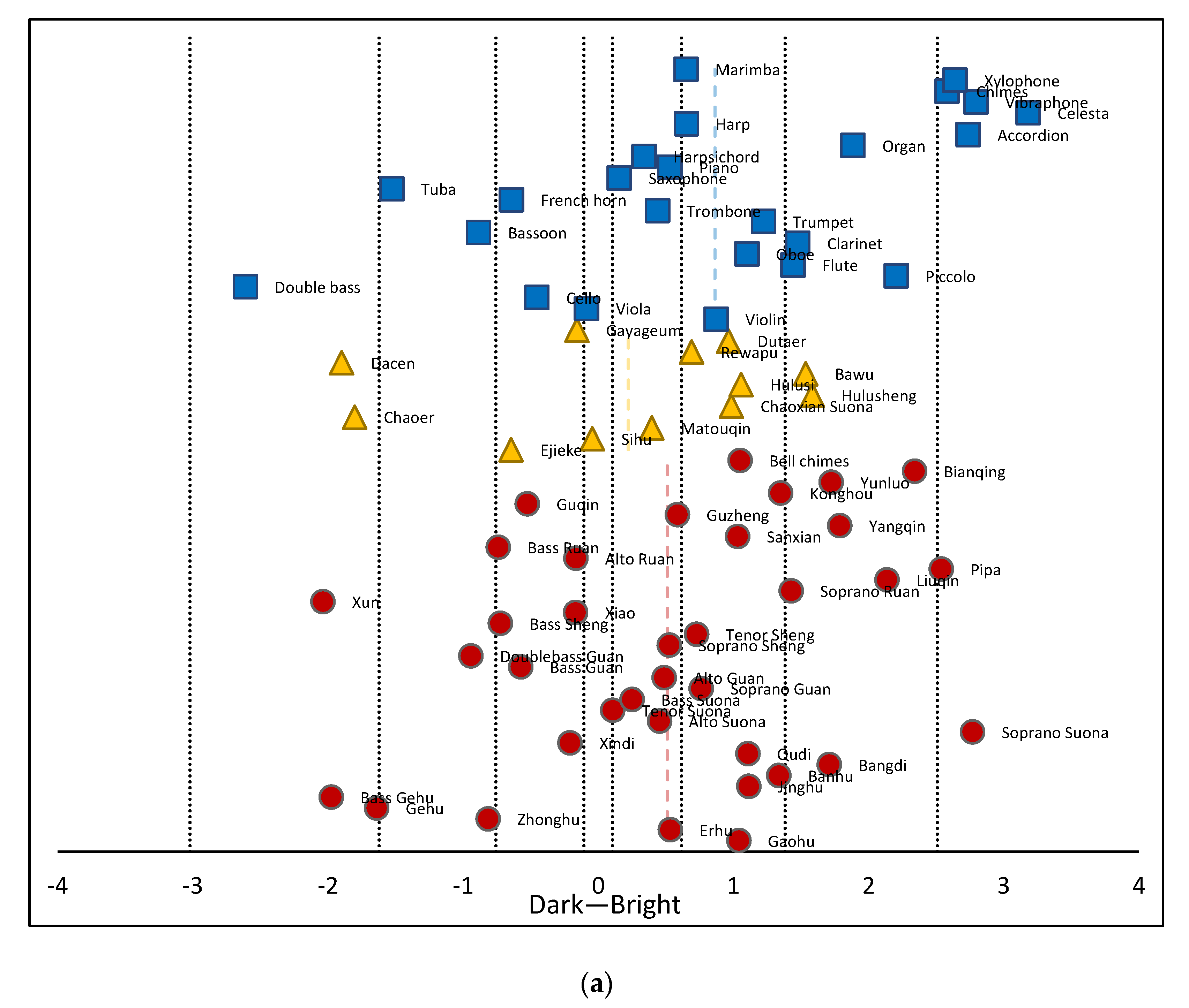
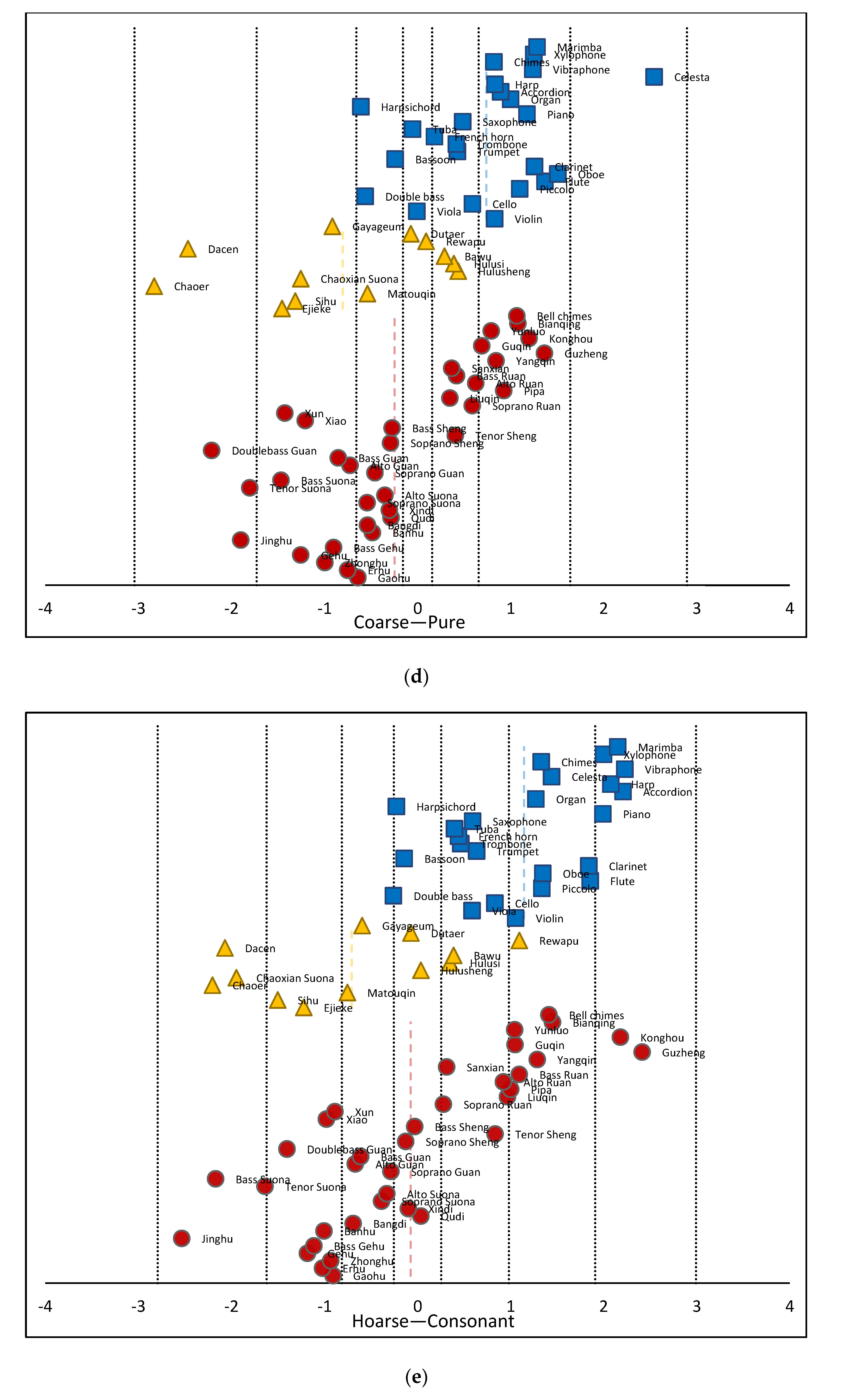
- The range of timbre variation: The range of timbre varies depending on the subject of the study, with larger instrumental variety (i.e., orchestral music) providing better data [34]. Models constructed in this way can be applied more broadly to new timbre samples. In this study, 37 kinds of Chinese instruments were selected. As can be seen from Figure 4, compared with Western instruments, Chinese instruments had a wider distribution range in terms of their timbre evaluation scale. As such, the Chinese instrument samples selected in this paper ensured a diverse range of timbre samples.
- (3)
- The uniformity of timbre sample distributions: The distribution of sound samples in each timbre perception attribute should be as uniform as possible. Timbre spaces are continuous perceptual spaces and a uniform distribution sample set is beneficial to the construction of continuous timbre spaces. Non-uniform sample distributions can degrade solutions to the MDS equations, preventing the structures between classes from being fully displayed [76]. As seen in Figure 4, the samples selected in this study covered a broad range of timbre attributes and they were distributed at varying psychological scales, providing a uniform distribution.
5.2. The Construction of the 3D Timbre Space Using MDS
5.3. Perception Attribute Analysis of the Timbre Space Dimension
6. Conclusions
- (1)
- A novel method was proposed for constructing two sets of timbre evaluation terminology systems in a Chinese context. Experimental results from a subjective evaluation showed that these terms could successfully distinguish timbre from different instruments.
- (2)
- A timbre material library containing 72 musical instruments was constructed according to relevant standards. A subjective evaluation experiment was conducted using the method of successive categories. The psychological scales of the subjects were acquired using five pairs of perceptual dimensions. A mathematical model of timbre perception features was then developed using multiple linear regression, support vector regression, a neural network, and the random forest algorithm. Experimental results showed that this constructed model could predict perceptual features for new samples.
- (3)
- An improved method for constructing 3D timbre space was proposed and demonstrated using the MDS algorithm applied to 37 Chinese instruments. Auditory perceptual attributes were determined by analyzing the correlation between the 3 dimensions of the timbre space and 16 perceptual attributes.
Author Contributions
Funding
Conflicts of Interest
Appendix A

| Category | Type | Name of the Instrument | |||
|---|---|---|---|---|---|
| Chinese Orchestral Instruments (37) | Bowed Instrument (7) | 高胡 (Gaohu) | 二胡 (Erhu) | 中胡 (Zhonghu) | 革胡 (Gehu) |
| 低音革胡 (Bass Gehu) | 京胡 (Jinghu) | 板胡 (Banhu) | |||
| Wind Instrument (17) | 梆笛 (Bangdi) | 曲笛 (Qudi) | 新笛 (Xindi) | ||
| 高音笙 (Soprano Sheng) | 中音笙 (Tenor Sheng) | 低音笙 (Bass Sheng) | |||
| 高音唢呐 (Soprano Suona) | 中音唢呐 (Alto Suona) | 次中音唢呐 (Tenor Suona) | 低音唢呐 (Bass Suona) | ||
| 高音管 (Soprano Guan) | 中音管 (Alto Guan) | 低音管 (Bass Guan) | 倍低音管 (Doublebass Guan) | ||
| 埙 (Xun) | 箫 (Xiao) | 巴乌 (Bawu) | |||
| Plucked Instrument (10) | 小阮 (Soprano Ruan) | 中阮 (Alto Ruan) | 大阮 (Bass Ruan) | ||
| 柳琴 (Liuqin) | 琵琶 (Pipa) | 扬琴 (Yangqin) | 古筝 (Guzheng) | ||
| 古琴 (Guqin) | 箜篌 (Konghou) | 三弦 (Sanxian) | |||
| Percussion Instrument (3) | 编钟 (Bell chimes) | 编磬 (Bianqing) | 云锣 (Yunluo) | ||
| Chinese Minority Instruments (11) | Bowed Instrument (4) | 艾捷克 (Ejieke) | 四胡 (Sihu) | 马头琴 (Matouqin) | 潮尔 (Chaoer) |
| Wind Instrument (4) | 朝鲜唢呐 (Chaoxian Suona) | 葫芦笙 (Hulusheng) | 葫芦丝 (Hulusi) | 大岑 (Dacen) | |
| Plucked Instrument (3) | 热瓦普 (Rewapu) | 都塔尔 (Dutaer) | 伽倻琴 (Gayageum) | ||
| Western Orchestral Instruments (24) | Bowed Instrument (4) | Violin | Viola | Cello | Double bass |
| Woodwind Instrument (6) | Piccolo | Flute | Oboe | Clarinet | |
| Bassoon | Saxophone | ||||
| Brass Instrument (4) | Trumpet | Trombone | French horn | Tuba | |
| Keyboard Instrument (4) | Piano | Harpsichord | Organ | Accordion | |
| Plucked Instrument (1) | Harp | ||||
| Percussion Instrument (5) | Celesta | Vibraphone | Chimes | Xylophone | |
| Marimba | |||||
References
- Chen, X. Sound and Hearing Perception; China Broadcasting and Television Press: Beijing, China, 2006. [Google Scholar]
- Moore, B.C.; Glasberg, B.R.; Baer, T. A model for the prediction of thresholds, loudness, and partial loudness. J. Audio Eng. Soc. 1997, 45, 224–240. [Google Scholar]
- Meddis, R.; O’Mard, L. A unitary model of pitch perception. J. Acoust. Soc. Am. 1997, 102, 1811–1820. [Google Scholar] [CrossRef]
- Patel, A.D. Music, Language, and the Brain; Oxford University Press: Oxford, UK, 2010. [Google Scholar]
- ANSI S1.1-1994. American National Standard Acoustical Terminology; Acoustical Society of America: New York, NY, USA, 1994. [Google Scholar]
- Zwicker, E.; Fastl, H. Psychoacoustics: Facts and Models; Springer Science & Business Media: Berlin, Germany, 2013; Volume 22. [Google Scholar]
- Cermak, G.W.; Cornillon, P.C. Multidimensional analyses of judgments about traffic noise. J. Acoust. Soc. Am. 1976, 59, 1412–1420. [Google Scholar] [CrossRef]
- Kuwano, S.; Namba, S.; Fastl, H.; Schick, A. Evaluation of the impression of danger signals-comparison between Japanese and German subjects. In Contributions to Psychological Acoustics; Schick, A., Klatte, M., Eds.; BIS: Oldenburg, Germany, 1997; pp. 115–128. [Google Scholar]
- Iwamiya, S.-I.; Zhan, M. A comparison between Japanese and Chinese adjectives which express auditory impressions. J. Acoust. Soc. Jpn. (E) 1997, 18, 319–323. [Google Scholar] [CrossRef]
- Stepanek, J. Relations between perceptual space and verbal description in violin timbre. acústica 2004 Guimarães 2004, 077. [Google Scholar]
- Kim, S.; Bakker, R.; Ikeda, M. Timbre preferences of four listener groups and the influence of their cultural backgrounds. In Proceedings of the Audio Engineering Society: Audio Engineering Society Convention 140, Paris, France, 4–7 June 2016. [Google Scholar]
- Solomon, L.N. Semantic Approach to the Perception of Complex Sounds. J. Acoust. Soc. Am. 1958, 30, 421–425. [Google Scholar] [CrossRef]
- von Bismarck, G. Timbre of steady sounds: A factorial investigation of its verbal attributes. Acta Acust. United Acust. 1974, 30, 146–159. [Google Scholar]
- Pratt, R.L.; Doak, P.E. A subjective rating scale for timbre. J. Sound Vibrat. 1976, 45, 317–328. [Google Scholar] [CrossRef]
- Namba, S.; Kuwano, S.; Hatoh, T.; Kato, M. Assessment of musical performance by using the method of continuous judgment by selected description. Music Percept. 1991, 8, 251–275. [Google Scholar] [CrossRef]
- Ethington, R.; Punch, B. SeaWave: A system for musical timbre description. Comput. Music J. 1994, 18, 30–39. [Google Scholar] [CrossRef]
- Faure, A.; Mcadams, S.; Nosulenko, V. Verbal correlates of perceptual dimensions of timbre. In Proceedings of the 4th International Conference on Music Perception and Cognition, Montréal, QC, Canada, 14–15 August 1996. [Google Scholar]
- Howard, D.M.; Tyrrell, A.M. Psychoacoustically informed spectrography and timbre. Organised Sound 1997, 2, 65–76. [Google Scholar] [CrossRef]
- Shibuya, K.; Koyama, T.; Sugano, S. The relationship between KANSEI and bowing parameters in the scale playing on the violin. In IEEE SMC’99 Conference Proceedings. 1999 IEEE International Conference on Systems, Man, and Cybernetics (Cat. No.99CH37028); IEEE: Tokyo, Japan, 1999; Volume 4, pp. 305–310. [Google Scholar]
- Kuwano, S.; Namba, S.; Schick, A.; Hoege, H.; Fastl, H.; Filippou, T.; Florentine, M.; Muesch, H. The timbre and annoyance of auditory warning signals in different countries. In Proceedings of the INTERNOISE, Nice, France, 27–30 August 2000. [Google Scholar]
- Disley, A.C.; Howard, D.M. Timbral semantics and the pipe organ. In Proceedings of the Stockholm Music Acoustic Conference 2003, Stockholm, Sweden, 6–9 August 2003; pp. 607–610. [Google Scholar]
- Moravec, O.; Štepánek, J. Verbal description of musical sound timbre in Czech language. In Proceedings of the Stockholm Music Acoustic Conference 2003, Stockholm, Sweden, 6–9 August 2003; pp. SMAC–1–SMAC–4. [Google Scholar]
- Collier, G.L. A comparison of novices and experts in the identification of sonar signals. Speech Commun. 2004, 43, 297–310. [Google Scholar] [CrossRef]
- Martens, W.L.; Marui, A. Constructing individual and group timbre spaces for sharpness-matched distorted guitar timbres. In Proceedings of the Audio Engineering Society: Audio Engineering Society Convention 119, New York, NY, USA, 7–10 October 2005. [Google Scholar]
- Disley, A.C.; Howard, D.M.; Hunt, A.D. Timbral description of musical instruments. In Proceedings of the International Conference on Music Perception and Cognition, Bologna, Italy, 22–26 August 2006; pp. 61–68. [Google Scholar]
- Stepánek, J. Musical sound timbre: Verbal description and dimensions. In Proceedings of the 9th International Conference on Digital Audio Effects (DAFx-06), Montreal, QC, Canada, 18–20 September 2006; pp. 121–126. [Google Scholar]
- Katz, B.; Katz, R.A. Mastering Audio: The Art and the Science., 2nd ed.; Focal Press: Oxford, UK, 2007. [Google Scholar]
- Howard, D.; Disley, A.; Hunt, A. Towards a music synthesizer controlled by timbral adjectives. In Proceedings of the 14th International Congress on Sound & Vibration, Cairns, Australia, 9–12 July 2007. [Google Scholar]
- Barbot, B.; Lavandier, C.; Cheminée, P. Perceptual representation of aircraft sounds. Appl. Acoust. 2008, 69, 1003–1016. [Google Scholar] [CrossRef]
- Pedersen, T.H. The Semantic Space of Sounds; Delta: Atlanta, GA, USA, 2008. [Google Scholar]
- Alluri, V.; Toiviainen, P. Exploring perceptual and acoustical correlates of polyphonic timbre. Music Percept. 2010, 27, 223–242. [Google Scholar] [CrossRef]
- Fritz, C.; Blackwell, A.F.; Cross, I.; Woodhouse, J.; Moore, B.C. Exploring violin sound quality: Investigating English timbre descriptors and correlating resynthesized acoustical modifications with perceptual properties. J. Acoust. Soc. Am. 2012, 131, 783–794. [Google Scholar] [CrossRef]
- Altinsoy, M.E.; Jekosch, U. The semantic space of vehicle sounds: Developing a semantic differential with regard to customer perception. J. Audio Eng. Soc. 2012, 60, 13–20. [Google Scholar]
- Elliott, T.M.; Hamilton, L.S.; Theunissen, F.E. Acoustic structure of the five perceptual dimensions of timbre in orchestral instrument tones. J. Acoust. Soc. Am. 2013, 133, 389–404. [Google Scholar] [CrossRef]
- Zacharakis, A.; Pastiadis, K.; Reiss, J.D. An interlanguage study of musical timbre semantic dimensions and their acoustic correlates. Music Percept. 2014, 31, 339–358. [Google Scholar] [CrossRef]
- Skovenborg, E. Development of semantic scales for music mastering. In Proceedings of the Audio Engineering Society: Audio Engineering Society Convention 141, Los Angeles, CA, USA, 29 October–1 November 2016. [Google Scholar]
- Wallmark, Z. A corpus analysis of timbre semantics in orchestration treatises. Psychol. Music 2019, 47, 585–605. [Google Scholar] [CrossRef]
- Chen, K.-A.; Wang, N.; Wang, J.-C. Investigation on human ear’s capability for identifing non-speech objects. Acta Phys. Sin. 2009, 58, 5075–5082. [Google Scholar] [CrossRef]
- Herrera-Boyer, P.; Peeters, G.; Dubnov, S. Automatic classification of musical instrument sounds. J. New Music Res. 2003, 32, 3–21. [Google Scholar] [CrossRef]
- Bowman, C.; Yamauchi, T. Perceiving categorical emotion in sound: The role of timbre. Psychomusicol. Music Mind Brain 2016, 26, 15–25. [Google Scholar] [CrossRef]
- Gupta, C.; Li, H.; Wang, Y. Perceptual evaluation of singing quality. In 2017 Asia-Pacific Signal and Information Processing Association Annual Summit and Conference (APSIPA ASC); IEEE: Kuala Lumpur, Malaysia, 2017; pp. 577–586. [Google Scholar]
- Allen, N.; Hines, P.C.; Young, V.W. Performances of human listeners and an automatic aural classifier in discriminating between sonar target echoes and clutter. J. Acoust. Soc. Am. 2011, 130, 1287–1298. [Google Scholar] [CrossRef]
- Wang, N.; Chen, K.-A. Regression model of timbre attribute for underwater noise and its application to target recognition. Acta Phys. Sin. 2010, 59, 2873–2881. [Google Scholar]
- Blauert, J. Communication Acoustics; Springer: Berlin/Heidelberg, Germany, 2005; Volume 2. [Google Scholar]
- Jensen, K. Timbre Models of Musical Sounds. Ph.D. Thesis, Department of Computer Science, University of Copenhagen, Copenhagen, Denmark, 1999. [Google Scholar]
- Desainte-Catherine, M.; Marchand, S. Structured additive synthesis: Towards a model of sound timbre and electroacoustic music forms. In Proceedings of the International Computer Music Conference (ICMC99), Beijing, China, 22–28 October 1999; pp. 260–263. [Google Scholar]
- Aucouturier, J.J.; Pachet, F.; Sandler, M. “The way it sounds”: Timbre models for analysis and retrieval of music signals. IEEE Trans. Multimedia 2005, 7, 1028–1035. [Google Scholar] [CrossRef]
- Burred, J.; Röbel, A.; Rodet, X. An accurate timbre model for musical instruments and its application to classification. In Learning the Semantics of Audio Signals, Proceedings of the First International Workshop, LSAS 2006; Cano, P., Nürnberger, A., Stober, S., Tzanetakis, G., Eds.; Technische Informationsbibliothek u. Universitätsbibliothek: Athens, Greece, 2006; pp. 22–32. [Google Scholar]
- Wang, X.; Meng, Z. The consonance evaluation method of Chinese plucking instruments. Acta Acust. 2013, 38, 486–492. [Google Scholar]
- Sciabica, J.-F.; Bezat, M.-C.; Roussarie, V.; Kronland-Martinet, R.; Ystad, S. Towards the timbre modeling of interior car sound. In Proceedings of the 15th International Conference on Auditory Display, Copenhagen, Denmark, 18–22 May 2009. [Google Scholar]
- Grey, J.M. Multidimensional perceptual scaling of musical timbres. J. Acoust. Soc. Am. 1977, 61, 1270–1277. [Google Scholar] [CrossRef]
- McAdams, S.; Winsberg, S.; Donnadieu, S.; De Soete, G.; Krimphoff, J. Perceptual scaling of synthesized musical timbres: Common dimensions, specificities, and latent subject classes. Psychol. Res. 1995, 58, 177–192. [Google Scholar] [CrossRef]
- Martens, W.L.; Giragama, C.N. Relating multilingual semantic scales to a common timbre space, 2002. In Proceedings of the Audio Engineering Society Convention 113, Los Angeles, CA, USA, 5– 8 October 2002. [Google Scholar]
- Martens, W.L.; Giragama, C.N.; Herath, S.; Wanasinghe, D.R.; Sabbir, A.M. Relating multilingual semantic scales to a common timbre space-Part II. In Proceedings of the Audio Engineering Society Convention 115, New York, NY, USA, 10–13 October 2003. [Google Scholar]
- Zacharakis, A.; Pastiadis, K. Revisiting the luminance-texture-mass model for musical timbre semantics: A confirmatory approach and perspectives of extension. J. Audio Eng. Soc. 2016, 64, 636–645. [Google Scholar] [CrossRef]
- Simurra Sr, I.; Queiroz, M. Pilot experiment on verbal attributes classification of orchestral timbres. In Proceedings of the Audio Engineering Society Convention 143, New York, NY, USA, 18–21 October 2017. [Google Scholar]
- Melara, R.D.; Marks, L.E. Interaction among auditory dimensions: Timbre, pitch, and loudness. Percept. Psychophys. 1990, 48, 169–178. [Google Scholar] [CrossRef]
- Zhu, J.; Liu, J.; Li, Z. Research on loudness balance of Chinese national orchestra instrumental sound. In Proceedings of the 2018 national acoustical congress of physiological acoustics, psychoacoustics, music acoustics, Beijing, China, 9–12 November 2018; pp. 34–35. [Google Scholar]
- EBU – TECH 3253. Sound Quality Assessment Material Recordings for Subjective Tests. Users’ handbook for the EBU SQAM CD; EBU: Geneva, Switzerland, 2008. [Google Scholar]
- Alías, F.; Socoró, J.; Sevillano, X. A review of physical and perceptual feature extraction techniques for speech, music and environmental sounds. Appl. Sci. 2016, 6, 143. [Google Scholar] [CrossRef]
- Peeters, G. A large set of audio features for sound description (similarity and classification). CUIDADO IST Proj. Rep. 2004, 54, 1–25. [Google Scholar]
- Peeters, G.; Giordano, B.L.; Susini, P.; Misdariis, N.; McAdams, S. The timbre toolbox: Extracting audio descriptors from musical signals. J. Acoust. Soc. Am. 2011, 130, 2902–2916. [Google Scholar] [CrossRef] [PubMed]
- Pollard, H.F.; Jansson, E.V. A tristimulus method for the specification of musical timbre. Acta Acust. United Acust. 1982, 51, 162–171. [Google Scholar]
- Krimphoff, J.; McAdams, S.; Winsberg, S. Caractérisation du timbre des sons complexes. II. Analyses acoustiques et quantification psychophysique. J. Phys. IV 1994, 4, C5-625–C5-628. [Google Scholar] [CrossRef][Green Version]
- Scheirer, E.; Slaney, M. Construction and evaluation of a robust multifeature speech/music discriminator. In 1997 IEEE International Conference on Acoustics, Speech, and Signal Processing; IEEE Comput. Soc. Press: Munich, Germany, 1997; pp. 1331–1334. [Google Scholar]
- Lartillot, O. MIRtoolbox 1.7.2 User’s Manual; RITMO Centre for Interdisciplinary Studies in Rhythm, Time and Motion, University of Oslo: Oslo, Norway, 2019. [Google Scholar]
- Meng, Z. Experimental Psychological Method for Subjective Evaluation of Sound Quality; National defence of Industry Press: Beijing, China, 2008. [Google Scholar]
- Hodeghatta, U.R.; Nayak, U. Multiple linear regression. In Business Analytics Using R - A Practical Approach; Apress: Berkeley, CA, USA, 2017; pp. 207–231. [Google Scholar]
- Yeh, C.-Y.; Huang, C.-W.; Lee, S.-J. A multiple-kernel support vector regression approach for stock market price forecasting. Expert Syst. Appl. 2011, 38, 2177–2186. [Google Scholar] [CrossRef]
- Haykin, S.S. Neural Networks and Learning Machines., 3rd ed.; Pearson education: Upper Saddle River, NJ, USA, 2009. [Google Scholar]
- Witten, I.H.; Frank, E.; Hall, M.A.; Pal, C.J. Data Mining: Practical Machine Learning Tools and Techniques; Morgan Kaufmann Publishers, Inc.: San Francisco, CA, USA, 2016. [Google Scholar]
- Borg, I.; Groenen, P.J.; Mair, P. Applied Multidimensional Scaling; Springer Science & Business Media: Berlin/Heidelberg, Germany, 2012. [Google Scholar]
- Chen, K.-A. Auditory Perception and Automatic Recognition of Environmental Sounds; Science Press: Beijing, China, 2014. [Google Scholar]
- Susini, P.; McAdams, S.; Winsberg, S.; Perry, I.; Vieillard, S.; Rodet, X. Characterizing the sound quality of air-conditioning noise. Appl. Acoust. 2004, 65, 763–790. [Google Scholar] [CrossRef]
- Tucker, S. An Ecological Approach to the Classification of Transient Underwater Acoustic Events: Perceptual Experiments and Auditory Models; University of Sheffield: Sheffield, UK, 2003. [Google Scholar]
- Shepard, R.N. Representation of structure in similarity data: Problems and prospects. Psychometrika 1974, 39, 373–421. [Google Scholar] [CrossRef]
- Borg, I.; Groenen, P.J.F.; Mair, P. Variants of different MDS models. In Applied Multidimensional Scaling. SpringerBriefs in Statistics; Springer: Berlin/Heidelberg, Germany, 2013; pp. 37–47. [Google Scholar]
- Borg, I.; Groenen, P. Modern multidimensional scaling: Theory and applications. J. Educ. Meas. 2003, 40, 277–280. [Google Scholar] [CrossRef]


| Author | Year | Objects of Evaluation | Evaluation Terms |
|---|---|---|---|
| Solomon [12] | 1958 | 20 different passive sonar sound | 50 pairs |
| von Bismarck [13] | 1974 | 35 voiced and unvoiced speech sounds, musical sounds | 30 pairs |
| Pratt and Doak [14] | 1976 | Orchestral instrument (including string, woodwind, and brass) | 19 |
| Namba et al. [15] | 1991 | 4 performances of the Promenades in “Pictures at an Exhibition” | 60 |
| Ethington and Punch [16] | 1994 | Sound generated by an electronic synthesizer | 124 |
| Faure et al. [17] | 1996 | 12 synthetic Western traditional instrument sounds | 23 |
| Iwamiya and Zhan [9] | 1997 | 24 music excerpts from CDs on the market | 18 pairs |
| Howard and Tyrrell [18] | 1997 | Western orchestral instruments, tuning fork, organ, and softly sung sounds. | 21 |
| Shibuya et al. [19] | 1999 | “A” major scale playing on the violin (including 3 bow force, 3 bow speed, and 3 sounding point) | 20 |
| Kuwano et al. [20] | 2000 | 48 systematically controlled synthetic auditory warning sounds | 16 pairs |
| Disley and Howard [21] | 2003 | 4 recordings of different organs | 7 |
| Moravec and Štepánek [22] | 2003 | Orchestra instrument (including bow, wind, and keyboard) | 30 |
| Collier [23] | 2004 | 170 sonar sounds (including 23 different generating source types, 9 man-made, and 14 biological) | 148 |
| Martens and Marui [24] | 2005 | 9 distorted guitar sound (including three nominal distortion types) | 11 pairs |
| Disley et al. [25] | 2006 | 12 instrument samples from the McGill university master samples (MUMS) library (including woodwind, brass, string, and percussion) | 15 |
| Stepánek [26] | 2006 | Violin sounds of tones B3, #F4, C5, G5, and D6 played using the same technique | 25 |
| Katz and Katz [27] | 2007 | Music recording work | 27 |
| Howard et al. [28] | 2007 | 12 acoustic instrument samples from the MUMS library, 3 from each of the 4 categories (including string, brass, woodwind, and percussion). | 15 |
| Barbot et al. [29] | 2008 | 14 aircraft sounds (including departure and arrival) | 90 |
| Pedersen [30] | 2008 | Stimuli may be anything that evokes a response; such stimuli may stimulate one or many of the senses (e.g., hearing, vision, touch, olfaction, or taste) | 631 |
| Alluri and Toiviainen [31] | 2010 | One hundred musical excerpts (each with a duration of 1.5 s) of Indian popular music, including a wide range of genres such as pop, rock, disco, and electronic, containing various instrument combinations. | 36 pairs |
| Fritz et al. [32] | 2012 | Violin sound | 61 |
| Altinsoy and Jekosch [33] | 2012 | Sounds of 24 cars in 8 driving conditions from different brands with different motorization to the participants | 36 |
| Elliott et al. [34] | 2013 | 42 recordings representing the variety of instruments and include muted and vibrato versions where possible (included sustained tones at E-flat in octave 4) | 16 pairs |
| Zacharakis et al. [35] | 2014 | 23 sounds drawn from commonly used acoustic instruments, electric instruments, and synthesizers, with fundamental frequencies varying across three octaves | 30 |
| Skovenborg [36] | 2016 | 70 recordings or mixes ranging from project-studio demos to commercial pre-masters, plus some live recordings, all from rhythmic music genres, such as pop and rock | 30 |
| Wallmark [37] | 2019 | Orchestral instruments (including woodwind, brass, string, and percussion) | 50 |
| 暗淡 (Dark) | 饱满 (Plump) | 纯净 (Pure) | 粗糙 (Coarse) |
| 丰满 (Full) | 干瘪 (Raspy) | 干涩 (Dry) | 厚实 (Thick) |
| 尖锐 (Sharp) | 紧张 (Intense) | 空洞 (Hollow) | 明亮 (Bright) |
| 生硬 (Rigid) | 嘶哑 (Hoarse) | 透亮 (Clear) | 透明 (Transparent) |
| 粗涩 (Rough) | 单薄 (Thin) | 低沉 (Deep) | 丰厚 (Rich) |
| 厚重 (Heavy) | 浑厚 (Vigorous) | 混浊 (Muddy) | 尖利 (Shrill) |
| 清脆 (Silvery) | 柔和 (Mellow) | 柔软 (Soft) | 沙哑 (Raucous) |
| 温暖 (Warm) | 纤细 (Slim) | 协和 (Consonant) | 圆润 (Fruity) |
| 暗淡 (Dark) | 尖锐 (Sharp) | 协和 (Consonant) | 纯净 (Pure) |
| 粗糙 (Coarse) | 清脆 (Silvery) | 纤细 (Slim) | 单薄 (Thin) |
| 丰满 (Full) | 混浊 (Muddy) | 柔和 (Mellow) | 干瘪 (Raspy) |
| 厚实 (Thick) | 明亮 (Bright) | 嘶哑 (Hoarse) | 浑厚 (Vigorous) |
| Bright | Dark | Sharp | Vigorous | Raspy | Coarse | Hoarse | Consonant | Mellow | Pure | |
|---|---|---|---|---|---|---|---|---|---|---|
| Bright | 1.00 | −0.99 | 0.90 | −0.93 | 0.24 | −0.48 | −0.31 | 0.13 | −0.27 | 0.47 |
| Dark | −0.99 | 1.00 | −0.89 | 0.93 | −0.20 | 0.49 | 0.33 | −0.17 | 0.26 | −0.48 |
| Sharp | 0.90 | −0.89 | 1.00 | −0.93 | 0.58 | −0.14 | 0.06 | −0.24 | −0.57 | 0.17 |
| Vigorous | −0.93 | 0.93 | −0.93 | 1.00 | −0.43 | 0.31 | 0.09 | 0.06 | 0.37 | −0.28 |
| Raspy | 0.24 | −0.20 | 0.58 | −0.43 | 1.00 | 0.61 | 0.74 | −0.83 | −0.82 | −0.51 |
| Coarse | −0.48 | 0.49 | −0.14 | 0.31 | 0.61 | 1.00 | 0.89 | −0.82 | −0.55 | −0.92 |
| Hoarse | −0.31 | 0.33 | 0.06 | 0.09 | 0.74 | 0.89 | 1.00 | −0.86 | −0.62 | −0.83 |
| Consonant | 0.13 | −0.17 | −0.24 | 0.06 | −0.83 | −0.82 | −0.86 | 1.00 | 0.79 | 0.75 |
| Mellow | −0.27 | 0.26 | −0.57 | 0.37 | −0.82 | −0.55 | −0.62 | 0.79 | 1.00 | 0.51 |
| Pure | 0.47 | −0.48 | 0.17 | −0.28 | −0.51 | −0.92 | −0.83 | 0.75 | 0.51 | 1.00 |
| Name | Correlation Coefficient |
|---|---|
| 明亮–暗淡 (Bright–Dark) | −0.99 |
| 干瘪–柔和 (Raspy–Mellow) | −0.82 |
| 尖锐–浑厚 (Sharp–Vigorous) | −0.93 |
| 粗糙–纯净 (Coarse–Pure) | −0.92 |
| 嘶哑–协和 (Hoarse–Consonant) | −0.86 |
| Feature Name | Quantity | Feature Name | Quantity |
|---|---|---|---|
| Temporal Features | Harmonic Spectral Shape | ||
| Log Attack Time | 1 | Harmonic Spectral Centroid | 6 |
| Temporal Increase | 1 | Harmonic Spectral Spread | 6 |
| Temporal Decrease | 1 | Harmonic Spectral Skewness | 6 |
| Temporal Centroid | 1 | Harmonic Spectral Kurtosis | 6 |
| Effective Duration | 1 | Harmonic Spectral Slope | 6 |
| Signal Auto-Correlation Function | 12 | Harmonic Spectral Decrease | 1 |
| Zero-Crossing Rate | 1 | Harmonic Spectral Roll-off | 1 |
| Energy Features | Harmonic Spectral Variation | 3 | |
| Total Energy | 1 | Perceptual Features | |
| Total Energy Modulation | 2 | Loudness | 1 |
| Total Harmonic Energy | 1 | Relative Specific Loudness | 24 |
| Total Noise Energy | 1 | Sharpness | 1 |
| Spectral Features | Spread | 1 | |
| Spectral Centroid | 6 | Perceptual Spectral Envelope Shape | |
| Spectral Spread | 6 | Perceptual Spectral Centroid | 6 |
| Spectral Skewness | 6 | Perceptual Spectral Spread | 6 |
| Spectral Kurtosis | 6 | Perceptual Spectral Skewness | 6 |
| Spectral Slope | 6 | Perceptual Spectral Kurtosis | 6 |
| Spectral Decrease | 1 | Perceptual Spectral Slope | 6 |
| Spectral Roll-off | 1 | Perceptual Spectral Decrease | 1 |
| Spectral Variation | 3 | Perceptual Spectral Roll-off | 1 |
| MFCC | 12 | Perceptual Spectral Variation | 3 |
| Delta MFCC | 12 | Odd-to-Even Band Ratio | 3 |
| Delta Delta MFCC | 12 | Band Spectral Deviation | 3 |
| Harmonic Features | Band Tristimulus | 9 | |
| Fundamental Frequency | 1 | Various Features | |
| Fundamental Frequency Modulation | 2 | Spectral Flatness | 4 |
| Noisiness | 1 | Spectral Crest | 4 |
| Inharmonicity | 1 | Total Number of Features | 166 |
| Harmonic Spectral Deviation | 3 | ||
| Odd-to-Even Harmonic Ratio | 3 | ||
| Harmonic Tristimulus | 9 |
| Multiple Linear Regression | Support Vector Regression | Neural Network | Random Forest | |
|---|---|---|---|---|
| Bright/Dark | 0.706 | 0.696 | 0.913 | 0.856 |
| Raspy/Mellow | 0.573 | 0.571 | 0.858 | 0.813 |
| Sharp/Vigorous | 0.859 | 0.852 | 0.952 | 0.945 |
| Coarse/Pure | 0.481 | 0.518 | 0.928 | 0.827 |
| Hoarse/Consonant | 0.705 | 0.711 | 0.922 | 0.877 |
| Average | 0.665 | 0.670 | 0.915 | 0.864 |
| Attribute | Dimension 1 | Dimension 2 | Dimension 3 |
|---|---|---|---|
| 纤细 (Slim) | 0.97 | −0.13 | −0.11 |
| 明亮 (Bright) | 0.97 | −0.17 | 0.15 |
| 暗淡 (Dark) | −0.96 | 0.19 | −0.14 |
| 尖锐 (Sharp) | 0.95 | 0.23 | 0.14 |
| 浑厚 (Vigorous) | −0.99 | −0.05 | 0.11 |
| 单薄 (Thin) | 0.94 | 0.26 | −0.10 |
| 厚实 (Thick) | −0.97 | 0.00 | 0.22 |
| 清脆 (Silvery) | 0.96 | −0.22 | 0.04 |
| 干瘪 (Raspy) | 0.39 | 0.87 | 0.02 |
| 丰满 (Full) | −0.83 | −0.38 | 0.33 |
| 粗糙 (Coarse) | −0.35 | 0.89 | −0.06 |
| 纯净 (Pure) | 0.34 | −0.82 | 0.11 |
| 嘶哑 (Hoarse) | −0.15 | 0.93 | −0.13 |
| 协和 (Consonant) | −0.02 | −0.96 | 0.00 |
| 柔和 (Mellow) | −0.38 | −0.80 | −0.37 |
| 混浊 (Muddy) | −0.91 | 0.26 | −0.16 |
© 2020 by the authors. Licensee MDPI, Basel, Switzerland. This article is an open access article distributed under the terms and conditions of the Creative Commons Attribution (CC BY) license (http://creativecommons.org/licenses/by/4.0/).
Share and Cite
Jiang, W.; Liu, J.; Zhang, X.; Wang, S.; Jiang, Y. Analysis and Modeling of Timbre Perception Features in Musical Sounds. Appl. Sci. 2020, 10, 789. https://doi.org/10.3390/app10030789
Jiang W, Liu J, Zhang X, Wang S, Jiang Y. Analysis and Modeling of Timbre Perception Features in Musical Sounds. Applied Sciences. 2020; 10(3):789. https://doi.org/10.3390/app10030789
Chicago/Turabian StyleJiang, Wei, Jingyu Liu, Xiaoyi Zhang, Shuang Wang, and Yujian Jiang. 2020. "Analysis and Modeling of Timbre Perception Features in Musical Sounds" Applied Sciences 10, no. 3: 789. https://doi.org/10.3390/app10030789
APA StyleJiang, W., Liu, J., Zhang, X., Wang, S., & Jiang, Y. (2020). Analysis and Modeling of Timbre Perception Features in Musical Sounds. Applied Sciences, 10(3), 789. https://doi.org/10.3390/app10030789