Article

A Noniterative Simultaneous Rigid Registration Method for Serial Sections of Biological Tissues †

1
Institute of Automation, Chinese Academy of Sciences, Beijing 100190, China
2
School of Artificial Intelligence, University of Chinese Academy of Sciences, Beijing 100049, China
3
The Center for Excellence in Brain Science and Intelligence Technology, CAS, Shanghai 200031, China
4
National Laboratory of Pattern Recognition, CASIA, Beijing 100190, China
5
School of Future Technology, University of Chinese Academy of Sciences, Beijing 100049, China
*
Authors to whom correspondence should be addressed.
This paper is an extended version of our paper published in IEEE International Symposium on Biomedical Imaging.
Appl. Sci. 2020, 10(3), 1156; https://doi.org/10.3390/app10031156
Submission received: 2 January 2020 / Revised: 3 February 2020 / Accepted: 6 February 2020 / Published: 8 February 2020
(This article belongs to the Special Issue Signal Processing and Machine Learning for Biomedical Data)

Abstract

:

Featured Application

Volume reconstruction of serial sections of biological tissue.

Abstract

In this paper, we propose a novel noniterative algorithm to simultaneously estimate optimal rigid transformations for serial section images, which is a key component in performing volume reconstructions of serial sections of biological tissue. To avoid the error accumulation and propagation caused by current algorithms, we add an extra condition: that the positions of the first and last section images should remain unchanged. This constrained simultaneous registration problem has not previously been solved. Our solution is noniterative; thus, it can simultaneously compute rigid transformations for a large number of serial section images in a short time. We demonstrate that our algorithm obtains optimal solutions under ideal conditions and shows great robustness under nonideal circumstances. Further, we experimentally show that our algorithm outperforms state-of-the-art methods in terms of speed and accuracy.

1. Introduction

Volume reconstruction from serial sections of biological tissue [1,2] has attracted considerable attention from the neuroscientific community in recent years. However, due to distortions caused by sectioning, microscopic image registration, which aims to recover the 3D continuity of serial sections, is a key problem.
Several 3D registration methods [3,4,5,6,7] have been proposed for serial section images; however, because reliable correspondences could be extracted only from adjacent section images, these methods always select one of the section images as a reference and then perform forward or backward image registration sequentially for each pair of neighboring images. While these sequential methods alleviate the difficulty of 3D registration, they introduce error accumulation and propagation. Moreover, they all have high time consumption, making them inappropriate for simultaneously registering large numbers of section images.
The correct positions of the first and last section images can be determined by taking photos of the top and bottom surfaces of the samples before sectioning. Assuming that the positions of the first and last section images have been correctly adjusted, if the optimal transformations of the remaining section images could be simultaneously estimated, no error would accumulate or propagate. Therefore, it is reasonable to consider that simultaneous registration for serial section images can be achieved under the condition that the positions of the first and last section images are fixed. This constrained simultaneous registration problem is completely new and has not previously been solved.
To address the above problem, we propose a novel noniterative method that simultaneously estimates the optimal rigid transformations for serial section images while maintaining the positions of the first and last section images unchanged. We prove that our algorithm can obtain an optimal solution under ideal conditions. In addition, even under nonideal situations, we experimentally show that our approach remains strongly robust to noise. Finally, our method outperforms the state-of-the-art methods that are widely used in modern volume reconstruction tasks with regard to both speed and accuracy.

2. Related Works

The task of serial section registration has made tremendous progress in recent years; smooth and continuous structures of biological tissues can be recovered using the current methods. In biological studies, researchers concentrate on rigid registration techniques because rigid transformation retains the morphological structures of samples as much as possible. A global optimization problem is established, but most methods solve it iteratively and may provide suboptimal solutions. For example, LeastSquare [8] performs registration by aligning one to another sequentially across the whole serial. The local registration is based on SIFT [9] correspondences extracted from an image snapshot taken of each section. A least square solution is computed for this local registration. Based on an initial estimation (i.e., the result of LeastSquare), BUnwarpJ [10] applies nonlinear spatial transformations to achieve subsequent registration. Nonlinear spatial transformation takes the form of nonlinear cubic B-splines; however, because it is based on local solutions, this approach is suitable only for short sequences; long sequences will result in error accumulation and propagation, leading to large nonlinear deformations. CW_R_color [3] extends a 2D image registration method [11] to perform registration of serial sections, and it conducts the 2D image registration method [11] sequentially and bidirectionally to align each pair of neighboring images. The 2D image registration method originates from the bidirectional elastic b-spline model (BUnwarpJ [10]), and, similarly, it is also appropriate only for short sequences. Elastic method [12] establishes an elastic spring mesh on the original image sequence and then connects each pair of correspondences detected by block matching with a spring. All the springs will work in concert to "drag" sections towards a global alignment. The global registration problem is solved iteratively to generate a final nonlinear spatial transformation. With a rapid development of deep learning, spatial transformer networks [13] (STN) are adopted to estimate spatial transformation between images for image registration [14,15,16]. Meanwhile, some off-the-shelf convolutional neural network models for optical flow estimation such as flownet [17], flownet2 [18], and PWC-Net [19] are utilized for serial-section image registration. Similar to traditional methods, they still choose one image as reference, and align images sequentially across the serial, thus error propagation and accumulation are inevitable.

3. Noniterative Simultaneous Rigid Registration Method (NSRR)

3.1. Problem Definition

First, given a set of serial section images, we transform the first and last images into their correct positions based on their relative displacements before sectioning. Then, we convert this serial section image registration into a simultaneous rigid registration of multiple point sets by extracting correspondences from adjacent section images. We utilize SIFT flow method [20] to obtain robust correspondences between adjacent section images. The SIFT flow algorithm is able to match densely sampled, pixelwise SIFT features between two images. Even though the individual features have low discriminative abilities, their correspondences can be inferred by considering the neighborhood relationships. From these extracted dense correspondences, we further select a set of sparse pairs with low matching errors. Thus, the obtained correspondences are robust and reliable. The remaining task is to solve a constrained simultaneous rigid registration problem, which can be described mathematically as follows.
A point set X i , j R 2 × m i is composed of the landmarks extracted from i-th image, whose correspondences is X j , i R 2 × m i from the j-th image. Because these are one-to-one correspondences, the number of X i , j correspondences equals that of X j , i , denoted by m i . Our goal is to estimate the optimal rigid transformations for those point sets to minimize the corresponding point distances across them, under the condition that the positions of X 1 , 2 and X n , n 1 are fixed. Therefore, the objective can be mathematically defined as:
arg min R i , T i i = 1 n 1 R i X i , i + 1 + T i e i R i + 1 X i + 1 , i T i + 1 e i F 2 s . t . R i T R i = I det ( R i ) = 1 R 1 = R n = I T 1 = T n = 0 2 × 1
where the rigid transformation of the point set X i , j R 2 × m i is represented by a combination of the rotation matrix R i R 2 × 2 and the translation vector T i R 2 × 1 , where 0 2 × 1 R 2 × 1 is a zero vector and e i R 1 × m i is a row vector in which each component equal to 1.

3.2. Decoupling Rotation from Translation

In Equation (1), the optimization of rotation and translation is coupled; consequently, optimizing either operation will interfere with the other. To simplify this complex situation, we propose a simple yet effective way to decouple the optimization of these two variables.
Our scheme is that we first avoid interference from translation by alternately considering an approximate problem that registers multiple point sets all centered at the origin. Since adjacent point sets have common centroids (i.e., the origin), we only need to solve for a rotation transformation. This approximate problem can be constructed by moving the centroid of every point set to the origin and is referred to as the centralization of point sets. Then, we can concentrate on solving the optimal rotation of this approximate problem. Rotation optimization is performed by the following equation:
arg min R i i = 1 n 1 R i X ^ i , i + 1 R i + 1 X ^ i + 1 , i F 2 s . t . R i T R i = I det ( R i ) = 1 R 1 = R n = I
where X ^ i , j denotes the point set after centralization.
After solving Equation (2), we substitute the optimal rotations obtained by solving Equation (2) into Equation (1); we fix the values of the obtained rotation and then independently solve the translation by optimizing Equation (1). Even though our decoupling scheme obtains only approximate solutions, in Section 3.6, we prove that, under ideal conditions, our approximate solutions are equal to the optimal solutions, and, in Section 4.1, we experimentally show that, even under nonideal conditions, our algorithm remains robust and provides reliable solutions.
In following subsections, we explain our approach for estimating rotation and translation in Section 3.3 and Section 3.4, respectively, and then provide the overall workflow of our method in Section 3.5.

3.3. Estimation of Rotation Matrix

It is known that the F norm of a matrix is equal to the trace of the matrix product of the matrix and its transpose, which can be notated mathematically as | | X | | F 2 = t r ( X T X ) . Then, based on the matrix trace property that t r ( ABC ) = t r ( CAB ) = t r ( BCA ) , Equation (2) can be rewritten as follows:
arg min R i i = 1 n 1 t r ( R i T R i + 1 X ^ i + 1 , i X ^ i , i + 1 ) s . t . R i T R i = I det ( R i ) = 1 R 1 = R n = I
We let W i = R i T R i + 1 , A i = X ^ i + 1 , i X ^ i , i + 1 T ; Thus, Equation (3) can be further rewritten as follows:
arg min W i i = 1 n 1 t r W i A i s . t . i = 1 n W i = I W i T W i = I det ( W i ) = 1
Because the matrix product of two rotation matrices is still a rotation matrix, W i still must satisfy the two constraints of rotation matrices, i.e., W i T W i = I and det ( W i ) = 1 . Furthermore, because the positions of the first and last point sets are fixed, no relative rotation exists between the first and last point sets; therefore, i = 1 n W i = R 1 R n = I .
By using Lemma A1 in the Appendix A, solving Equation (4) is equivalent to solving Equation (5). The goal of this step is to convert a complex problem into a very simple problem. Equation (5) can be solved easily using the interior point method, e.g., the fmincon function in Matlab.
arg min θ i i = 1 n 1 t r C i S i cos θ i s . t . i = 1 n 1 θ i = θ
The optimal solution of W i is H i V i C i U i T , where H i R 2 × 2 is a rotation matrix whose rotation degree is θ i , θ i is the solution of Equation (5), and U i S i V i T is the result of the singular value decomposition (SVD) of A i . C i is a diagonal matrix d i a g ( 1 , det ( V i U i T ) ) R 2 × 2 , and θ is the rotation degree of the matrix i = 1 n V i C i U i T . We provide lemmas and their proofs in Appendix A. Consequently, the final form of the rotation matrices is:
R 1 = I , R i = k = 1 i 1 W k ( i = 2 , , n )

3.4. Estimation of the Translation Vector

With the rotation matrix estimated, we solve for the optimal translations by solving Equation (1). For notation simplicity, we define Z i = R i X i , i + 1 R i + 1 X i + 1 , i and T h i = T i T i + 1 ; the minimization of function in Equation (1) can be rewritten as follows:
arg min T h i i = 1 n 1 Z i + T h i e i F 2 s . t . i = 1 n 1 T h i = 0 2 × 1
Equating the partial derivative of Equation (7) with respect to Th i to zero, and using Sherman–Morrison formula [21], we obtain
T h i = m i 1 Z i e i T + m i 1 m 1 1 + + m n 1 1 j = 1 n 1 m j 1 Z j e j T
Hence, the final form of the translation vectors is:
T 1 = 0 2 × 1 , T i = j = 2 i T h j 1 , i = 2 , , n

3.5. Algorithm Workflow

We summarize our noniterative simultaneous rigid registration algorithm (NSRR) in Algorithm 1.
Algorithm 1: Non-iterative Simultaneous Rigid Registration (NSRR).
Input: original serial section images I i ( i = 1 , , n )
1:    X i , i + j ⟵ landmarks of I i    ( i = 1 , , n ; j = 1 , 1 )
2:    X ^ i , i + j ⟵ centralized X i , i + j ( i = 1 , , n ; j = 1 , 1 )
3:    A i X ^ i + 1 , i X ^ i , i + 1 T    ( i = 1 , , n 1 )
4:    V i , S i , U i ⟵ SVD of A i    ( i = 1 , , n 1 )
5:    C i d i a g ( 1 , det ( V i U i T ) )    ( i = 1 , , n 1 )
6:    θ i ⟵ solution of Equation (5)    ( i = 1 , , n 1 )
7:    H i cos θ i sin θ i sin θ i cos θ i    ( i = 1 , , n 1 )
8:    W i H i V i C i U i T    ( i = 1 , , n 1 )
9:    R 1 I , R i k = 1 i 1 W k    ( i = 2 , , n )
10:    Z i R i X i , i + 1 R i + 1 X i + 1 , i    ( i = 1 , , n 1 )
11:    Th i m i 1 Z i e i T + m i 1 m 1 1 + + m n 1 1 j = 1 n 1 m i 1 Z i e i T    ( i = 1 , , n 1 )
12:    T 1 0 2 × 1 , T i j = 2 i T h j 1    ( i = 2 , , n )
13:    I ^ i I i transformed by R i and T i    ( i = 1 , , n )
Output: registered serial section images I ^ i ( i = 1 , , n )

3.6. Optimality Conditions

In this section, we analyze the conditions under which our approximation algorithm will obtain optimal solutions. Assuming that all the sections suffer from rigid deformations, because X i , i + 1 and X i + 1 , i are one-to-one correspondences, we can consider them as the same point set X ˙ i centered at the origin under different rigid transformations ( R ˙ i , T ˙ i ). Let X i , i + 1 = R ˙ i X ˙ i + T ˙ i and X i + 1 , i = R ˙ i + 1 X ˙ i + T ˙ i + 1 . If the position of the first and last image have been correctly adjusted, we have R ˙ 1 = R ˙ n = I , T ˙ 1 = T ˙ n = 0 2 × 1 . Hence, Equation (2) can be rewritten as:
arg min R i i = 1 n 1 R i R ˙ i R i + 1 R ˙ i + 1 X ˙ i F 2 s . t . R i T R i = I det ( R i ) = 1 R 1 = R n = I
Here, we have a trivial solution to Equation (10):
R i = R ˙ i 1 ( i = 2 , , n 1 )
Substituting Equation (11) into Equation (8), Equation (8) is simplified as
T h i = m i 1 Z i e i T
Substituting Equation (12) into Equation (1), we obtain Equation (2), proving that, under ideal condition, the result is equivalent to using Equation (2) to replace Equation (1).
Therefore, to obtain the optimal solution, two conditions must be satisfied: first, all the serial sections must be rigidly deformed, and, second, the positions of the first and last images must be correctly adjusted, meaning that they have no relative displacement. Although our algorithm is intended to handle rigid deformations, it still offers robust initial estimates for nonrigid registration algorithms.

4. Experiments

To verify the effectiveness of our algorithm, we tested it on both synthetic and real data. Using the synthetic data, we prove that, even when correspondences are noisy, our algorithm still provides a good registration effect. Using the real data, we demonstrate our algorithm’s effective application for real scenes.

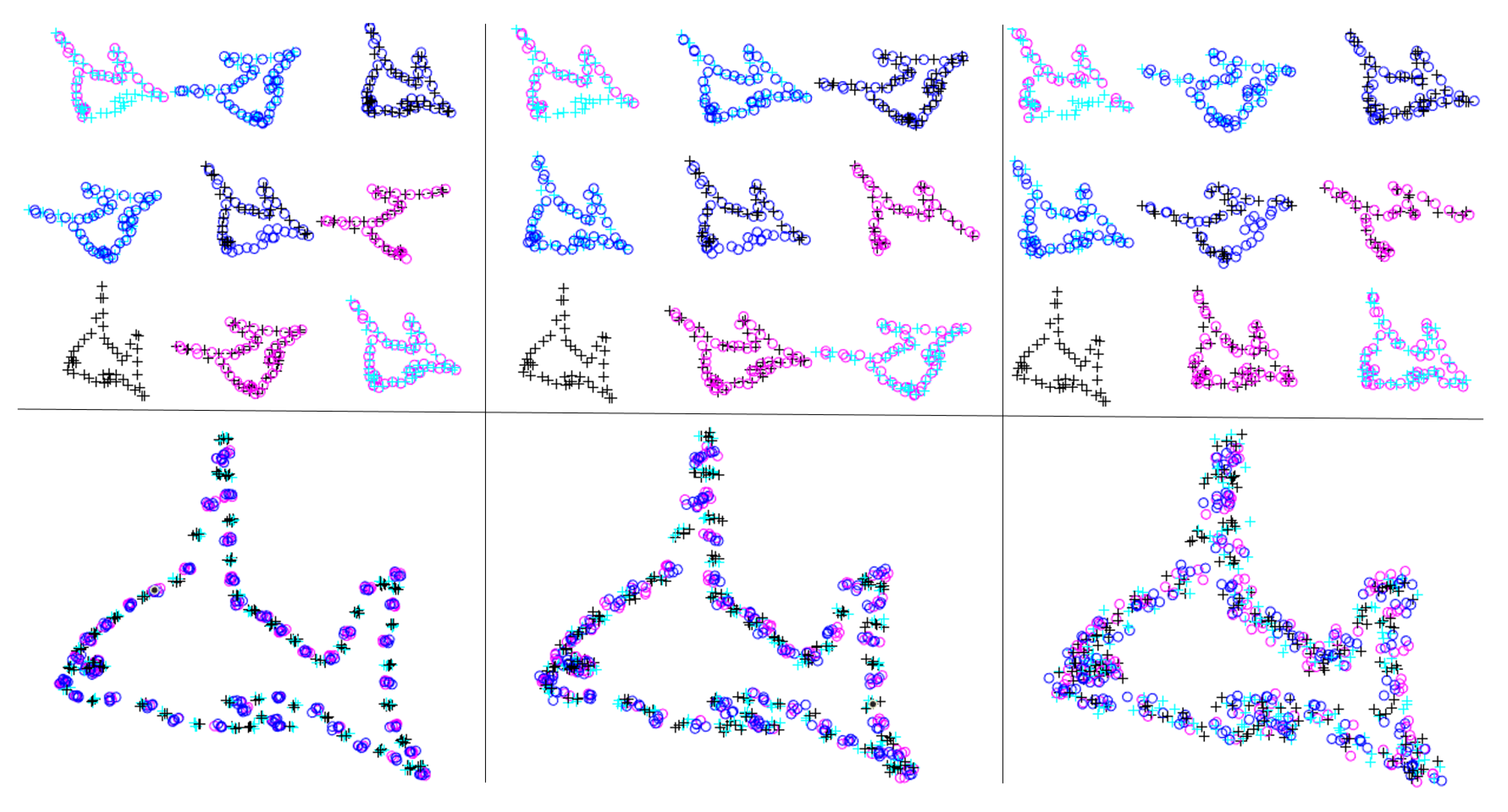
4.1. Robustness Test

As proved in Section 3.6, our algorithm obtains optimal solutions under ideal conditions. Therefore, we investigated whether our algorithm remains robust under nonideal circumstances (i.e., when the original accurate correspondence positions are randomly shifted by nonlinear deformation).
In this experiment, we used synthetic data to test the robustness. As shown in Figure 1, we sampled approximately 50 points from a fish-shaped point cloud to form 10 point sets. The first and last point sets overlap (at bottom left) to ensure that no relative displacement exists. The points with the same shape and color in adjacent point sets are corresponding points. To further verify generality, we sampled different numbers of points (as illustrated in the middle-right and top-left images). To prove that our algorithm is robust to noise, we added random deviations to each point; the different noise ratios are shown in Figure 1 and range from 0.05 to 0.2. We can see that as the noise ratio grows, the registered point cloud becomes progressively blurrier, but retains the overall fish shape.
To further demonstrate the generality of our algorithm, we investigated whether our algorithm was able to simultaneously align several point sets with small partial overlaps. As shown in Figure 2, unlike the first experiment, in which a complete fish shape was sampled, in this experiment, we sampled only a part of the fish at one time, resulting in eight point sets that partially overlap the adjacent point sets. Similar to the previous example, the correspondences are denoted by points with the same color and shape. The first and last point sets completely overlap; therefore, their relative positions do not need to be adjusted. We also added random noise proportional to the coordinates of each point to simulate real scenes. The experimental result is shown in the second row of Figure 2. These results show that, even when partial overlaps exist, our algorithm still achieves fine registration and is robust to noise.
To analyze the results quantitatively, we adopted the mean square error (MSE) to measure the accuracy between the ground truth of each example and our registration results. As Figure 3 shows, as the noise ratio increases, the MSE remains at a low level (below 0.06). Hence, we can conclude that our algorithm obtains accurate registration results even when inaccurate one-to-one correspondences are obtained.

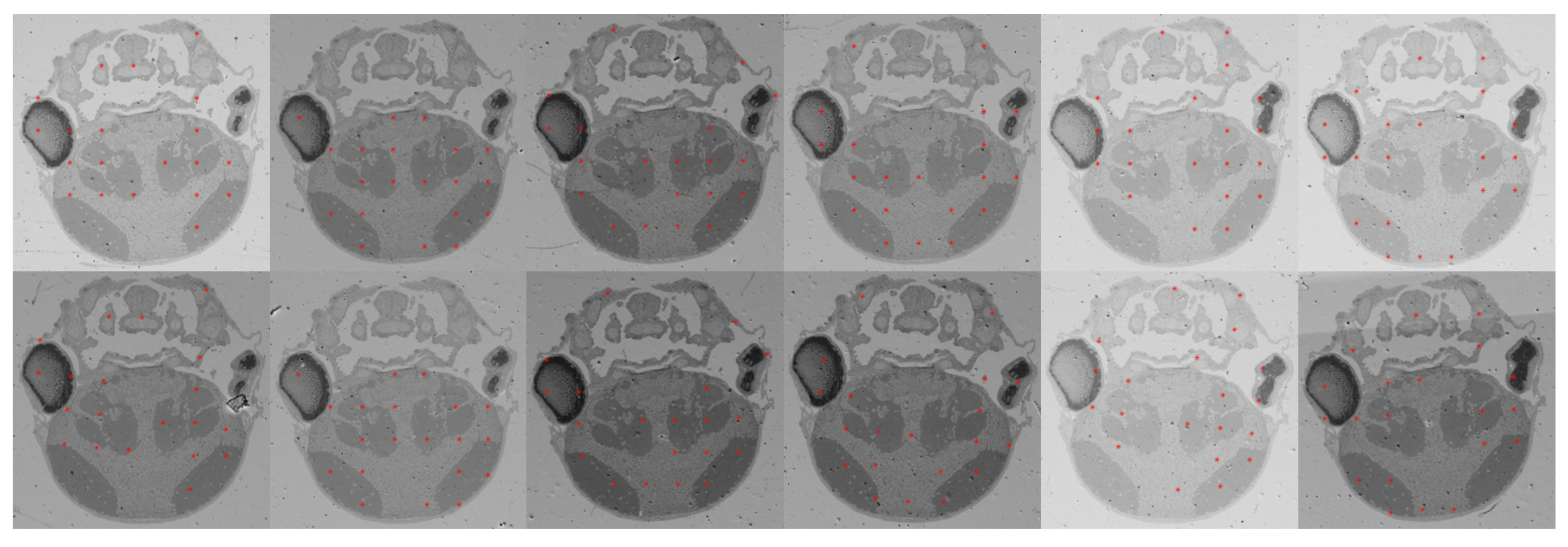
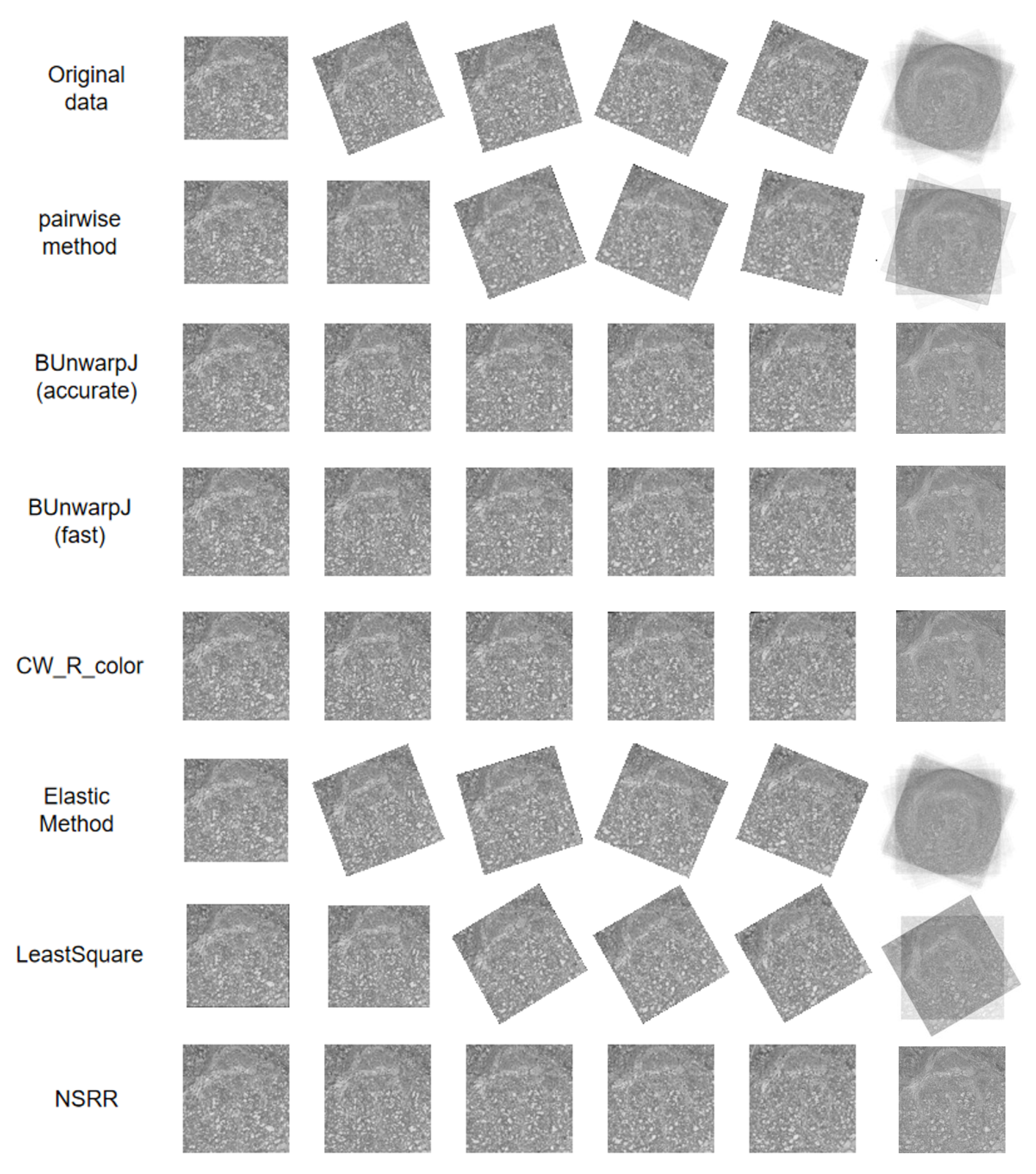
4.2. Comparison with State-of-the-Art Methods

To test the proposed algorithm’s applicability to real-world scenes, we first used our noniterative simultaneous rigid registration algorithm (NSRR) to register serial section images of a zebrafish, which included 336 microscopic images imaged by scanning electron microscopy (SEM). The thickness of each section is 50 nm, the image resolution is 6144 by 6144 pixels, and the pixel size of the images is 110 nm. This problem involves different levels of rotation, translation, scaling, and nonlinear deformation. All the experiments were run on the same PC equipped with an intel i7-4790 CPU. Baseline methods’ programs are publicly available in Fiji (the software can be downloaded from: https://imagej.net/Fiji and http://www-o.ntust.edu.tw/~cweiwang/3Dregistration/).
We utilized the SIFT flow method [20] to obtain dense correspondences, from which we selected a sparse set of correspondences with high confidence from the foreground, as illustrated in Figure 4.
The performance metric is SSIM [22], which evaluates the structural similarity between each pair of registered adjacent images; these values are summed and averaged across the entire sequence. Meanwhile, the SSIM variance along the whole sequence was calculated to evaluate the algorithms in terms of stability. We computed the total time needed to register an image pair to measure algorithm performance.
We adopted the widely used state-of-the-art methods described in Section 2 as baselines, including Pairwise method [23], BUnwarpJ [10], CW_R_color [3], LeastSquare [8], and Elastic method [12]. Here, Pairwise method was applied sequentially to register adjacent section images. Table 1 lists comparisons of the results among the baselines and our method. Compared with the baseline methods, our method achieves the highest accuracy in the least amount of time. Moreover, our method is very stable, and it achieves the smallest accuracy deviations. As Figure 5 shows, our method achieves the best results and does not cause error accumulation and propagation.
To further prove the effectiveness of our method, we also adopted the data acquired by FIB-SEM [24], which contains 62 serial section images of a Drosophila brain whose image resolution is 6684 × 6516 pixels with thicknesses and pixel sizes all equal to 9.15 nm. The advantage of using these data are that all the sections were imaged in situ; therefore, these data can be treated as the ground truth. It is well known that ground truth for image registrations is difficult to obtain; however, based on these data, we can construct a testing set that includes ground truth.
Each section was randomly rotated and shifted, and some sections were removed to mimic the common thicknesses of serial sections. Compared with the zebrafish SEM data, these data are considerably more complex, because the image content can be replete with many textures, the matching of fine details needs to be considered.
Similar to the last experiment, we compared the performance of our algorithm with all the baseline methods. We used endpoint error (EPE) to evaluate accuracy; EPE is the Euclidean distance between the registered images and the ground truth images, and it is averaged over all pixels. Here, an image is reshaped to a vector. Table 2 shows a comparison among the baseline methods and our method. Coinciding with the conclusion of the last experiment, our method achieves the least error in the least amount of time. Figure 6 shows a visualization of the registration results. As Figure 6 shows, our method achieves the best result and does not cause error accumulation and propagation. Moreover, it generates the clearest average image compared to the others. Some methods that previously obtained poor performances perform better on these data, such as BUnwarpJ and CW_R_color; however, the performance of our method remains stable.

5. Discussion

In this section, we discuss the applicability of our method. As we prove in Section 3.6, we must satisfy two conditions to obtain the optimal solution: first, all the serial sections must be rigidly deformed, and, second, the first and last images must have no relative displacement. For the first condition, since our algorithm is aimed at resolving rigid deformation, it it difficult to directly apply on nonrigidly distorted sections. However, our method can offer a good initial estimate for the nonrigid registration algorithms. For the second condition, we could image the top and bottom surfaces of the samples before sectioning, acquiring the images of the first and last sections. Since this step is conducted before sectioning, no relative displacement exists between the first and last sections.

6. Conclusions

This work presents and solves a constrained simultaneous rigid registration problem for serial section images. Because reliable correspondences can be extracted only from adjacent section images, the current 3D registration algorithms degenerate into processes that sequentially solve pairwise registration problems, resulting in error accumulation and propagation. To address this issue, we add the constraint that the positions of the first and last section images must remain unchanged; then, we estimate the optimal rigid transformations for the remaining section images to minimize the distances between their correspondences. The proposed method is noniterative and obtains the optimal solution under ideal conditions. It can simultaneously compute rigid transformations for large numbers of serial section images in a short time.

Author Contributions

This paper is a result of the full collaboration of all authors: conceptualization, C.S., X.C., and H.H.; data curation, L.-L.L. and G.L.; formal analysis, C.S. and X.C.; methodology, C.S. and X.C.; validation, C.S.; writing, C.S; and writing—review and editing, C.S., X.C. and H.H. All authors have read and agreed to the published version of the manuscript.

Funding

This research study was supported by the National Science Foundation of China (Nos. 61673381 and 61701497), Special Program of Beijing Municipal Science and Technology Commission (No. Z181100000118002), Strategic Priority Research Program of Chinese Academy of Science (No. XDB32030200), Instrument function development innovation program of Chinese Academy of Sciences (No. 282019000057), and Bureau of International Cooperation, CAS (No. 153D31KYSB20170059).

Conflicts of Interest

The authors declare no conflict of interest.

Appendix A. Proofs

Lemma A1.
The optimal solution of Equation (4) is W i = H i V i C i U i T , where U i S i V i T is the singular value decomposition (SVD) of A i , C i = d i a g ( 1 , det ( V i U i T ) ) , H i is 2 × 2 rotation matrix whose rotation degree θ i can be obtained by solving Equation (5), and θ is the rotation degree of i = 1 n V i C i U i T .
Proof of Lemma A1.
V i C i U i T is the optimal rotation matrix in pairwise point sets registration [23]. We can assume that W i = H i V i C i U i T , where H i is an unknown rotation matrix we need to evaluate. Using commutative law of multiplication for rotation matrix, the constraint in Equation (4) can be represented as
i = 1 n W i = i = 1 n V i C i U i T H i = i = 1 n V i C i U i T i = 1 n H i = I
Denoting the rotation degree of i = 1 n V i C i U i T to be θ and the rotation degree of H i to be θ i , we obtain i = 1 n θ i = θ . Using Lemma A2, the objective function in Equation (4) becomes:
i = 1 n 1 t r W i A i = i = 1 n 1 t r C i S i V i T H i V i = i = 1 n 1 t r C i S i cos ± θ i sin ± θ i sin ± θ i cos ± θ i = i = 1 n 1 t r C i S i cos θ i
Therefore, solving Equation (4) is equivalent to solving Equation (5). □
Lemma A2.
With orthogonal matrix O and rotation matrix P, we have O T PO = P or P T .
Proof of Lemma A2.
Since O is an orthogonal matrix, it is either a rotation matrix or a reflection matrix. If O is a rotation matrix, using the commutative law of multiplication for rotation matrix, O T PO = P O T O = P . If O is a reflection matrix, we denote Rot ( θ ) as a rotation matrix with rotation degree θ and Ref ( ϕ ) as a reflection matrix with reflection degree ϕ , that is
Rot ( θ ) = cos θ sin θ sin θ cos θ Ref ( ϕ ) = cos 2 θ sin 2 θ sin 2 θ cos 2 θ
It is known that:
Rot ( θ ) Ref ( ϕ ) = Ref ( ϕ + θ / 2 ) Ref ( θ ) Ref ( ϕ ) = Rot ( 2 ( θ ϕ ) )
Therefore,
O T PO = Ref ( ϕ ) Rot ( θ ) Ref ( ϕ ) = Rot ( θ ) = P T
 □

References

  1. Briggman, K.L.; Bock, D.D. Volume electron microscopy for neuronal circuit reconstruction. Curr. Opin. Neurobiol. 2012, 22, 154–161. [Google Scholar] [CrossRef] [PubMed] [Green Version]
  2. Helmstaedter, M. Cellular-resolution connectomics: Challenges of dense neural circuit reconstruction. Nat. Methods 2013, 10, 501–507. [Google Scholar] [CrossRef] [PubMed]
  3. Wang, C.W.; Gosno, E.B.; Li, Y.S. Fully automatic and robust 3D registration of serial-section microscopic images. Sci. Rep. 2015, 5, 15051. [Google Scholar] [CrossRef] [PubMed]
  4. Rossetti, B.J.; Wang, F.; Zhang, P.; Teodoro, G.; Brat, D.J.; Kong, J. Dynamic registration for gigapixel serial whole slide images. In Proceedings of the IEEE International Symposium on Biomedical Imaging, Melbourne, Australia, 18–21 April 2017; p. 424. [Google Scholar]
  5. Ourselin, S.; Roche, A.; Subsol, G.; Pennec, X.; Ayache, N. Reconstructing a 3D structure from serial histological sections. Image Vis. Comput. 2001, 19, 25–31. [Google Scholar] [CrossRef]
  6. Schmitt, O.; Modersitzki, J.; Heldmann, S.; Wirtz, S.; Fischer, B. Image registration of sectioned brains. Int. J. Comput. Vis. 2007, 73, 5–39. [Google Scholar] [CrossRef]
  7. Pichat, J.; Modat, M.; Yousry, T.; Ourselin, S. A multi-path approach to histology volume reconstruction. In Proceedings of the IEEE International Symposium on Biomedical Imaging, New York, NY, USA, 16–19 April 2015; pp. 1280–1283. [Google Scholar]
  8. Schindelin, J.; Arganda-Carreras, I.; Frise, E.; Kaynig, V.; Longair, M.; Pietzsch, T.; Preibisch, S.; Rueden, C.; Saalfeld, S.; Schmid, B.; et al. Fiji: An open-source platform for biological-image analysis. Nat. Methods 2012, 9, 676. [Google Scholar] [CrossRef] [PubMed] [Green Version]
  9. Lowe, D.G. Distinctive image features from scale-invariant keypoints. Int. J. Comput. Vis. 2004, 60, 91–110. [Google Scholar] [CrossRef]
  10. Arganda-Carreras, I.; Sorzano, C.O.; Marabini, R.; Carazo, J.M.; Ortiz-de Solorzano, C.; Kybic, J. Consistent and elastic registration of histological sections using vector-spline regularization. In Proceedings of the International Workshop on Computer Vision Approaches to Medical Image Analysis, Graz, Austria, 12 May 2006; pp. 85–95. [Google Scholar]
  11. Wang, C.W.; Ka, S.M.; Chen, A. Robust image registration of biological microscopic images. Sci. Rep. 2014, 4, 6050. [Google Scholar] [CrossRef] [PubMed] [Green Version]
  12. Saalfeld, S.; Fetter, R.; Cardona, A.; Tomancak, P. Elastic volume reconstruction from series of ultra-thin microscopy sections. Nat. Methods 2012, 9, 717–720. [Google Scholar] [CrossRef] [PubMed] [Green Version]
  13. Jaderberg, M.; Simonyan, K.; Zisserman, A. Spatial transformer networks. In Proceedings of the 28th International Conference on Neural Information Processing Systems, Montreal, QC, Canada, 7–12 December 2015; pp. 2017–2025. [Google Scholar]
  14. Shu, C.; Chen, X.; Xie, Q.; Han, H. An unsupervised network for fast microscopic image registration. In Proceedings of the Medical Imaging 2018: Digital Pathology, Houston, TX, USA, 10–15 February 2018; Volume 10581, p. 105811D. [Google Scholar]
  15. Yoo, I.; Hildebrand, D.G.; Tobin, W.F.; Lee, W.C.A.; Jeong, W.K. ssemnet: Serial-section electron microscopy image registration using a spatial transformer network with learned features. In Deep Learning in Medical Image Analysis and Multimodal Learning for Clinical Decision Support; Springer: Berlin/Heidelberg, Germany, 2017; pp. 249–257. [Google Scholar]
  16. Zhou, S.; Xiong, Z.; Chen, C.; Chen, X.; Liu, D.; Zhang, Y.; Zha, Z.J.; Wu, F. Fast and Accurate Electron Microscopy Image Registration with 3D Convolution. In Proceedings of the International Conference on Medical Image Computing and Computer-Assisted Intervention, Shenzhen, China, 13–17 October 2019; pp. 478–486. [Google Scholar]
  17. Dosovitskiy, A.; Fischer, P.; Ilg, E.; Hausser, P.; Hazirbas, C.; Golkov, V.; Van Der Smagt, P.; Cremers, D.; Brox, T. Flownet: Learning optical flow with convolutional networks. In Proceedings of the IEEE International Conference on Computer Vision, Santiago, Chile, 7–13 December 2015; pp. 2758–2766. [Google Scholar]
  18. Ilg, E.; Mayer, N.; Saikia, T.; Keuper, M.; Dosovitskiy, A.; Brox, T. Flownet 2.0: Evolution of optical flow estimation with deep networks. In Proceedings of the IEEE Conference on Computer Vision and Pattern Recognition, Honolulu, HI, USA, 21–26 July 2017; pp. 2462–2470. [Google Scholar]
  19. Sun, D.; Yang, X.; Liu, M.Y.; Kautz, J. PWC-net: CNNs for optical flow using pyramid, warping, and cost volume. In Proceedings of the IEEE Conference on Computer Vision and Pattern Recognition, Salt Lake City, UT, USA, 18–23 June 2018; pp. 8934–8943. [Google Scholar]
  20. Liu, C.; Yuen, J.; Torralba, A. Sift flow: Dense correspondence across scenes and its applications. IEEE Trans. Pattern Anal. Mach. Intell. 2011, 33, 978–994. [Google Scholar] [CrossRef] [PubMed] [Green Version]
  21. Hager, W.W. Updating the Inverse of a Matrix. Siam Rev. 1989, 31, 221–239. [Google Scholar] [CrossRef]
  22. Wang, Z.; Bovik, A.C.; Sheikh, H.R.; Simoncelli, E.P. Image quality assessment: From error visibility to structural similarity. IEEE Trans. Image Process. 2004, 13, 600–612. [Google Scholar] [CrossRef] [PubMed] [Green Version]
  23. Arun, K.S.; Huang, T.S.; Blostein, S.D. Least-Squares Fitting of Two 3-D Point Sets. IEEE Trans. Pattern Anal. Mach. Intell. 1987, 9, 698. [Google Scholar] [CrossRef] [PubMed] [Green Version]
  24. Knott, G.; Marchman, H.; Wall, D.; Lich, B. Serial section scanning electron microscopy of adult brain tissue using focused ion beam milling. J. Neurosci. 2008, 28, 2959–2964. [Google Scholar] [CrossRef] [PubMed]
Figure 1. Experimental results. Ten point sets with different degrees of noise ratios from 0.05 to 0.2 are shown from left to right in the first row. The corresponding registration results by our algorithm are shown in the second row.
Applsci 10 01156 g001
Figure 2. Experimental results. Eight point sets with different degrees of noise ratios from 0.05 to 0.2 are shown from left to right in the first row. The corresponding registration results by our algorithm are shown in the second row.
Applsci 10 01156 g002
Figure 3. Plot of MSE versus noise ratio.
Applsci 10 01156 g003
Figure 4. An example of the correspondences we extracted (marked by red dots). We utilized the SIFT flow method to obtain dense correspondences between adjacent images; then, from those, we selected a sparse set of pairs with low matching errors. The two rows show adjacent images. Clearly, our approach can obtain reliable correspondences even under conditions that involve illumination variation, tissue removal, and spatial transformation.
Applsci 10 01156 g004
Figure 5. An example of our experimental results on the zebrafish SEM data. To provide a clear demonstration of the registration effects, we averaged the registered sequence and show the results in the last column.
Applsci 10 01156 g005
Figure 6. An example of our experimental results on the Drosophila brain FIB-SEM data. The original data contain large rigid deformations, and most methods tend to cause error accumulation and propagation. To provide a clearer demonstration of the registration effects, we averaged the registered sequence and show the results in the last column.
Applsci 10 01156 g006
Table 1. Comparison of accuracy and speed in Zebrafish SEM data.
MethodSSIMTime
BUnwarpJ(fast) [10]0.6523 ± 0.12353.6 min
BUnwarpJ(accurate) [10]0.7037 ± 1.27174.3 min
LeastSquare [8]0.8046 ± 0.157811.729 s
Elastic Method [12]0.6118 ± 0.09681.4 min
CW_R_color [3]0.6721 ± 0.901336.4 min
Pairwise method [23]0.7331 ± 0.12830.937 s
NSRR (ours)0.8297 ± 0.07060.2813 s
Table 2. Comparison of accuracy and speed in Drosophila brain FIB-SEM data.
MethodEPETime
BUnwarpJ(fast) [10]16.62433.4 min
BUnwarpJ(accurate) [10]14.31405.5 min
LeastSquare [8]15.40135.462 s
Elastic Method [12]17.614110.323 s
CW_R_color [3]12.77548.1 min
Pairwise method [23]14.52770.368 s
NSRR (ours)11.19030.289 s

