An Assemble Based on Clustering and Monte Carlo for the Wavelengths Selection of Excitation Emission Fluorescence Spectra

Abstract

Excitation-emission fluorescence spectra is very effective to predict the concentration of organics in samples. However, redundant information and noises in the excitation-emission matrix (EEM) decrease the accuracy of the prediction concentration. Here we proposed a method to select more useful excitation and emission spectra from the EEM to increase the accuracy of prediction concentration and reduce the processing time. First, the excitation wavelengths were selected based on the clustering method to limit the redundant information in the EEM. Then the emission wavelengths were selected based on the Monte-Carlo method. To validate this method, we established the concentration prediction model with the spectra corresponding to the selected wavelengths by partial least square regression and predicted the multi component concentrations in the test samples. Our studies indicate that incorporation of this method increases the accuracy of the prediction concentration of organics and reduces the processing time.

1. Introduction

Spectrofluorimetry has been widely implemented to predict the concentration of organics in samples for its advantages of sensitivity, selectivity, non-invasiveness, and fastness [1,2]. To date, the emission fluorescence spectrum, which is excited by single excitation wavelength, is commonly used to predict the concentration of organics. Alternatively, an excitation-emission matrix (EEM) of the sample acquired by choosing individual excitation wavelengths is better to analyze the organics quantitatively, which consists of multiple emission spectra and includes more information of the samples. However, some of these emission fluorescence spectra are linearly correlated, by which lead to extra redundant information [3,4], and Rayleigh scattering of the light also contributes to the EEM, which is known as noises. All this subordinate information is infaust for predicting the concentration of the organics [5]. To increase the accuracy of concentration prediction, the excitation and emission wavelengths in the EEM should be selected.

To date most reported researches are focused on the selection of the emission wavelengths from the emission spectrum. The methods, for example, partial least squares regression (PLSR), moving window PLS, iterative predictor weighting-PLS, and uninformative variable elimination-PLS [6,7,8,9,10,11], establish multi concentration prediction models with every emission wavelength in turn and the wavelengths corresponding to the lowest prediction concentration error are finally reserved. Comparing to these methods, the genetic algorithm (GA) and Monte Carlo method have more wavelengths selection throughput [12,13,14,15], because emission wavelengths are selected by taking into account their contribution to the concentration prediction. The initial contribution to the concentration of each wavelength is presumably the same for GA, which is not consistent with the actuality; and the predetermined criteria is given for Monte Carlo to reserve the emission wavelengths which contribute most to the concentration. Considering the linear correlation between emission spectra excited by different wavelengths, all emission spectra are categorized into different classes based on their similarity, by aligning the similarity coefficients between different emission spectra in each class. Only the emission spectrum with the maximal similarity coefficient between it and the other emission spectra is reserved to eliminate the influence of the redundant information between different emission spectra.

Overall, we developed a method to increase the accuracy of the prediction concentration based on the EEM, by which the excitation wavelengths and the emission wavelengths are selected respectively. This approach involves three discrete steps: (a) The clustering method is performed to categorize the emission spectra into different classes, only the emission spectrum with the maximal similarity coefficient between it and the other emission spectra in each class is reserved; then (b) all the reserved emission spectra are unfolded to one dimension emission spectrum by sorting their corresponding excitation wavelengths in ascending order, and the Monte Carlo method combined with PLSR is applied to refine the emission wavelengths; and finally (c) the prediction concentration model is established by the spectra corresponding to the selected wavelengths.

2. Methods

2.1. Selection of the Excitation Wavelengths by the Clustering Method

The typical EEM is described in

Table 1. The excitation-emission matrix (EEM).

	Ex1	…	Exj	…	ExJ
Em1	X11	…	Xj1	…	XJ1
⋮	⋮	⋮	⋮	⋮	⋮
Emi	X1i	…	Xji	…	XJi
⋮	⋮	⋮	⋮	⋮	⋮
EmI	X1I	…	XjI	…	XJI

. E_x1, …, E_xj, …, E_xJ are the J excitation wavelengths, E_m1, …, E_mi, …, E_mI are the I emission wavelengths, and X_ij is the fluorescence intensity corresponding to the i^th emission wavelength excited by the j^th wavelength. Let (X_a1, X_a2, …, X_aI)^T and (X_b1, X_b2, …, X_bI)^T be the emission intensity spectra relating to the a^th and the b^th excitation wavelengths, respectively. The similarity coefficient $C_{ab}$ between these two emission spectra is calculated by Equation (1), as follows:

$$C_{ab}=\frac{{\displaystyle \sum _{i=1}^I(X_{ai}-{\overline{X}}_a)}(X_{bi}-{\overline{X}}_b)}{\sqrt{{\displaystyle \sum _{i=1}^I{(X_{ai}-{\overline{X}}_a)}^2{\displaystyle \sum _{i=1}^I{(X_{bi}-{\overline{X}}_b)}^2}}}}$$

(1)

where ${\overline{X}}_a,{\overline{X}}_b$ are the mean fluorescence intensity of the a^th and the b^th emission spectra, respectively.

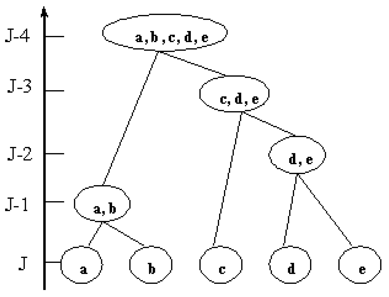
Initially there are J excitation wavelength classes (Figure 1), corresponding to J excitation wavelengths, then the similarity coefficients between any two emission spectra corresponding to their excitation wavelengths are calculated, after the pair of emission spectra with the largest similarity coefficient are designated as one class, J-1 excitation wavelength classes are left. The number of classes is reduced by one after each calculation round of the similarity coefficient. This process is performed until the difference of similarity coefficients between any two pair of classes are under the pre-defined tolerant criterion.

When two or more excitation wavelengths are assigned to the same class, the calculation of the similarity coefficient between different classes is different from that between each single emission spectrum. Let M and N be two different classes with m and n emission spectra in each class, the similarity coefficient calculation steps are: First, the similarity coefficients between one emission spectrum in class M and the n emission spectra in class N are calculated; then another emission spectrum in class M is assigned to repeat the above step. Once all $m\times n$ similarity coefficients are calculated, the two excitation wavelengths corresponding to the maximum similarity coefficient between the class M and N are accepted to represent each class.

The EEM of pure organic compound sample is used to select its excitation wavelengths. The spectra corresponding to these wavelengths will be served to select the emission wavelengths.

2.2. Selection of the Emission Wavelengths by the Monte Carlo Method

The P training samples with known concentrations of each component are used to establish the prediction concentration model. Presumably k excitation wavelengths are retained for each component by the method given in Section 2.1, the k emission spectra corresponding to specific excitation wavelengths are unfolded into a one-dimensional emission spectrum in the ascending order of the excitation wavelengths, that is,

$$X={(X_{11},\dots ,X_{i1},\dots ,X_{I1},X_{12},\dots ,X_{i2},\dots ,X_{I2},\dots ,X_{1k},\dots ,X_{ik},\dots ,X_{Ik})}^T$$

(2)

Each sample has I emission wavelengths, leading to a total of I × k emission wavelengths. There are P unfolding emission spectra for P training samples.

The Monte Carlo method combined with PLSR is applied to select the emission wavelengths from P unfolding emission spectra as Formula (2). For each iteration, l emission wavelengths are randomly picked out from each X, a l × P sub-emission matrix X_l is formed with P unfolding spectra. The prediction concentration model is constructed with X_l based on PLSR [10,11]. The root mean square error of correction (RMSEC) is calculated by Equation (3):

$$RMSEC=\sqrt{\frac{{\displaystyle \sum _{c=1}^C{({\tilde{y}}_c-y_c)}^2}}{C}}$$

(3)

where y_c is the known concentration of component c, ${\tilde{y}}_c$ is the predicted concentration of c, and C is the number of components. The reliability of the prediction for each iteration is calculated by d_j = 1/RMSEC.

After 20,000 iterations of above step, if the i^th emission wavelength is selected Q times, the reliability score S_i of the i^th emission wavelength is summed by

$$Si=\frac{1}{Q}{\displaystyle \sum _{j=1}^Q{d}_j}$$

(4)

The reliability scores of the I × k emission wavelengths are calculated and the top 10% emission wavelengths are reserved. These selected emission wavelengths will be used to predict concentrations in the test samples.

3. Experimental Method and Results

3.1. Apparatus and Sample Preparation

Three organic compounds used for this study were naphthalene, 1-naphthol, and 2-naphthol. The samples of the three pure compounds were mixed into another 11 samples of different concentrations. We used the training set (nine samples) to establish the prediction concentration model, and the test set (two samples) to validate the accuracy of the concentration prediction.

Table 2. Concentrations of components in samples (mg/L).

Sample		Naphthalene	1-Naphthol	2-Naphthol
Test samples #	1	0.2500	0.2500	0.2000
	2	0.2700	0.4000	0.3000
Training samples #	1	0.1000	0.1000	0.1000
	2	0.1000	0.2000	0.4000
	3	0.1000	0.5000	0.5000
	4	0.3000	0.1000	0.4000
	5	0.3000	0.2000	0.5000
	6	0.3000	0.5000	0.1000
	7	0.5000	0.1000	0.5000
	8	0.5000	0.2000	0.1000
	9	0.5000	0.5000	0.4000

listed the components concentrations of all samples. Besides, eleven blank samples were also prepared without the above three organics compounds.

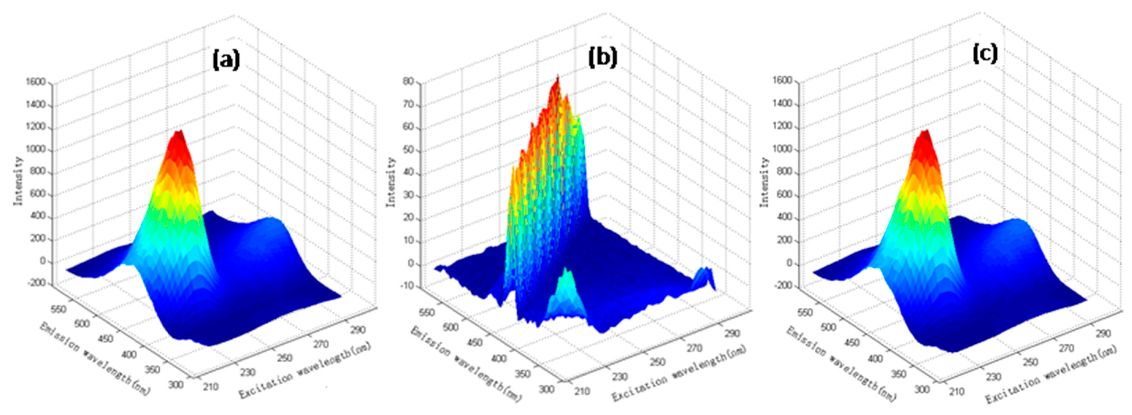
The EEMs of the three pure compounds, the nine training samples, the two test samples, and eleven blank samples were collected over excitation wavelengths between 220 and 300 nm with a 2 nm interval and over emission wavelengths between 325 and 600 nm with a 5 nm interval by a Hitachi F-7000 spectrofluorometer at room temperature of 25 °C. The EEM of each sample was subtracted by the mean EEM of the eleven blank samples to eliminate the influence of the background noises. As an example, Figure 2 shows the original EEM of naphthalene, the mean EEM of the blank samples, and the blank-subtracted naphthalene.

3.2. Results of the Selected Wavelengths

The clustering method was used to select the excitation wavelengths for each pure compound with the pure compound EEM. The tolerant criterion was set to 1.3 × 10⁻³.

Table 3. The selected excitation wavelengths for the pure compound (nm).

Name of the Pure Compound	Selected Excitation Wavelengths
naphthalene	220	224	230	234	236	252	254	262	270	272
1-naphthol	222	230	248	250	252	256	258	260	290	292
2-naphthol	248	250	252	254	260	262	266	268	278	288

gives the 10 selected excitation wavelengths of each component from 41 excitation wavelengths. The selected excitation wavelengths of each component are different, which can presume it relates to their specific molecular structures.

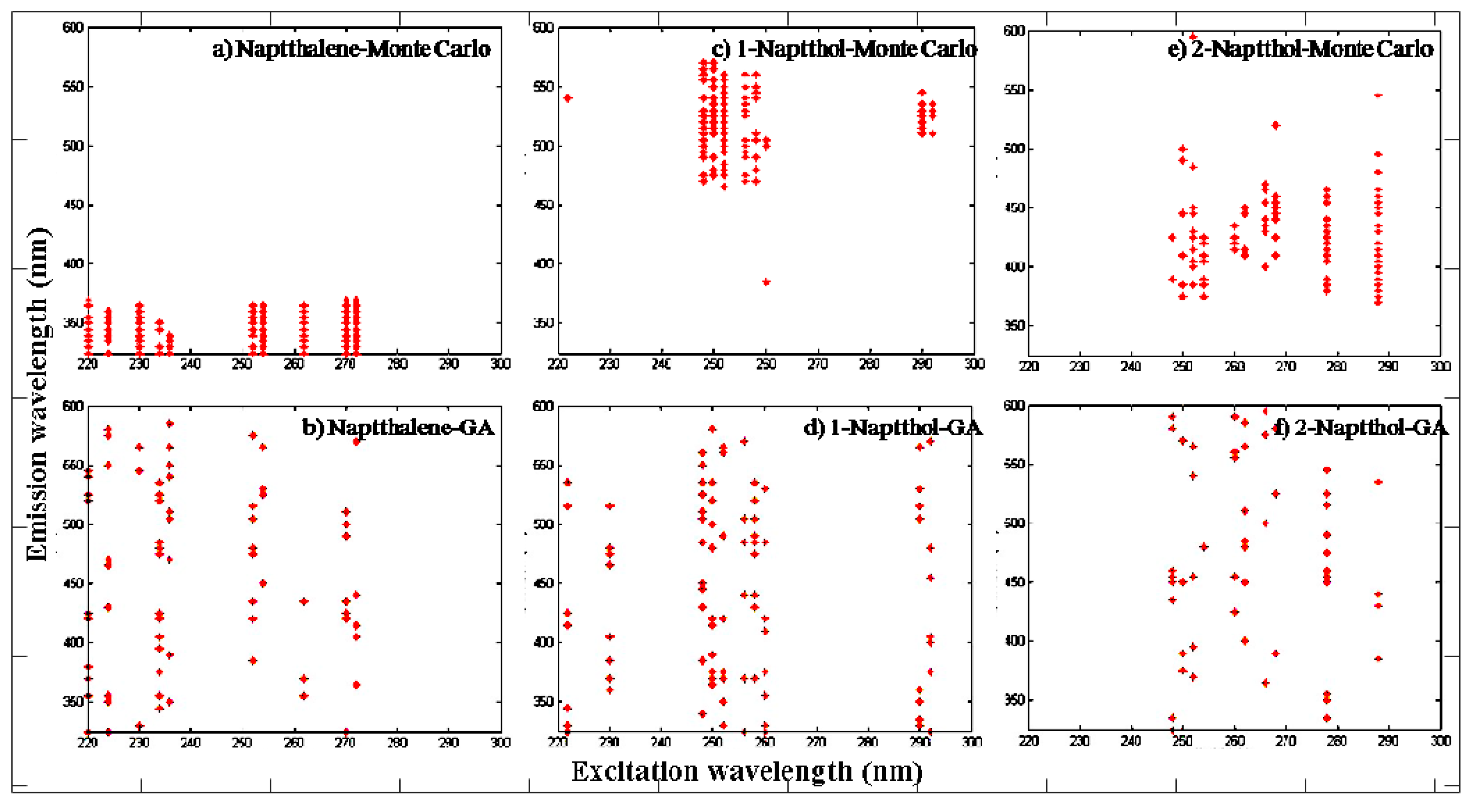
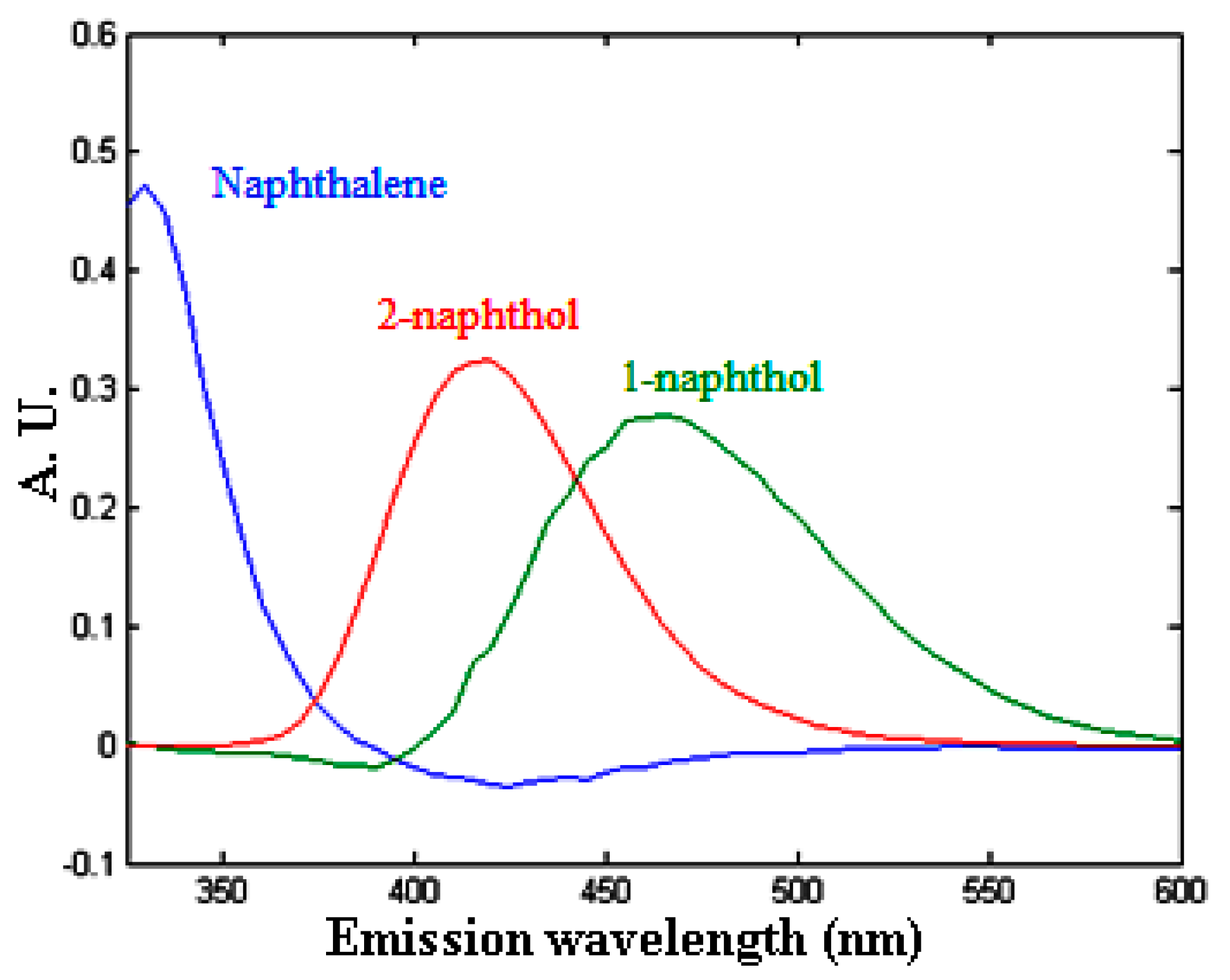
We used the emission spectra corresponding to the 10 selected excitation wavelengths of the nine training samples to find the emission wavelengths based on the method given in Section 2.2. The dots in Figure 3a,c,e are the selected emission wavelengths, which are 63 for naphthalene, 64 for 1-naphthol, and 71 for 2-naphthol. These emission wavelengths fell within the emission spectra peak band of each compound excited by specific wavelength, as plotted in Figure 4. For comparison, we used the same emission spectra corresponding to the selected excitation wavelengths to select the emission wavelengths by the GA method, as shown in Figure 3b,d,f. As it can be seen in Figure 3b,d,f, these wavelengths extended across the entire band of the emission wavelengths. The Monte Carlo method in this study is more effective than the GA method presumably that the emission wavelengths within the peak band contribute most to the concentration prediction.

3.3. Results of Concentration Prediction

The predicted concentration models were established with all spectra of the training samples and the spectra corresponding to the selected wavelengths based on our proposed method of the training samples by the PLSR to predict the concentrations of the test samples.

Table 4. Predicted concentrations of the three components in the test samples.

Wavelength	Components		Naphthalene	1-Naphthol	2-Naphthol
Full wavelength predication	Sample 1 (mg/L)	actual concentration	0.2500	0.2500	0.2000
		predication concentration(mg/L)	0.2329	0.2621	0.2150
	Sample 2 (mg/L)	actual concentration	0.2700	0.4000	0.3000
		predication concentration(mg/L)	0.2840	0.4086	0.3173
	run time (s)		356.37	405.86	382.53
	RMSEP (%)		2.89	1.77	1.78
Selected wavelength predication	Sample 1 (mg/L)	actual concentration	0.2500	0.2500	0.2000
		predication concentration(mg/L)	0.2260	0.2445	0.1889
	Sample 2 (mg/L)	actual concentration	0.2700	0.4000	0.3000
		predication concentration(mg/L)	0.2619	0.4065	0.2954
	run time (s)		127.67	130.98	127.26
	RMSEP (%)		1.35	1.05	1.62

RMSEP: the root mean squared error of prediction concentration.

gives the root mean squared error of prediction concentration (RMSEP) with these two different spectra to assess the accuracy of the predicted concentrations. As can be seen, the RMSEP for Naphthalene, 1-naphthol, and 2-naphthol with the selected wavelengths are 1.35%, 1.05%, and 1.62%, respectively. However, the RMSEP for Naphthalene, 1-naphthol, and 2-naphthol with the full wavelengths are 2.89%, 1.77%, and 1.78%, respectively. The RMSEP for three compounds with the selected wavelengths are all lower than those with all wavelengths. The running time for the concentration prediction with all wavelengths and the selected wavelengths is also given in Table 4. The running time for Naphthalene, 1-naphthol, and 2-naphthol with the selected wavelengths is 127.67, 130.98, and 127.26 s, respectively. However, the running time for Naphthalene, 1-naphthol, and 2-naphthol with the full wavelengths is 356.37, 405.86, and 382.53 s, respectively. It is also obvious that the running time with the selected wavelengths is shorter than that with all wavelengths.

4. Conclusions

This study aims to increase the accuracy of the prediction concentration by selecting the excitation wavelengths and emission wavelengths from the EEM. To eliminate the redundant information, the excitation wavelengths were selected based on the clustering method; to refine the most useful emission wavelengths, the emission wavelengths corresponding to the selected excitation wavelengths were determined based on the Monte Carlo method. Comparing to the predicted concentration with all spectra, the accuracy of the prediction concentrations with the selected spectra is increased by selecting the irrelevant excitation spectra and reserving the emission wavelengths contributing most to predict component concentration based on the proposed method. The RMSEP for Naphthalene, 1-naphthol, and 2-naphthol with the selected wavelengths are 1.54%, 0.72%, and 0.16% lower than those with all wavelengths, respectively. Furthermore, the running time of the concentration prediction is also reduced because only the selected spectra were used instead of the full spectra. The running time for Naphthalene, 1-naphthol, and 2-naphthol with the selected wavelengths is 228.7, 274.88, and 255.27 s shorter than that with all wavelengths, respectively.

References

- Henderson, R.K.; Baker, A.; Murphy, K.R. Fluorescence as a potential monitoring tool for recycled water systems: A review. Water Res. 2009, 43, 863–881. [Google Scholar] [CrossRef] [PubMed]
- Zhigang, W.; Wenqing, L.; Yujun, Z.; Hongbin, L.I.; Nanjing, Z.; Jianguo, L.; Weichang, S.M.; Lishu, Y. Comparative research on determination of water integrated organic pollution index with three dimensional excitation-emission fluorescence spectroscopy and traditional wet chemical methods. Spectrosc. Spectr. Anal. 2007, 27, 2514–2517. [Google Scholar]
- Dan, J.; Yujun, Z.; Guogang, L. Three dimensional fluorescence spectra analysis of four kinds of polycyclic aromatic hydrocarbons. J. Atmos. Environ. Opt. 2008, 3, 448–453. [Google Scholar]
- Baghoth, S.A.; Sharma, S.K.; Amy, G.L. Tracking natural organic matter (NOM) in a drinking water treatment plant using fluorescence excitation-emission matrices and PARAFAC. Water Res. 2008, 20, 797–809. [Google Scholar] [CrossRef] [PubMed]
- Jing, L.; Liping, S.; Weiwei, Q.; Hu, D.; Jie, W. Study of redundant information in flouroscence spectra data analysis. Spectrosc. Spectr. Anal. 2010, 30, 2685–2688. [Google Scholar]
- Cramer, J.A.; Kramer, K.E.; Johnson, K.J.; Morris, R.E.; Rose-Pehrsson, S.L. Automated wavelength selection for spectroscopic fuel models by symmetrically contracting repeated unmoving window partial least squares. Chemom. Intell. Lab. Syst. 2008, 92, 13–21. [Google Scholar] [CrossRef]
- Vallade, J.; Stéphane, T.; Laroche, G. Partial least squares regression as a tool to predict fluoropolymer surface modification by dielectric barrier discharge in a corona process configuration in a nitrogen-organic gaseous precursor environment. Ind. Eng. Chem. Res. 2018, 57, 7476–7485. [Google Scholar] [CrossRef]
- Kaneko, H.; Muteki, K.; Funatsu, K. Improvement of iterative optimization technology (for process analytical technology calibration-free/minimum approach) with dimensionality reduction and wavelength selection of spectra. Chemom. Intell. Lab. Syst. 2015, 147, 175–184. [Google Scholar] [CrossRef]
- Jiang, J.H.; Berry, R.J.; Siesler, H.W.; Ozaki, Y. Wavelength interval selection in multi component spectral analysis by moving window partial least-squares regression with applications to mid-infrared and near-infrared spectroscopic data. Anal. Chem. 2002, 74, 3555–3565. [Google Scholar] [CrossRef] [PubMed]
- Matías, I.; Carlos, R.; Marcelo, F.P.; Beatriz, S.F.B. Simultaneous determination of quality parameters in biodiesel/diesel blends using synchronous fluorescence and multi variate analysis. Microchem. J. 2013, 108, 32–37. [Google Scholar]
- Bro, R.; Asmund, R.; Fabe, N.M. Standard error of prediction for multilinear PLS. practical implementation in fluorescence spectroscopy. Chemom. Intell. Lab. Syst. 2005, 75, 69–76. [Google Scholar]
- Héctor, C.G.; Olivieri, A.C. Wavelength selection for multivariate calibration using a genetic algorithm: A novel initialization strategy. J. Chem. Inf. Comput. Sci. 2002, 42, 1146–1153. [Google Scholar]
- Liguo, W.; Fangjie, W. Band selection for hyperspectral imagery based on combination of genetic algorithm and ant colony algorithm. J. Image Graph. 2013, 2, 235–242. [Google Scholar]
- Mingjian, H.; Quan, W.; Zhiyu, W. New near infrared wavelength selection algorithm based on Monte-Carlo Method. Acta Opt. Sin. 2010, 30, 3637–3642. [Google Scholar] [CrossRef]
- Han, Q.J.; Wu, H.L.; Cai, C.B.; Xu, L.; Yu, R.Q. An ensemble of Monte Carlo uninformative variable elimination for wavelength selection. Anal. Chem. Acta 2008, 6, 121–125. [Google Scholar] [CrossRef] [PubMed]
© 2020 by the authors. Licensee MDPI, Basel, Switzerland. This article is an open access article distributed under the terms and conditions of the Creative Commons Attribution (CC BY) license (http://creativecommons.org/licenses/by/4.0/).