Article

Whole-Body Dynamic Analysis of Challenging Slackline Jumping

Optimization, Robotics and Biomechanics (ORB), Institute of Computer Engineering (ZITI), Heidelberg University, 69117 Heidelberg, Germany
*
Author to whom correspondence should be addressed.
Appl. Sci. 2020, 10(3), 1094; https://doi.org/10.3390/app10031094
Submission received: 31 December 2019 / Revised: 29 January 2020 / Accepted: 1 February 2020 / Published: 6 February 2020
(This article belongs to the Special Issue Biomechanical Spectrum of Human Sport Performance)

Abstract

:
Maintaining balance on a slackline is a challenging task in itself. Walking on a high line, jumping and performing twists or somersaults seems nearly impossible. Contact forces are essential to understanding how humans maintain balance in such challenging situations, but they cannot always be measured directly. Therefore, we propose a contact model for slackline balancing that includes the interaction forces and torques as well as the position of the Center of Pressure. We apply this model within an optimization framework to perform a fully dynamic motion reconstruction of a jump with a rotation of approximately 180 ° . Newton’s equations of motions are implemented as constraints to the optimization, hence the optimized motion is physically feasible. We show that a conventional kinematic analysis results in dynamic inconsistencies. The advantage of our method becomes apparent during the flight phase of the motion and when comparing the center of mass and angular momentum dynamics. With our motion reconstruction method all momentum is conserved, whereas the conventional analysis shows momentum changes of up to 30%. Furthermore, we get additional and reliable information on the interaction forces and the joint torque that allow us to further analyze slackline balancing strategies.

1. Introduction

Slackline balancing is a recreational sport where the athlete tries to stand, walk or jump on a spring-like elastic ribbon band that is mounted between two anchor points as shown in Figure 1. Unlike balancing on a stiff beam or when performing a tandem walk on a regular surface, the slackline can swing both sideways and vertically, which increases the difficulty of maintaining an upright position [1]. In ongoing work, we investigate how humans maintain balance on a slackline and, to date, motion captured over 20 subjects of different skill levels. This led to a big data set containing standing, walking and jumping motions from beginners, intermediate and expert subjects. We previously analyzed different performance indicators for standing and walking based on kinematic measurements and subject-specific rigid body modeling [2] and found that experts show reduced angular momentum around the vertical axis and reduced Center of Mass (CoM) acceleration due to adjusted stance leg compliance. The analysis, however, lacks information on the interaction forces with the slackline. They are fundamental for understanding human locomotion [3] and would allow us to further investigate the data. The measurement of Ground Reaction Forces (GRF) enables us to compute joint torques, assess stability parameters in balancing tasks and is therefore part of many gait analysis protocols [4,5]. Pressure sensors and insoles are undergoing rapid development and are applied in various setups to measure interaction forces [6], however, it is not always possible to measure all forces directly for every task. Slackline balancing is usually done barefoot as experts report higher contact friction with the slackline which is crucial when landing from jumping. Beginners also prefer barefoot balancing over wearing shoes because they get a better feedback and control of the contact force. In the literature there are no reports on instrumented slacklines that can measure all interaction forces between the slackline and the subject. Previous work by Karatsidis et al. [7] estimated GRF for walking based only on inertial measurement data, a dynamic subject model and a heuristic on how the GRF are distributed during the double support phase. In previous work, we applied optimization methods and rigid body modeling to reconstruct GRF from kinematic data for sprinting motions with prostheses [8] and for a gymnastic cartwheel motion [9]. A dynamic model of the subject and a specific model of the interaction was crucial to obtain meaningful results. We now propose a new contact model specifically for balancing on a slackline and demonstrate its application by formulating and solving an optimal control problem (OCP) that reconstructs joint torques and forces of the slackline from marker-based motion capture and purely kinematic data. Newton’s equations of motions are implemented as constraints to the optimization and therefore the optimized motion is physically feasible. When analyzing jumping motions with the conventional kinematic method we found inconsistencies in the CoM and angular momentum dynamics during the flight phase. In this work, we show the advantage of the proposed analysis for a jump motion with rotation as an example.

2. Materials and Methods

2.1. Experimental Approach to the Problem

We present an overview of the slackline measurements and the data acquisition in Section 2.2. The conventional way of analyzing the data is described in Section 2.3. In a pre-study we investigated the differences between a regular planar contact and the contact with the slackline using sensor insoles (Section 2.4). The new analysis method is described in Section 2.5. It is based on the new contact model (Section 2.5.1) that takes the contact force, the contact torque and the position of the Center of Pressure (CoP) position into account. The subject-specific modeling and the formulation of the rigid body system dynamics with external contact forces are described in Section 2.5.2. In Section 2.5.3 we formulate and solve an OCP that tracks the recorded kinematic data by employing the proposed model. As  a result we obtain a fully dynamic description of the motion, including joint torques and contact  forces. We apply our approach to reconstruct the dynamics of one example motion where the subject jumps on the slackline and performs a rotation of approximately 180 ° . A visualization of the resulting motion and the contact forces and torques is shown in Section 3. We validate the OCP result by computing the CoM and angular momentum dynamics to show that the motion is physically feasible and follows Newton’s mechanics (Section 2.5.4). We then compare the proposed method to the results of a conventional analysis that is often used in the literature.

2.2. Slackline Study and Data Acquisition

The slackline was installed using the Gibbon Slackrack 300 (ID Sports GmbH, Gibbon Slacklines, Stuttgart, Germany) as shown in Figure 1. The slackline was 3 m in length, 5 cm in width and mounted 31 cm above the ground. The motions were recorded using the marker-based motion capture system Qualisys (Qualisys, Goeteborg, Sweden) consisting of 8 Oqus 500 cameras at a frame rate of 150 Hz. The subject was prepared with 49 spherical infrared-reflective markers of 14 mm diameter, following the bone landmarks of the Gait-IOR marker set [10]. This marker set has originally been designed for gait analysis and was extended by two additional markers on the Medial Epicondyle of the Humerus to allow for better upper arm tracking and shoulder angle reconstruction. A static pose was recorded to create the subject-specific rigid body model. Six static markers were removed after this pose following the Gait-IOR guidelines, since the static markers were located at the medial side of the leg segments and are often occluded, thus tending to collide with other body parts and eventually hinder free movement. All dynamic motions were recorded using the remaining 45 markers. The slackline motion capture experiments were approved by the ethics committee of the Faculty of Behavioral and Cultural Studies of Heidelberg University according to the Helsinki Declaration (AZ Mom 2016 1/2-A1, 2016 with amendment 2019). Written informed consent was obtained from the subject. before the measurements. The subject was 1.9 m tall, weight 86 kg and was 27 years old and had considerable experience in slackline balancing.

2.3. Conventional Analysis

In conventional motion analysis the joint angles of the rigid body model are computed using whole-body inverse kinematics for every frame individually. We used the open source sofware tool Puppeteer by Martin Felis [11] for this task. It employs a damped Levenberg-Marquardt algorithm, described by Sugihara [12], to solve for the whole-body posture on a frame-by-frame basis. Afterwards, a low-pass filter was applied to generate smooth and differentiable joint trajectories. Joint velocities and joint accelerations are computed using finite central differences. The resulting trajectories represent the measured kinematics and we can compute different mechanical properties such as CoM acceleration or angular momentum when employing a dynamic subject model. The model is usually based on anthropomorphic measurements, e.g., by de Leva [13] or Jensen [14]. This kind of analysis is widely spread in the sports and biomechanics community and is also part of commercial motion analysis software like Visual3d (C-Motion, Germantown, MD). However, a frame-by-frame analysis in combination with an approximated model does not necessarily follow the laws of physics. Noise in the measurement, filtering and numerical derivation of joint velocities and accelerations, can result in violation of Newton’s Equations of Motion (EoM). Additionally, it does not provide information on the acting joint torques or any interaction forces. We used a conventional analysis of the example motion as a comparison to show the advantages of the proposed method.

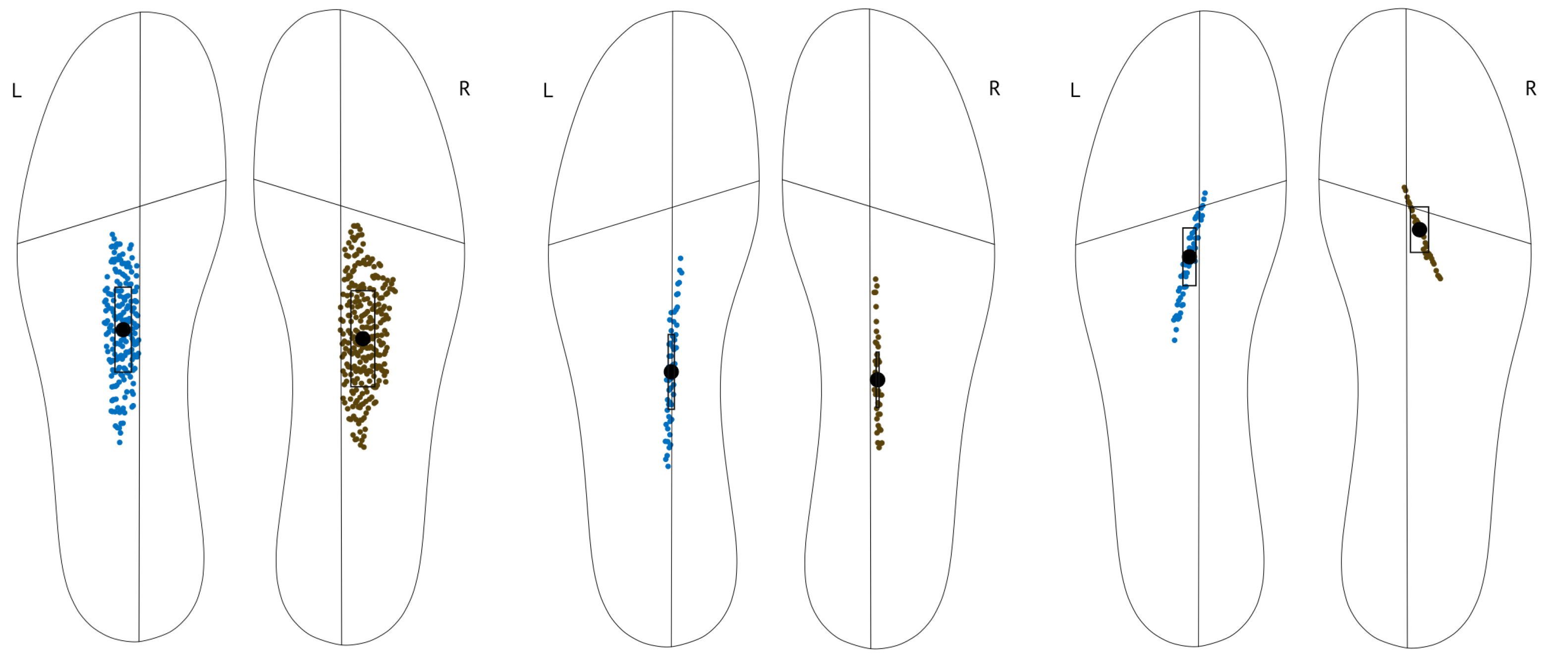
2.4. Experimental Foot Contact Analysis and Modeling—A Pre-Study

The Center of Pressure (CoP) is often used to analyze balance capabilities [5]. In this pre-study we performed CoP measurements using Moticon Pressure Insoles (Moticon GmbH, Munich, Germany) as we expected additional insight into the interaction from these measurements. We recorded standing on one leg in three different situations and for each foot individually. The following results are visualized in Figure 2:
  • Left: Single leg balancing on regular surface
  • Middle: Balancing on the slackline with aligned stance foot
  • Right: Balancing on the slackline with turned stance foot
We see a clear difference between the cases: On flat ground the CoP moves in medial-lateral and in anterior-posterior direction, as is established in the literature. It is different on the slackline: we observe that the CoP does not move within the whole contact plane, but only on a single line. From the aligned and turned foot positioning we can conclude that the direction of this line is determined by the direction of the slackline. Even though the slackline measures 5 cm in width, we see from the measurement data that the CoP does not deviate from the very center of the slackline. We explain this with the fact that the ribbon band of the slackline is able to freely rotate around the center axis between the anchor points. This rotation is barely damped and therefore highly sensitive to shifting the CoP away from the slackline center. Rotating a contact surface, however, greatly reduces the normal force and therefore reduces the non-slipping threshold. We conclude that a small shift of the CoP away from the center of the slackline can already lead to the contact foot slipping off. The very narrow constraints on the CoP together with the continuous vertical and sideways movement of the stance foot explains the difficulty of slackline balancing especially in contrast to walking on a beam.

2.5. Proposed Analysis Method

2.5.1. Slackline Contact Modeling

A foot contact model is required to perform a dynamic motion analysis. A regular planar, non-slipping contact can be described using a total of 8 variables [15]: The contact force F acting in three directions, two variables for the CoP position p in the contact plane and three contact torques M . The forces are constrained by the friction cone to prevent slipping. Taking the measurements presented in Section 2.4 into account, we propose a new contact model for slackline balancing that includes 6 variables. Based on the slackline coordinate system shown in Figure 1 they are:
F = [ F x , F y , F z ] : The contact forces
p = [ p x , 0 ] : The CoP position in along the slackline
M = [ 0 , M y , M z ] : The contact torques in the slackline coordinate system
Zeros are placed where the regular contact model would have had an additional variable. The contact force can still act in all three directions and is still subject to the friction cone. As a consequence of the measurements presented in Figure 2, the CoP position is described by only one free variable instead of two. The Y-coordinate is always zero. The position can no longer be defined in the local coordinate system of the foot, but has to be transformed in the coordinate system of the slackline. Furthermore, we allow only two instead of three contact torques. Again, these are defined by the global position of the slackline and cannot be modeled locally. They act around the vertical axis and are perpendicular to the slackline. As described before, the slackline can freely rotate around the X-Axis and therefore no torque can be applied around this axis.

2.5.2. Subject Modeling and Dynamics Computations

The subject model consists of 17 segments. The length of each segment and the joint locations were estimated from the marker positions of the static trial recording following the Gait-IOR marker set guidelines. Figure 3 shows the static pose recording of the subject at the left and the specific rigid body model in the middle. Joint center positions are visualized in white. Virtual markers are placed on each segment of the model according to the static pose. These virtual markers are used to track the recorded marker data as shown at the right. For the dynamic properties of the model, such as segment mass, inertia or the relative segment CoM position, we refer to the measurements by de Leva [13] and linearly adjust them to the individual segment length. The degrees of freedom (DoF) and the kinematic structure is described in Table 1.
The dynamics of a rigid body system with n d o f DoF using generalized coordinates q are described by the following equation [16]:
H ( q ) q ¨ + C ( q , q ˙ ) = τ
where the matrix H ( q ) R n d o f × n d o f is the generalized inertia matrix that is constructed from the current configuration of the model and the inertia and CoM positions of each segment, C ( q , q ˙ ) R n d o f is the generalized bias force (e.g., gravity or the Coriolis force) and  τ are the generalized forces applied at the joints. This equation holds when the subject is in the air and no external forces are applied. When the model is in contact with the slackline, a contact force F and a contact torque M are acting at the contact point p as derived in Section 2.5.1. We can compute the generalized forces τ c resulting from an external force using:
τ c = G ( q , p ) T M F
where G ( q , p ) is the 6D Jacobian for a point on a body that when multiplied with q ˙ gives a 6-D vector that has the global angular velocity as the first three entries and the global linear velocity as the last three entries. With external contact forces Equation (4) becomes:
H ( q ) q ¨ + C ( q , q ˙ ) = τ + c o n t a c t s τ c
For known joint angles q , joint velocities q ˙ and joint torques τ we are able to compute the joint acceleration q ¨ . This is known as Forward dynamics and implemented in RBDL under the ForwardDynamics function. The contact Jacobean was computed using the CalcPointJacobian6D function. The exact recursive implementation is described in [16].

2.5.3. Optimal Control Problem Formulation

We formulate the dynamic reconstruction of the recorded motion as an OCP. The general multi-phase OCP formulation is derived for example in [17]. We only describe the formulation that was used for the specific problem of motion reconstruction. Unlike our previous work [8,9] where we tracked joint trajectories that were computed beforehand, we now formulate an OCP that tracks the marker positions directly. In the following cost function we minimize the distance between the positions m i of the virtual markers on the model and the 45 recorded marker trajectories m i * over the time t [ 0 , T ] of the motion:
min x , u 0 T i = 0 45 m i ( q ( t ) ) m i * ( t ) 2 d t
with respect to the state vector x and control vector u . They are the same for all phases. The state vector consists of joint angles and joint velocities: x ( t ) = [ q , q ˙ ] . The control vector represents the torques of the actuated joints and all variables of the slackline contact model: u ( t ) = [ τ ( t ) , λ L , λ R ] These are for each foot: three contact forces, two contact torques and the CoP position. All are given in the coordinate system of the slackline as it is shown in Figure 1.
λ R / L = [ F x , F y , F z , T y , T z , p ]
Controls are approximated to be piecewise linear continuous. To retrieve a feasible motion, the EoM must be satisfied and are therefore handled as constraints in the OCP. We reformulate Equation (4) and (6) as first order differential equations for the state vector:
x ˙ ( t ) = f j ( t , q ( t ) , τ ( t ) )
where j N is the phase index. At this point we implemented two formulations: In the first implementation, we used the joint trajectories from the conventional inverse kinematics fit to determine the three different phases of the motion. Figure 4 shows the height of the feet above the ground plotted over time. The slackline is mounted at a rest height of 31 cm. Therefore, we can define a flight phase whenever both feet are above this height. This is indicated in red for the motion at hand. Hence, phases 1 and 3 are contact phases and subject to Equation (6), Phase 2 is a flight phase and subject to Equation (4).
In the second implementation, we defined the whole motion as one phase subject to the contact dynamics (Equation (6)). Additionally, we formulated the following discontinuous path constraint throughout the motion:
r e q ( u ( 0 ) , . . , u ( T ) ) = { λ R , if   Right   Foot   Height   > 0.31   m λ L , if   Left   Foot   Height   > 0.31   m ! = 0 0 , otherwise
This allows the optimizer to determine the exact timing of contact which is fixed within the other  implementation. Additionally, this formulation allows for different contact timings, such as jumping or landing with one foot after the other. This should enable for better marker positions tracking. On the other hand, such a formulation results in non-differentiabilities in the model which might cause numerical problems.
In both implementations, further boundary constraints g ( · ) are implemented for joint angles, velocities and torques and must be respected throughout the motion. The friction cone is implemented as an inequality constraint that requires the normal force to be larger than the horizontal forces. To determine reasonable upper limits for contact forces and torques, we performed a similar jumping motion on two force plates (Bertec, Columbus, OH, USA) and recorded the acting GRF. Limits were set to 1.5 times the measured maximum values. We solve both implementations of the OCP numerically using MUSCOD-II [17,18]. It was developed at the Interdisciplinary Center for Scientific Computing, IWR, Heidelberg University. The state variables are parameterized by the direct multiple-shooting method as it is derived in [19]. The control variables were discretized by piecewise linear continuous functions. On all multiple-shooting intervals, the dynamics of the system are computed in parallel. The same intervals are apply for states and controls. We ensure a continuous solution by imposing continuity constraints at the shooting interval transitions for all state variables. This way, a large but structured nonlinear programming problem (NLP) is obtained. It is solved by an adapted sequential quadratic programming (SQP) method. Further detail can be found in [17]. We expect the first implementation to show better convergence, since discontinuities in the dynamics are supposed to be formulated as phase changes and constraints should be differentiable throughout one phase. However, in practical tests we observed that formulating phase changes as constraints also works in the present case. We did not use a regularization term, which is often used to account for possible redundancies in the contact forces during the double support phases.

2.5.4. Validation

We validate our method by showing that important mechanical properties of the overall system are satisfied due to the fact that Newton’s EoM have been formulated as constraints to the OCP. This includes:
  • Horizontal momentum is conserved during the flight phase
  • Gravity is the only acceleration acting on the CoM during the flight phase
  • Angular momentum is conserved during the flight phase
  • The change of momentum is proportional to the sum of external forces
  • The change of angular momentum is equal to the sum of all acting torques.
With the change of momentum being equal to the CoM acceleration c ¨ times the subject mass m and  L being the angular momentum, we reformulate Newton’s EoM:
c ¨ m = λ L / R F
L ˙ = λ L / R ( M + ( p i c ) × F )
where p is the point where the force is acting. During all phases Equations (11) and (12) must hold. For the contact phases we can compute the left hand side of Equations (11) and (12) using the CalcCenterOfMass function of RBDL and the right hand side from result values of  λ L / R of the OCP result.

3. Results and Discussion

Both implementations converged. Due to the problem’s complexity, we were numerically limited to ≈80 shooting nodes. We chose 40 multiple-shooting intervals per 1 s of motion and reconstructed around 2 s of motion. Other choices are possible, but we found that the computation time drastically increases with more shooting nodes and that the solver is not always able to find solutions for less shooting nodes per second of motion. As expected, the single-phase implementation resulted in a slightly lower tracking error. Therefore we present the results for the single-phase implementation. The resulting motion and the interaction forces (visualized as yellow arrows) are shown in Figure 5. Contact and flight phases are clearly distinguished. We see that the subject equally used both feet to initiate and land the jump and that contact torques were acting to build the necessary angular momentum for the rotation. The feet were aligned with the Slackline during the first contact phase and were turned perpendicular for landing.
We present the fitting error of our model to the measured marker data: Figure 6 shows the average marker residuum on the top and the frame by frame error on the bottom. Overall we achieved an average tracking error of 3 cm per marker. This accuracy is similar to the least squares kinematic fit of the conventional analysis that was used to initialize the OCP and to what is reported in the literature. The largest deviations occur for the two shoulder markers (L_SAE and R_SAE). One reason for this is that the arms were aligned to the upper body during the static pose on which the model is based. During slacklining, however, the arms are turned 90 ° compared to this pose and mainly parallel to the ground which results in skin and marker movement relative to the bone and shoulder joint. This offset is visible throughout the motion. Additionally, the shoulder is modeled as a spherical joint with only three DoF. In reality this joint is much more complex and also has translational DoF. This currently limits the tracking accuracy; however, a more precise kinematic shoulder model could be used.
Figure 7 shows the CoM velocity and acceleration throughout the motion. The conventional motion analysis is plotted in green, the OCP result of the proposed method in purple. The most apparent differences occur during the flight phase when no forces are acting. As derived in Section 2.5.4, we expect constant accelerations and conservation of momentum in horizontal direction. Gravity should be the only force acting in vertical direction. This is indeed the case for the OCP result but is not given for the conventional analysis. Looking at the CoM acceleration we see values of up to 0.5 m s 2 in X direction and 0.7 m s 2 in Y direction during the flight phase. With the maximum values during the whole motion being 2.5 m s 2 and 3.5 m s 2 , respectively, this leads to an estimated relative error of up to about 20% for the conventional analysis.
Angular momentum is plotted in Figure 8. It should also be conserved during the flight phase and the change should be equal to zero when no external torques are acting. Again, we observe the desired properties for the optimized motion. The conventional analysis shows high variability during the flight phase and errors in the range of 30% in the horizontal plane.
On the left of Figure 9 we plotted the contact forces for each foot stacked on top of each other and the CoM acceleration times the subject mass as a dashed line. We can see that they exactly match and that Equation (11) holds. On the right we have the same result for the contact torques. Again, Equation (12) is satisfied throughout the motion. This shows that the optimization result follows Newton’s EoM also during the contact phases. The resulting forces are consistent with the CoM acceleration and the resulting contact torques and CoP position are consistent with the change of angular momentum. We have established that the dynamics of our optimization framework are physically feasible and can further analyze the motion itself.
We do so by looking at the sideways and vertical direction and forces and torques individually. As shown in Figure 1 the X-Axis is aligned with the slackline, the Y-Axis perpendicular and the Z-Axis in vertical direction. The Y direction is particularly interesting since the subject is very unstable due to the slackline and torques can only be applied controlling the contact force. Looking at the CoM acceleration we see spring-like behavior before and after the jump. The subject is constantly swinging sideways. Amplitudes are small when the subject is in balance, larger after the landing and decreasing during the stabilization process. The oscillation frequency appears to be the same throughout the motion. The interaction forces of both feet point into the same direction, back towards the center of the anchor points of the slackline. We also observe spring spring-like properties before and after the jump in the vertical direction. The slackline model proposed by Paoletti and Mahadevan [1] models the force of the slackline also as a spring with the direction towards the resting position. However, they only considered sideways movement and did not take vertical movement of the subject into account. The lower left plot of Figure 9 shows the sum of contact torques and the sum of the torque generated from the contact forces. We see that the subject initiates the rotation applying contact torques when the feet are parallel during the first contact phase. After landing, the feet are perpendicular to the slackline and the contact forces are used to decrease the rotation.
In the future, we plan to apply the method to several other slackline tricks such as front or backflips, chest or pelvis bounces. For this task we plan to introduce other contact points for example at the hands, the chest or the pelvis. Another possibility would be a thorough gait analysis of slackline walking and the comparison to flat ground walking regarding stability parameters. We intend to reconstruct a full gait cycle and gain more insight in human balancing strategies. Furthermore, we want to analyze the resulting contact forces relative to the foot positions and develop a thorough spring model of the slackline. We showed that the current model by Paoletti and Mahadevan [1] is oversimplified as it does not take the whole range of motion of the slackline into account.

4. Conclusions

In this work we derived a general contact model for slackline balancing and demonstrated how it can be applied to analyze jumping on slackline. We employed the model inside an optimization framework to reconstruct the dynamics of a slackline jump with 180 ° rotation. We successfully implemented a multi-phase and a single-phase formulation leading to almost equivalent results. We found that the resulting motion has similar fitting error to the markers when compared to the inverse kinematics approach, but is physically feasible and time consistent. The advantage of our approach becomes apparent during the flight phase of the motion and when comparing the CoM and angular momentum dynamics. We found variations of up to 30% for the conventional method. Due to numeric complexity and the high amount of variables necessary to formulate the OCP, this method is limited to a few seconds of motion. This might limit the application to compare longer slackline motions of beginners and experts as initially intended. However, we can apply it to interesting parts of motion and analyze specific movements connected to balance recovery.

Author Contributions

Conceptualization, K.S. and K.M.; Formal analysis, K.S.; Funding acquisition, K.M.; Investigation, K.S.; Project administration, K.M.; Supervision, K.M.; Writing—original draft, K.S.; Writing—review & editing, K.M. All authors have read and agreed to the published version of the manuscript.

Funding

Funding by the Carl Zeiss Foundation within the “Heidelberg Center for Motion Research” is gratefully acknowledged.

Acknowledgments

We want to thank the Simulation and Optimization research group of the IWR at Heidelberg University for giving us the possibility to work with MUSCOD-II. We also want to acknowledge financial support by the Baden-Württemberg Ministry of Science, Research and the Arts and by Ruprecht-Karls-Universität Heidelberg.

Conflicts of Interest

The authors declare no conflict of interest.

Abbreviations

The following abbreviations are used in this manuscript:
CoMCenter of Mass
CoPCenter of Pressure
DoFDegrees of Freedom
EoMEquation of Motion
GRFGround Reaction Forces
L_SAELeft Scapula Acromial Edge
n d o f Number of Degrees of Freedom
NLPNonlinear Programming Problem
RBDLThe Rigid Body Dynamics Library
R_SAERight Scapula Acromial Edge
OCPOptimal Control Problem
SQPSequential Quadratic Programming
ZMPZero Moment Point

References

  1. Paoletti, P.; Mahadevan, L. Balancing on tightropes and slacklines. J. R. Soc. Interface R. Soc. 2012, 9, 2097–2108. [Google Scholar] [CrossRef] [PubMed] [Green Version]
  2. Stein, K.; Mombaur, K. Performance indicators for stability of slackline balancing. In Proceedings of the IEEE/RAS International Conference on Humanoid Robots (Humanoids 2019), Toronto, ON, Canada, 15–17 October 2019. [Google Scholar]
  3. Winter, D. Human balance and posture control during standing and walking. Gait Posture 1995, 3, 193–214. [Google Scholar] [CrossRef]
  4. Sutherland, D. The evolution of clinical gait analysis: Part II Kinematics. Gait Posture 2002, 16, 159–179. [Google Scholar] [CrossRef]
  5. Thompson, L.; Badache, M.; Cale, S.; Behera, L.; Zhang, N. Balance performance as observed by center-of-pressure parameter characteristics in male soccer athletes and non-athletes. Sports 2017, 5, 86. [Google Scholar] [CrossRef] [PubMed] [Green Version]
  6. Xu, F.; Li, X.; Shi, Y.; Li, L.; Wang, W.; He, L.; Liu, R. Recent Developments for Flexible Pressure Sensors: A Review. Micromachines 2018, 9, 580. [Google Scholar] [CrossRef] [PubMed] [Green Version]
  7. Karatsidis, A.; Bellusci, G.; Schepers, H.M.; de Zee, M.; Andersen, M.S.; Veltink, P.H. Estimation of ground reaction forces and moments during gait using only inertial motion capture. Sensors 2016, 17, 75. [Google Scholar] [CrossRef] [PubMed] [Green Version]
  8. Emonds, A.L.; Funken, J.; Potthast, W.; Mombaur, K. Comparison of Sprinting with and without Running-Specific Prostheses Using Optimal Control Techniques. Robotica 2019, 37, 2176–2194. [Google Scholar] [CrossRef]
  9. Stein, K.; Mombaur, K. Optimization-Based Analysis of a Cartwheel. In Proceedings of the 7th IEEE International Conference on Biomedical Robotics and Biomechatronics (Biorob), Enschede, The Netherlands, 26–29 August 2018; pp. 909–915. [Google Scholar]
  10. Leardini, A.; Biagi, F.; Merlo, A.; Belvedere, C.; Benedetti, M.G. Multi-segment trunk kinematics during locomotion and elementary exercises. Clin. Biomech. 2011, 26, 562–571. [Google Scholar] [CrossRef] [PubMed]
  11. Felis, M. Modeling Emotional Aspects in Human Locomotion. PhD Thesis, Heidelberg University, Heidelberg, Germany, 2015. [Google Scholar]
  12. Sugihara, T. Solvability-Unconcerned Inverse Kinematics by the Levenberg- Marquardt Method. IEEE Trans. Robot. 2011, 27, 984–991. [Google Scholar] [CrossRef]
  13. De Leva, P. Adjustments to Zatsiorsky-Seluyanov’s segment inertia parameters. J. Biomech. 1996, 29, 1223–1230. [Google Scholar] [CrossRef]
  14. Jensen, R.K. Body segment mass, radius and radius of gyration proportions of children. J. Biomech. 1986, 19, 359–368. [Google Scholar] [CrossRef]
  15. Elftman, H. Forces and Energy Changes in the Leg During Walking. Am. J. Physiol. 1939, 125, 339–356. [Google Scholar] [CrossRef] [Green Version]
  16. Felis, M.L. RBDL: An efficient rigid-body dynamics library using recursive algorithms. Autonomous Robots 2016, 1–17. [Google Scholar] [CrossRef]
  17. Kuhl, P.; Ferreau, J.; Albersmeyer, J.; Kirches, C.; Wirsching, L.; Sager, S.; Potschka, A.; Schulz, G.; Diehl, M.; Leineweber, D.; et al. MUSCOD-II Users’ Manual; Interdisciplinary Center for Scientific Computing (IWR): Heidelberg, Germany, 2001. [Google Scholar]
  18. Leinweber, D.; Bauer, I.; Bock, H.; Schloeder, J. An efficient multiple shooting based reduced SQP strategy for large-scale dynamic process optimization. Part I: Theoretical aspects. Comput. Chem. Eng. 2003, 27, 157–166. [Google Scholar] [CrossRef]
  19. Bock, H.; Plitt, K. A Multiple Shooting Algorithm for Direct Solution of Ooptimal Control Problems; Pergamon Press: Oxford, UK, 1984; pp. 243–247. [Google Scholar]
Figure 1. Left: A subject balancing on a slackline. An elastic ribbon band is mounted between two anchor points. The foot contact is able to move sideways and in up and down direction. Right: Kinematic motion capture data of slackline balancing. The coordinate system definition is used throughout this work.
Applsci 10 01094 g001
Figure 2. Center of Pressure recording of different single leg balancing tasks. We recorded both legs individually using Moticon Pressure Insoles. Left: Single leg balancing on regular surface. The CoP is moving in the anterior-posterior and in medial-lateral direction. Middle: Balancing on the slackline with aligned stance foot. Right: Balancing on the slackline with turned stance foot. The CoP is constrained by the direction of the slackline and to a single line.
Applsci 10 01094 g002
Figure 3. Left: The static pose of the subject. Middle: The rigid body model in Puppeteer. Joint centers are visualized in white. Virtual markers were placed on the model following the static pose. Right: Inverse kinematic fit of the model to a slackline pose.
Applsci 10 01094 g003
Figure 4. Feet positions are plotted against time. The rest height of the slackline is 31 cm. We determine the times of contact and flight phases when both feet are higher than the slackline. The flight phase is indicated in red.
Applsci 10 01094 g004
Figure 5. The result of this work: A fully dynamic reconstruction of a jumping motion with rotation. The contact forces and torques are visualized.
Applsci 10 01094 g005
Figure 6. Top: Average marker error for all 45 markers. Largest deviations occur for the shoulder markers. This is due to the fact that the model is based on a N-Pose capture and the slackline motion mainly had a T-Pose like arm positioning. Bottom: Frame by frame marker error.
Applsci 10 01094 g006
Figure 7. Center of Mass velocity and acceleration in global coordinates during the motion. Results from the conventional method are plotted in green, the proposed method is plotted in purple. During the flight phase all horizontal accelerations are supposed to be zero and the according velocities should be constant. We see inconsistencies and changes in the range of 20% for the conventional method whereas the proposed method is physically feasible.
Applsci 10 01094 g007
Figure 8. Angular Momentum and Change of Angular Momentum around the Center of Mass. Similar to Figure 7 we see constant values during the flight phase and zero values of the derivative for the proposed method. Values computed with the conventional method are not respecting Newtons EoM.
Applsci 10 01094 g008
Figure 9. Left: Sum of contact forces and Center of Mass acceleration times subject mass. Right: Sum of contact torques and torques produced by the contact forces plotted against the change of angular momentum. Equations (11) and (12) are satisfied throughout the motion.
Applsci 10 01094 g009
Table 1. Description  of the kinematic structure of the model with all degrees of freedom.
SegmentParentDoF
PelvisRoot6d Floating Base
Lower TrunkPelvisRY, RZ
Upper TrunkLower TrunkRX, RY
HeadUpper TrunkRZ
Upper ArmUpper TrunkRX, RY, RZ
Lower ArmUpper ArmRY, RZ
HandLower ArmFixed
ThighPelvisRX, RY, RZ
ShankThighRY
FootShankRY

