Article

Data-Efficient Domain Adaptation for Semantic Segmentation of Aerial Imagery Using Generative Adversarial Networks

1
Robotics and Internet of Things Laboratory, College of Computer and Information Sciences, Prince Sultan University, Riyadh 11586, Saudi Arabia
2
Research Laboratory Smart Electricity & ICT, SEICT, LR18ES44, National Engineering School of Carthage, University of Carthage, Tunis 2035, Tunisia
3
CISTER, INESC-TEC, ISEP, Polytechnic Institute of Porto, 4200-465 Porto, Portugal
*
Author to whom correspondence should be addressed.
Appl. Sci. 2020, 10(3), 1092; https://doi.org/10.3390/app10031092
Submission received: 17 December 2019 / Revised: 28 January 2020 / Accepted: 29 January 2020 / Published: 6 February 2020
(This article belongs to the Special Issue Applications of Computer Vision in Automation and Robotics)

Abstract

:
Despite the significant advances noted in semantic segmentation of aerial imagery, a considerable limitation is blocking its adoption in real cases. If we test a segmentation model on a new area that is not included in its initial training set, accuracy will decrease remarkably. This is caused by the domain shift between the new targeted domain and the source domain used to train the model. In this paper, we addressed this challenge and proposed a new algorithm that uses Generative Adversarial Networks (GAN) architecture to minimize the domain shift and increase the ability of the model to work on new targeted domains. The proposed GAN architecture contains two GAN networks. The first GAN network converts the chosen image from the target domain into a semantic label. The second GAN network converts this generated semantic label into an image that belongs to the source domain but conserves the semantic map of the target image. This resulting image will be used by the semantic segmentation model to generate a better semantic label of the first chosen image. Our algorithm is tested on the ISPRS semantic segmentation dataset and improved the global accuracy by a margin up to 24% when passing from Potsdam domain to Vaihingen domain. This margin can be increased by addition of other labeled data from the target domain. To minimize the cost of supervision in the translation process, we proposed a methodology to use these labeled data efficiently.

1. Introduction

The semantic segmentation task provides for every pixel in the input image a label that defines its semantic class. In remote sensing context, the semantic segmentation of aerial images has an increasing potential for many tasks and applications, like analysis and management of road traffic, monitoring of urban and rural areas, fast interactions in case of emergency, and so on. The growing adoption of Unmanned Aerial Vehicles (UAVs) is behind this increasing potential. High-resolution images can be collected using UAVs from different points of view and processed by the semantic segmentation algorithms to promote the automatic analysis of surveyed scenes.
Since the emergence of Convolutional Neural Networks (CNNs), the area of image analysis algorithms has shown a considerable improvement in accuracy [1,2,3,4,5,6,7]. This affected directly the area of semantic segmentation and paved the way towards a variety of CNN-based architectures, like SegNet [8], fully connected network (FCN), PSPNet [9], U-Net [10] and DeepLab [11]. Empirically, if we build a robust dataset and we train on it one of the state-of-the-art algorithms, we will get an accuracy that easily surpasses 80%.
Despite this exciting efficiency, a notable challenge is blocking the use of semantic segmentation algorithms in real cases. In fact, the accuracy of the model will be high only on images belonging to the same domain of the dataset used in training (object representation, resolution, sensor type, lighting conditions). If we test this model in another domain (images collected under conditions different from those of the training set), the accuracy decreases remarkably. This decrease is caused by the domain shift existing between the target and the source domain. Figure 1 shows a real case scenario in which we want to test the semantic segmentation model on a domain different from the source. A considerable shift is remarked between the two domains (location is changed, image coding is changed, resolution is changed).
The straightforward solution to mitigate this intriguing limitation is to train our model on a labeled dataset constructed from the target domain in a supervised or a semi-supervised way [12]. However, this method is costly and time-consuming. To illustrate this, we can note that pixel-labeling of an image from Cityscapes dataset takes nearly 90 minutes on average [13]. The size of the image is 2040 by 1016 pixels. To reduce the labeling time, we can benefit from human crowd intelligence by distributing the labeling task over a set of human crowds [14]. Every set will be allocated to the labeling of one class. This reduces the cost of generating the semantic labeled dataset on the target. Nevertheless, since such solutions are not always immediately available, it is still useful to search for a data-efficient solution of domain adaptation that uses only a minimal set of images for supervision of the domain transfer.
Domain adaptation is a separate area in machine learning whose objective is to learn how a model performance on a source data distribution can be improved on another target data distribution. Domain adaptation helps in mitigating the domain shift between the target domain data and the source domain data used in training. Typically, a mapping function is designed between the target domain and the source domain. Deep learning models have been used by the recent methods of domain adaptation for the training of such a mapping function [15,16,17,18].
Motivated by the current breakthrough made by GANs (Generative Adversarial Networks) [19,20], we developed a data-efficient domain adaptation algorithm based upon an architecture of two GAN networks. Our method aims at handling the case indicated in Figure 1 as well as other cases of the same nature. Our technique is based on converting the image that we want to segment from the target domain to the source domain by passing it through two consecutive GAN networks. The two generative adversarial networks are trained separately. The first GAN network converts the chosen image from the target domain to a semantic segmentation label. The second GAN network converts this semantic label into the source domain. The generated image is proven to conserve the semantic map of the first image and to mimic the source domain characteristics. It will be used as an input to the segmentation model already trained on the source dataset and will generate a better segmentation label, as proven by the experiments we made. The accuracy of final segmentation using our algorithm can be increased by addition of labeled data from the target domain. A methodology is described to use the labeled data efficiently to minimize the cost of supervision in our algorithm. Our work has the following contributions: (1) Our approach is confirmed to mitigate the problem of domain shift for semantic segmentation by a significant margin that can increase with an efficient addition of labeled data from the target domain. (2) The method is validated using ISPRS semantic labeling dataset through the establishment of cross-domain semantic segmentation between Vaihingen and Potsdam datasets. (3) GANs are introduced as a favorable solution for analyzing aerial imagery.
The following is the organization of our paper: Section 2 provides a summary of the related works in the domain adaptation area within semantic segmentation. Section 3 will make an introduction to GANs. Section 4 will describe the different parts of our proposed method. Section 5 will present the experiments made to validate our method and discuss its effectiveness within domain adaptation of semantic segmentation in aerial imagery. Finally, our work is concluded in Section 6, which also deduces the possible extensions of our method.

2. Related Works

In this section, we will discuss the works that treated domain adaptation within semantic segmentation. Generally, it is assumed, in the machine learning context, that the test and the training datasets are belonging to the same distribution. However, there is substantial discordance between them in real cases. This discordance reduces the model’s efficiency out of its training domain. Domain adaptation techniques are used mitigate this discordance and to make the model generalizes better over multiple domains.
In computer vision, efforts made on domain adaptation have been more focused on regression and classification tasks [21] not on semantic segmentation. For example, many works treated the training of the models on online images for the classification of objects in reality [22]. Recent works in this area are focusing on improving the adaptability of deep learning algorithms [15,16,23,24,25].
In semantic segmentation, most of the domain adaptation works are geared towards the use of simulated data [26,27,28,29,30,31]. In fact, domain adaptation was expected to be used by these works for the improvement of the efficiency of segmentation on real images through the training of the semantic segmentation model on pure synthetic data. FCNs in the wild [32] is one of the earliest works. It uses a pixel-level adversarial loss to guide the model to learn the domain-invariant properties. This aims at making the adversarial classifier not to differentiate between the target and the source domains. The goal is to make its performance equal on the two domains. Hoffman et al. [26] designed CyCADA, which is a model that changes synthetic data (source domain images) into real data style (target domain images) using CycleGAN. The segmentation model is then fed with the converted images to improve its accuracy on dealing with real photos. On the other hand, Zhang et al. [33] pointed out that a curriculum-style learning technique helps in reducing the domain shift. They deduced the target data properties by joining the learning of global label distribution with the learning of local distributions over landmark superpixels. The segmentation network was then trained through regularizing it to follow these features. Sankaranarayanan et al. [34] treated the problem differently by taking the source and the target images as input to an auto-encoder network that processes and regenerates them before feeding them to the segmentation model. CGAN architecture is another approach introduced by Tsai et al. [35] that makes addition of random noise into the source data giving it as input to the segmentation model. They proved that this technique enhances the model’s efficiency on the target domains. Huang et al. [36] proposed to train independently two networks for the target and the source domains. The training of the target model is done through its regression into the source model weights since the target domain is without labels. It should be noted that the calculation of an adversarial loss in each layer of both networks is done.
Aerial imagery has its peculiarities that should be considered. Therefore, a dedicated work that takes into consideration its peculiarities should be investigated. Recently, three works targeted the domain adaptation in semantic segmentation of aerial imagery. All of them used an unsupervised approach. The first work is the algorithm proposed by Benjdira et al. [4]. They introduced a GAN architecture to map images in an unsupervised way from the source domain to the target domain without the need for paired data. After that, they translated the source domain dataset into the target domain. Then, the translated dataset is used to fine-tune the segmentation model to enhance its ability to treat images from the target domain. The second work is the work proposed by Tasar et al. [37]. They adopted the same algorithm of Benjdira et al. [4] but changed the GAN architecture into another architecture named ColorMapGAN. This architecture converts the source images into images that the spectral distribution is similar to the target spectral distribution but conserves the semantic information of the source. The third work is introduced by Fang et al. [38]. They made a category-sensitive domain adaptation (CsDA) using a geometry-consistent GAN (GcGAN) embedded into a co-training adversarial learning network (CtALN). Their method is currently the state of the art in unsupervised domain adaptation in semantic segmentation of aerial imagery. Up to our knowledge, no one has treated the domain adaptation in semantic segmentation of aerial imagery using a supervised approach. We aim in this work to target this limitation and to study the implementation of a supervised domain adaptation algorithm based on the concatenation of two GAN networks. We only use a reduced amount of labeled data to guide the model during the training. To demonstrate our algorithm’s efficiency, we tested it on the ISPRS semantic segmentation dataset [39]. We performed the domain adaptation for a semantic segmentation network from Potsdam (as source) to Vaihingen (as target).

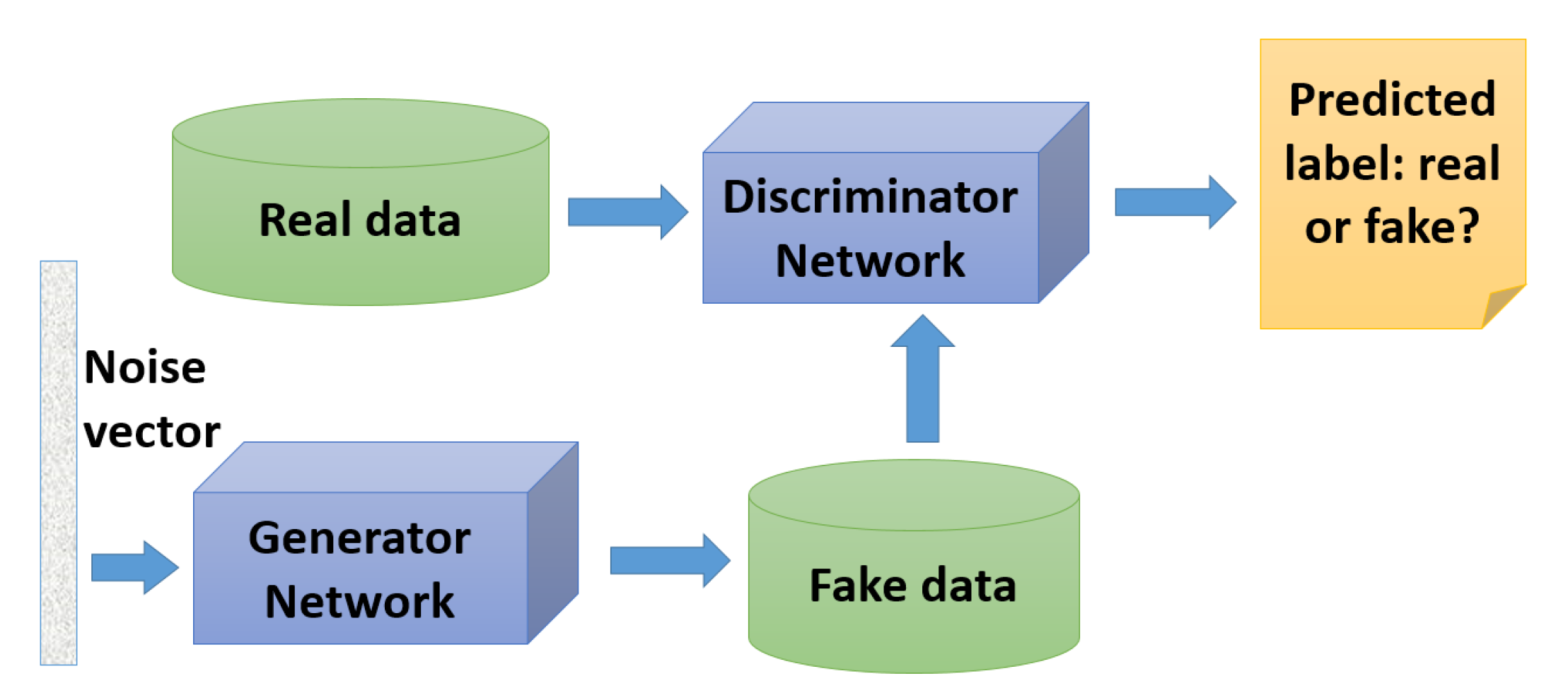
3. Generative Adversarial Networks (GANs)

3.1. The Generator and the Discriminator

The popularity of GANs has continued to increase because they have many addressable applications. Goodfellow et al. [19] introduced GAN in 2014. A GAN is composed of two separate networks: the generator and the discriminator. During the training process, the generator learns how to generate data that mimics real data, whereas the discriminator learns how to differentiate real data from fake data produced by the generator. The training is operated jointly so that both are competing and playing an adversarial zero-sum game.
During the training, the generator is trying continuously to generate fake data that deceives the discriminator so that it classifies them as real. However, the discriminator is trying continuously to detect the fake data and not to classify them as real. To solve the adversarial zero-sum game during the training, game theory theorems are used. Figure 2 indicates the standard architecture of the GAN network.
During training, both networks engage in competition until a Nash equilibrium is reached. In game theory, Nash equilibrium is a status where no player is able improve or deviate his payoff [40].
Equation (1) shows the objective function of GAN:
m i n G m a x D V ( D i s , G e n ) = I E X P r e a l _ d a t a ( X ) [ l o g D i s ( X ) ] + I E z P z ( z ) [ l o g ( 1 D i s ( G e n ( z ) ) ) ]
where G e n denotes the generator cost function which is trained through the maximization of D i s ( G e n ( z ) ) . On the other hand, D i s represents the discriminator cost function which is trained through the minimization of D i s ( G e n ( z ) ) . While X is the image that is obtained from the distribution of real data p r e a l _ d a t a . The noise vector obtained from distribution p z is denoted by z whereas G e n ( z ) indicates the fake image that is produced by the generator. Additionally, I E X P d a t a ( X ) represents the expectation on X, which is acquired by the distribution P r e a l _ d a t a ( X ) . Both Dis and Gen play the two-player minimax game using the value function V ( G e n , D i s ) [19].
Generative adversarial networks have many applications and implementations [41] with image-to-image translation being the application that may be the most attractive to be used in the domain adaptation’s context. The use of GANs in the area of image-to-image translation is further discussed in the following subsection.

3.2. translation from Image-to-Image using GANs

The translation of an image from one domain to another has been the target for many GAN architectures [20,42,43,44]. Translation of images can be paired [20] or unpaired [45].

3.2.1. Paired Image-to-Image Translation

In this particular area, the GAN model must be trained using labeled pairs of images. With X being the source data, Y being the target data and N being the number of samples in each dataset, each pair of corresponding images { x i } i = 0 N and { y i } i = 0 N will be used by the model to learn in a supervised way how to translate between X and Y domains. Currently, Pix2pix [20] is the most known model for paired image-to-image translation.

3.2.2. Unpaired Image Translation
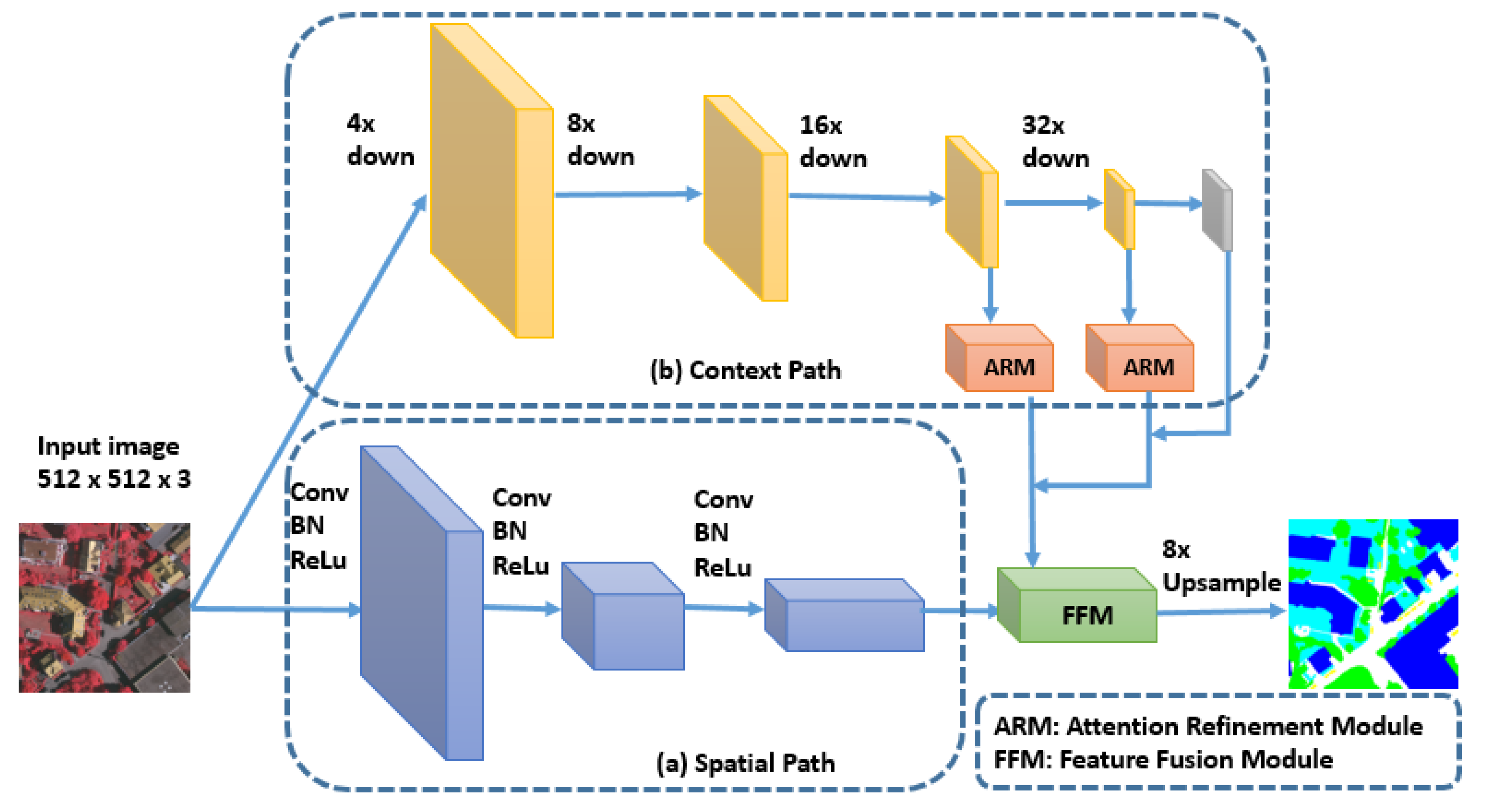
GAN is used in unpaired image translation to convert between two sets of images through an unsupervised training. With X being the source data, Y being the target data, N being the number of samples in the source dataset and M the number of samples in the target dataset, { x i } i = 0 N and { y i } i = 0 M do not correspond with each other and can randomly be obtained from the related domain set. Currently, CycleGAN [45] is the most known model for unpaired image-to-image translation.

4. Proposed Method

4.1. The GAN Architecture

Our method aims at translating images from the target domain to the source domain using two GAN networks as illustrated in Figure 3. The entire procedure makes the target domain images imitate the source domain characteristics, which include the quality of images, types of sensors and resolution, among others. The mapping process between the target and the source is done in two steps. First, the chosen image from the target is mapped into semantic label using the first GAN Network. Then, the generated label is mapped using the second GAN network into another image that looks like images from the source domain distribution. The two networks are trained separately using paired datasets. We used a modified architecture from the standard GAN that is inspired by some recent architectures [20,45].
The first GAN Network is designed by substituting the noise vector in the traditional GAN Network by images from the target distribution. The data generated by this GAN Network are the semantic label of the entry image. The training process is done using a small-sized dataset constructed from a few samples from the target domain and their semantic labels. The mapping function of the generator, G : X L , learns through an adversarial training how to produce the semantic label L of the target image X. Because the target is supposed to have a minimal set of labels, we assume that the provided labeled images are only a few significant samples from the target dataset. We mean by significant samples the existence of two constraints during the selection of the images. First, the sampled images should contain all the semantic classes of the dataset. Second, for each class, we should choose samples with the most available representations of the class inside the dataset. The discriminator D learns during the adversarial training how to differentiate between real pairs ( X , L o r i g i n a l ) and the fake pairs ( X , L g e n e r a t e d ) . While the discriminator improves its ability to detect fake pairs from real pairs, the generator improves its ability to generate the true semantic labels of the input image. The architecture of the generator and the discriminator in the first GAN network is illustrated in Figure 4.
Concerning the generator, it is an encoder-decoder architecture with skip-connections. It is similar to U-Net [10] architecture. Eight convolutional layers are used for downsampling in the encoder part and similarly, eight deconvolutional layers are used for upsampling in the decoder part. Leaky ReLu [46] is used as the activation layer for all the layers of the encoder except the first one. Leaky ReLu is identical to the standard ReLu in the positive region. However, in the negative part, it has a small slope α . Explicitly, it is defined as L e a k y R e L u ( x ) = x , if x > = 0 ; and as L e a k y R e L u ( x ) = α x , if x < 0 . α has a small value, which gives small gradient where x < 0 . The encoder part ends by giving us a small feature vector of size ( 1 × 1 × 512 ) . This feature vector will pass through the decoder part to rebuild the original feature vector. We used skip connections to concatenate every layer output in the encoder part with the corresponding layer in the decoder part. ReLu is used as the activation function for all the layers of the decoder. Batch normalization [47] is used after every layer of network except the first layer of the encoder and the last layer of the decoder. We used dropout [48] in the first three layer of the decoder to reduce overfitting. We apply t a n h as an activation function to the last layer of the decoder to get the predicted label for the input image.
Concerning the discriminator, it takes as input pairs of images from two sets. The first set is images from the target dataset associated with their real label ( X t a r g e t , L o r i g i n a l ) . Data from this set should be classified by the discriminator as real pairs of data. The second set is images from the target dataset associated with the generated label from the generator network ( X t a r g e t , L g e n e r a t e d ) . Data from this set should be classified by the discriminator as fake pairs of data. In the discriminator, five convolutional layers are used to encode the pair of images ( X , L ) into a feature vector of size ( 30 × 30 × 1 ) . Then we apply the Sigmoid activation function to this feature vector to get the final binary output of the discriminator {0: fake pairs, 1:real pairs}. As with the encoder part of the generator, we used Leaky ReLu [46] and Batch normalization [47] in every layer except the final one.
Concerning the second GAN Network, it is similar to the first GAN Network. It has a generator and a discriminator as detailed in Figure 3. The architecture of the generator is identical to the architecture of the first generator (See Figure 4) except that it has as input a semantic label and generates an image that imitates images taken from the source dataset. The architecture of the discriminator is also identical to the discriminator of the first GAN (See Figure 4) except that it takes as input pairs of images from two sets. The first set consists of semantic labels associated with their corresponding images from the source dataset ( L s o u r c e ) , X o r i g i n a l ) . The second set consists of semantic labels associated with the generated images from the generator network ( L s o u r c e ) , X g e n e r a t e d ) .

4.2. The Description of the Algorithm

The algorithm adopted to mitigate the domain shift between the source and the target is based on the GAN architecture provided in Figure 3. It is divided into five steps that are illustrated in Figure 5.
There are five steps in the algorithm. Step one begins by the training of a segmentation model on the source domain dataset. The accuracy of the segmentation model could easily get to over 80% if there is a well-structured dataset. In Step 2, we pick out some significant samples from the target domain and label them. The samples are significant if they meet two requirements. First, all the classes should exist in the samples. Second, the most common class representations should be presented. In Step 3, we use these samples to train the first GAN network. Step four makes the training of the second GAN network based on the source dataset provided with labels. Step five is the step where we use our proposed GAN to segment images from the target domain. This step is divided into five sub-steps. In the first sub-step, we pick out any image from the target domain that we want to segment. Then, we pass it into the generator of the first GAN network to translate it into labels. After that, we pass the generated label into the generator of the second GAN network. This will convert it into an image that imitates images from the source domain. In the fourth sub-step, we pass this generated image into the segmentation network trained in Step 1. We will get then the semantic segmentation map of the image.

4.3. Problem Formulation

This section presents the formal modelling of our algorithm. We consider the domain adaptation problem from the target data X T to the source data X S . The source data are provided with full semantic labels Y S while the target data are not initially provided with labels. The first step of the algorithm is concerned with training a semantic segmentation model M S on the source data. The following equation is correspondent to the source model M S with the use of the cross-entropy loss:
L M S ( M S , X S , Y S ) = I E ( x s , y s ) ( X S , Y S ) c = 1 C I l [ c = y s ] l o g ( S o f t m a x ( M S ( c ) ( x s ) ) )
where I E ( x , y s ) ( X S , Y S ) denotes the expectation on x s , y s , which is drawn by the X S and Y S distribution. C is the number of classes of the segmentation task. I l [ c = y s ] represents the loss for the class c separated from other classes. Due to the advancements in the semantic segmentation field, M S could have a good accuracy if the source data are well constructed. However, when we use this model to segment images from the target domain, the accuracy will decrease because of the domain shift that exists between the source and the target. Hence, we will apply our proposed algorithm and begin by picking out significant samples from the target domain and labeling them. This small dataset will guide the mapping process from the target to the source. It will be used to train the first GAN Network, which will learn through an adversarial loss how to generate pixel-wise labels of the target images.
The mapping model from the target domain to the semantic labels G T L is trained for a segmentation task in an adversarial manner. The discriminator D T L will be trained on the other side to detect fake pairs of data from the real ones. This GAN model can be seen as a standard GAN where we applied three modifications. First, we substituted the noise vector by input images from the target domain. Second modification is to set the output of the GAN to semantic segmentation labels of the input image. Third, is to set the input for the discriminator as pair of image for the target domain x t , and semantic label real or generated by the discriminator ( l t _ r e a l or l t _ g e n e r a t e d ).
Also, the GAN model can be treated as a modification of a conditional GAN [49]. Generally, conditional GANs or cGANs make a mapping between an input and an output. The input are formed by an image x from a distribution X concatenated to a noise vector z. The output is an image y from a distribution Y. The mapping is formulated by G c G A N : { x , z } y and the loss function of a conditional GAN can be formulated as:
L c G A N ( G , D , X , Y , z ) = I E ( x X , y Y ) [ l o g D ( x , y ) ] + I E ( x X , z ) [ l o g ( 1 D ( x , G ( x , z ) ) ]
During the training, G (the generator) is trying to minimize this loss, whereas D (the discriminator) is trying to maximize it. The loss function can be expressed more clearly as:
L = a r g m i n G m a x D L c G A N ( G , D , X , Y , z )
As proven in [20], mixing this GAN objective with L 1 loss gives beneficial results. In fact, this helps the generator to be more able to fool the discriminator by being closer to the ground truth in an L 1 sense. This loss does not affect the discriminator. The L 1 loss related to the cGAN can be expressed as:
L L 1 = I E ( x X , y Y , z ) [ y G ( x , z ) 1 ]
The final objective of the cGAN can be expressed as:
L = λ 1 a r g m i n G m a x D L c G A N ( G , D , X , Y , z ) + λ 2 L L 1
where λ 1 and λ 2 are the weights for the original GAN loss and the L 1 loss, respectively. Concerning the noise vector z, it is added to the cGAN to give stochasticity inside the given output. By removing it and passing only the input x s , the generator tends more to give deterministic outputs and fails to grasp the whole entropy of the distribution they want to learn. Normally, Gaussian noise is used for the vector z. In the experiments, this noise vector does not prove high efficiency for capturing the high data variability. The model learns during the training to ignore the noise. Therefore, we did not use the noise vector. We used, instead, the dropout technique in the three first layers of the decoder part of the generator. The dropout has the effect to add some minor stochasticity in the generated output. Hence, the loss function of the first GAN network we implemented is:
L o s s ( G A N 1 ) = λ 1 a r g m i n G m a x D [ I E ( x t X T , l t L T ) [ l o g D ( x t , y t ) ] + I E ( x t X T ) [ l o g ( 1 D ( x t , G ( x t ) ) ] ] + λ 2 I E ( x t X T , l t L T ) [ y t G ( x t ) 1 ]
where x t are the input images sampled from the target distribution data X T , l t is the label associated with this input image and sampled from the target label distribution data L T .
Similarly, the loss function of the second GAN network we implemented is defined as:
L o s s ( G A N 2 ) = λ 1 a r g m i n G m a x D [ I E ( l s L S , x s X S ) [ l o g D ( l s , x s ) ] + I E ( l s L S ) [ l o g ( 1 D ( l s , G ( l s ) ) ] ] + λ 2 I E ( l s L S , x s X S ) [ x s G ( l s ) 1 ]
where x s are the images sampled from the source distribution data X s , l s is the label associated with this image and sampled from the source label distribution data L S . G A N 2 is mapping from the semantic label to the source images.
To perform a segmentation of an image from the target domain X T , we translate it to source domain X S in two steps. Step one makes the translation from the target domain to semantic label domain using the generator of G A N 1 . Step 2 makes the translation from the semantic label domain to the source domain using the generator of G A N 2 . The source semantic segmentation model M S will be more able to segment the final translated image as it belongs more to the source domain on which it was trained. This will be more emphasized in the Experimental Section.

5. Experimental Results

This section aims at confirming the efficiency of our algorithm by describing the experiments that were implemented as well as discussing the findings.

5.1. The Datasets and the Evaluation Metrics

5.1.1. The Datasets

ISPRS (WGII/4) 2D semantic segmentation benchmark dataset [39] was used for validating our methodology. This dataset is provided by the ISPRS 2D semantic labeling challenge which provides a whole platform for the evaluation of semantic segmentation algorithms in aerial imagery context. We used Potsdam and Vaihingen datasets that are freely accessible by the community. Every image is provided with DSM (digital surface model) data. However, we used only the image data because we are targeting the domain adaptation using image data only. The two datasets comprise of very high-resolution photos with a 5 cm per pixel for Potsdam photos and 9 cm per pixel for Vaihingen photos. This difference of resolution represents one of the domain shift factors between the two domains. The VHR (Very High Resolution) helps in minimizing the interclass variance and maximizing the intraclass variance through the provision of more details about the objects represented in the images.
Every image in the two datasets is afforded with its semantic segmentation label that is categorized into six classes of ground objects: car, low vegetation, building, tree, clutter/background, and impervious surfaces. Clutter/background includes any ground object excluded from the five classes, while impervious surfaces show a paved area without any structure on it. In the Vaihingen dataset, there are 33 TOP images whose sizes are around 2000 × 2000 pixels. There are three channels in the TOP file: green, red, and the infrared bands. Out of the 33 TOP images, 27 were used for the training, and the remaining six were used for test. The Potsdam dataset contains 38 TOP images of size 6000 × 6000 pixels. These TOP files have three spectral channels: blue, green, and red. We subdivided these images into 32 TOP images for train, and the remaining 6 for test. For training of the segmentation model, the images were divided to squares of size 512 × 512 pixels used to feed the network. Samples from Vaihingen and Potsdam ISPRS datasets are shown in Figure 6.
Pixel distribution is not balanced across the six classes. Some classes like Buildings are more redundant than other classes like cars. Each class percentage in proportion to the whole number of pixels in the dataset is represented in Table 1.

5.1.2. The Analysis of the Domain Shift Factors

Three factors are responsible for the domain shift between Potsdam (the source domain), and Vaihingen (the target domain): Sensor variation, the variation of class representation, and the variation of resolution. Beginning by the sensor variation factor, Potsdam images are captured using RGB (Red-Green-Blue) sensor while Vaihingen images are captured using IRRG (Infrared, Red and Green) sensor. For example, green color is transformed to red in Vaihingen images. This makes the model which is trained on Potsdam images to fail in recognizing classes normally associated with green color like trees and low vegetation. Concerning the variation of resolution, we note that Vaihingen images are captured by using 9 cm per pixel resolution while those of Potsdam are captured using 5 cm per pixel resolution. This variation affects the ability of the model to recognize classes that are trained on a specific scale of resolution (like cars for example). Passing to the third factor, which is the difference of class representation, it is the most delicate factor to treat. To illustrate this domain shift factor, we can take the case of low vegetation class. Low vegetation in Potsdam are mostly grass areas in the modern town style. In Vaihingen, low vegetation class has different patterns and representations. In fact, they correspond to agricultural zones containing different types of vegetation. This difference of patterns on the same class affects the model ability when passing from a domain to another. We made a careful analysis of the domain between Potsdam and Vaihingen images for the six classes and the results are summarized in Table 2. This table helps us in studying the effect of our algorithm on every domain shift factor.

5.1.3. Evaluation Metrics

To evaluate the semantic segmentation algorithms, four metrics are used: the accuracy, the recall, the precision and the F1 score. These metrics are calculated using T N (True Negatives), T P (True Positives), F N (False Negatives) and F P (False Positives). Considering a semantic segmentation class C, T P is the number of pixels of class C classified successfully as C. T N corresponds to the number of pixels that are not C and the algorithm did not classify them as C. F N corresponds to the number of pixels that belong to the class C but the algorithm did not classify them as C. F P is the count of pixels that are classified incorrectly as C while they do not belong really to C. These metrics are expressed below:
A c c u r a c y = T P + T N T P + T N + F P + F N
P r e c i s i o n = T P T P + F P
R e c a l l = S e n s i t i v i t y = T P T P + F N
F 1 = D i c e = 2 × T P 2 × T P + F P + F N
We used also a fifth metric, which is the Intersection over Union (IoU) to evaluate the global segmentation efficiency. IoU is computed for every class separately before deducing the mean IoU for all the classes. Below is the expression of the IoU for two different sets of data A and B:
I o U ( A , B ) = s i z e ( A B ) s i z e ( A B ) = T P T P + F P + F N

5.2. Experimental Settings

5.2.1. Step 1: Training of the Semantic Segmentation Model

The algorithm begins by training the semantic segmentation model on the source dataset. Concerning the selection of the source dataset, we demonstrated in Section 5.2.6 (Discussion part) that our algorithm shows higher efficiency if we choose Potsdam domain as source and Vaihingen domain as target. In fact, Potsdam is far larger than Vaihingen (3800 images in Potsdam compared to 459 images in Vaihingen). Hence, to maximize the efficiency of our algorithm, we should select a large dataset as the source to learn the global patterns of the data. Then, our domain adaptation algorithm is used to treat domain shift that exists between the source and the target datasets. Consequently, we selected in our experiments Potsdam dataset as the source dataset and Vaihingen as the target dataset. Once the dataset was ready, we applied a state-of-the-art semantic segmentation model adapted to our requirements in aerial imagery. We chose the Bilateral Segmentation Network (BiseNet) [50], which is the fastest segmentation model tested on the Cityscapes dataset [13]. It achieves a speed of 65.5 frames per second with a mean IoU of 74.7 % on this dataset [51]. In the processing of aerial images, the speed factor is very important to have the ability to process video streams captured in real time from a drone. The architecture of BiSeNet is represented in Figure 7.
A GPU machine containing the following features was used to carry out experiments associated with this study:
  • Processor: Intel Core i9 (Coffee Lake architecture, 6 cores)
  • GPU: Nvidia GTX 1080, 8GB dedicated
  • Memory: 32 GB RAM
  • Operating system: Windows 10 and Linux (Ubuntu 16.04)
To train BiSeNet on the Potsdam dataset, we used semantic segmentation Suite [52], which is an open-source framework where several segmentation models are implemented in Tensorflow [53]. ResNet101 [54] was used as the front end for the BiSeNet network. The training is run for 80 epochs, we set 1 image as the batch size. Image augmentation techniques are not used. ADAM [55] is used as an optimizer during the training with a learning rate 0.0001. As shown in Figure 8, the average segmentation accuracy surpasses 85% on the validation dataset in less than 15 epochs.
The Figure 9 shows the convergence of the loss of BiSeNet over the epochs.
After the training, model weights are saved to be used later in Step 5.

5.2.2. Step 2: Label Significant Data Samples from the Target Domain

To use data efficiently from the target domain, Step 2 consists of picking out significant samples from the target domain and semantically labeling them. The samples are significant if they respect two conditions. The first condition is that they contain pixels from all the classes on which the system is trained. Preferably, the class representation should be as balanced as possible, but this is not necessary. Sometimes, assuring balanced pixel distribution between classes on real aerial images is not possible. The second condition that should be met by the selected samples is that for every class, we should provide the most common patterns in the target domain. Once the samples are chosen, we semantically label them in respect to our targeted classes.

5.2.3. Step 3: Training the First GAN Network

We began by training the first GAN network using the set of labeled data we made in Step 2. We trained the GAN network many times using different sizes of sampled data to study the effect of the number of sampled images on increasing the accuracy of the segmentation. We tried 7 sizes of sampled images from the target domain (Vaihingen): 1, 3, 12, 23, 47, 94, 188. All the selected images are of size 512 * 512 . The GAN network learns during the training how to translate images from the target domain to the semantic label domain. The GAN architecture was implemented using Tensorflow [53]. We set the value 0.2 for the slope α of Leaky ReLu. We used ADAM optimizer with an initial learning rate of 0.0002 and momentum term β 0.5. The weight for the L 1 loss is set to 100 and the weight for the GAN weight is set to 1.

5.2.4. Step 4: Training the Second GAN Network

We passed to the fourth step of the algorithm, which is the training of the second GAN network that maps from the label domain to the source domain (Potsdam). We used the full provided source target for this training (3800 images of size 512 × 512 ). The GAN is implemented in Tensorflow [53]. We used the value 0.2 for the slope of Leaky ReLu. We used ADAM optimizer using an initial learning rate set to 0.0002 and a momentum term β set to 0.5. We run the training until convergence of the loss of the discriminator and the generator. Figure 10 shows some images generated in the source domain (Potsdam) from the semantic label. The generated images are mimicking the characteristics of real images from the source domain.

5.2.5. Step 5: Segment Images from the Target Domain
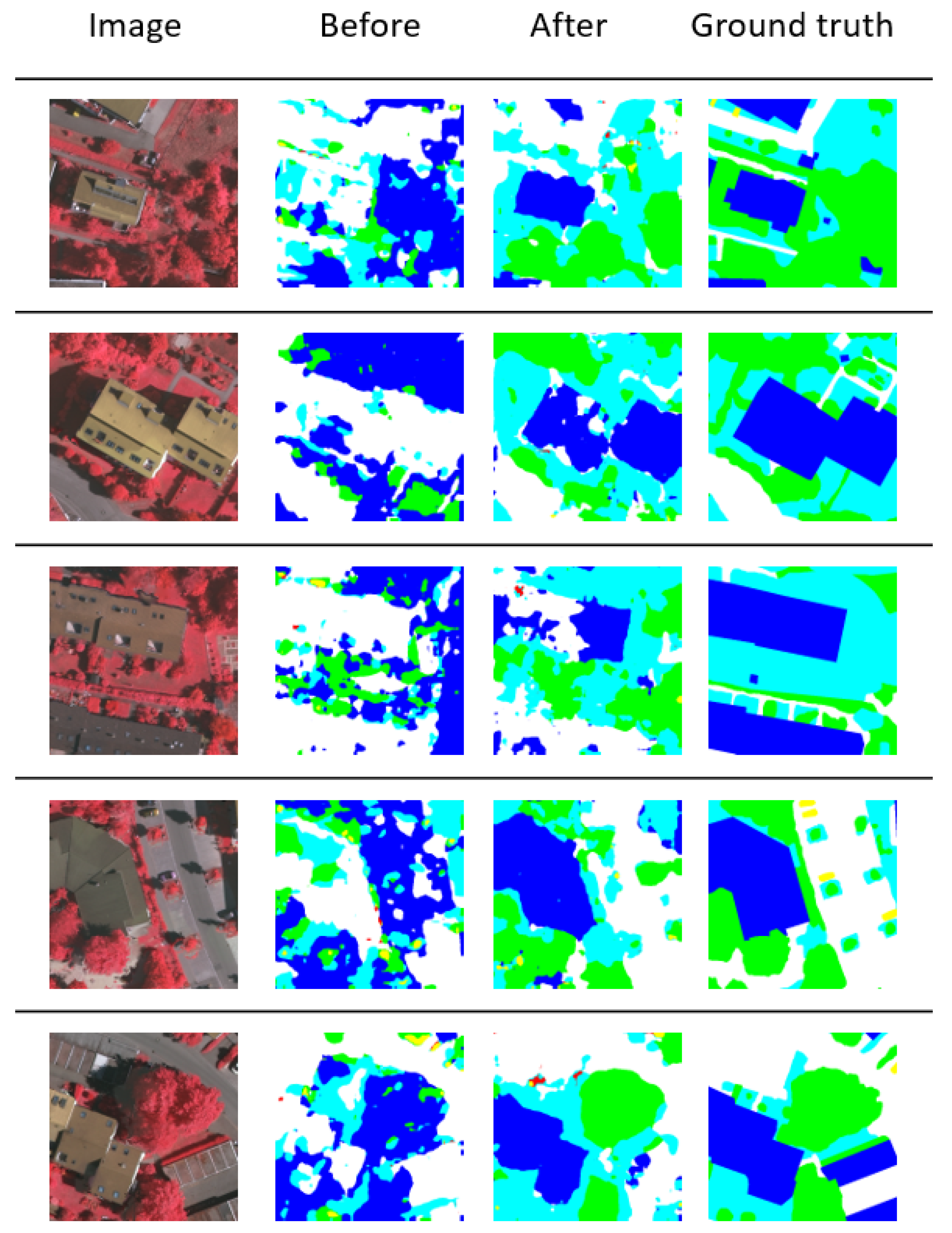
Once we finished the training of the first and the second GAN network, we apply Step 5 for segmentation of images from the target domain. We began by selecting the image we want to segment from the target domain (Vaihingen). Then we apply the first GAN network to translate this image to the label domain. The corresponding semantic label image will be passed into the second GAN network to generate the corresponding image in the source domain (Potsdam). The semantic segmentation model already trained on the source domain will be more able to segment this generated image because it is in the same domain it was trained on.

5.2.6. Discussion

The results of segmentation are always better using the generated image than the original one. Figure 11 shows the result of segmentation of some selected images from the target domain before and after application of our proposed algorithm. We can see clearly that our algorithm improves the quality of segmentation without needing too much data. The results in Figure 11 are generated using first GAN network trained only on 23 labeled images of size 512 512 from the target domain.
The improvement in segmentation accuracy increases with the number of labeled images picked out from the target domain. We tested different trainings of the GAN 1 model using 1, 3, 12, 23, 47, 94 and 188 labeled images from the target domain.
To select the source dataset from Vaihingen and Potsdam, we applied our algorithm twice. The first is done using Potsdam as source and Vaihingen as target, results are shown in Table 3. The second is done using Vaihingen as source and Potsdam as target, results are shown in Table 4. Both tables show the improvement made by the algorithm in segmentation accuracy, precision, sensitivity, dice coefficient and IoU for the different numbers of sampled images from the target domain.
As illustrated in Table 3 and Table 4, the algorithm efficiency is far better if we select Potsdam as the source. For similar number of labeled images (188 images in first case and 192 images in second case), improvement in average accuracy is 0.243 in first case and 0.026 in the second case. In fact, Potsdam dataset is far larger than Vaihingen dataset (3800 images in Potsdam and 459 images in Vaihingen). Training the segmentation model on a large dataset helps to better capture the global patterns of the data. Then, our algorithm will be more efficient in minimizing the domain shift that exists between the source and the target. This can be seen when selecting Potsdam as source in Table 3. If the source dataset is small, the segmentation model will be less able to learn the global patterns of the data. In this case, our algorithm will not be able to treat efficiently the domain shift. This can be seen when selecting Vaihingen as source a in Table 4. Hence, our algorithm works more efficiently if the source dataset is large enough to make the segmentation model capture the global patterns of the data.
As shown in Table 3, without our algorithm, the total accuracy was 34.5%. Using only 1 labeled images, accuracy increases to 36.8%. The more labeled images are added, the more the accuracy increases until reaching 58.8% for 188 labeled images from the target domain. 188 images represents only 4.9% of the images that was needed to train the segmentation model on the source dataset (3800 images of size 512 × 512 which proves the data efficiency of our algorithm. Figure 12, Figure 13, Figure 14, Figure 15 and Figure 16 respectively display the curves of accuracy, precision, sensitivity, F1 score and IoU for different numbers of sampled images from the target domain.
We deduced from the above curves that our algorithm increased the segmentation metrics by a significant margin, which explains the visible amelioration of the segmented map shown in Figure 11.
To judge the global efficiency of our algorithm, we compared it with two other domain adaptation algorithms. The first is FCNs in the wild [32]. It is a domain adaptation algorithm applied in general semantic segmentation. The second is the unsupervised algorithm introduced by Benjdira et al. [4]. It was designed specifically for domain adaptation in semantic segmentation of aerial imagery. We provided in Table 5 the comparison of average accuracy, dice coefficient (F1 score) and IoU in the task of domain adaptation from Potsdam to Vaihingen.
As shown in Table 5, our algorithm outperforms the other two algorithms in all measures. As a conclusion, the final user can choose between the unsupervised approach introduced by Benjdira et al. [4] and the current supervised approach. If the user does not want to invest time in labeling and wants a medium accuracy, he can choose the unsupervised approach. If he cares most about the accuracy, he can use the supervised approach presented in this paper. The choice will be a tradeoff between the labeling cost and the accuracy of domain adaptation.
Going deeper in the analysis of our algorithm, we studied its effect on the improvement of the segmentation accuracy for every class apart. Table 6 shows the improvement noted in each class for different numbers of sampled images. Moreover, we can validate that for every class, the more the size of labeled images increases, the more the segmentation accuracy is improved. This has some limited exceptions with some local decrease in the accuracy but did not affect the global improvement behavior. Only one class, the clutter background, knows a small decrease in accuracy and this is because there is no specific pattern to be learned for this class. It represents all the components that cannot be included within the other five classes, and the small number of samples is not sufficient for the first GAN network to capture the different patterns existing for this class. On the other side, classes Trees, Low vegetation and Building know a significant increase of accuracy by a margin of 47.7%, 21.9% and 31.6%, respectively. This is because the picked samples from the target domain were sufficient for the first GAN network to learn most of the patterns that exist for the class.
Figure 17 shows the curves of improvement of segmentation accuracy for every class for different sizes of the labeled images from the target domain.
Concerning the domain shift analysis of our algorithm, we note that it has no practical effect on classes that are not subject to domain shift (like class Impervious Surfaces and class Cars). In fact, our algorithm made an improvement of 0.8% for the class Car and 10.2% for the class Impervious Surfaces. On the other side, if the sensor domain shift factor is high on the class (See Table 2), the algorithm improves remarkably the segmentation accuracy. The improvement becomes smaller if it is combined with a high effect of other factors. For example, the class Trees and Buildings have a high effect of sensor variation factor and respectively medium and low effects of the class representation factor. The improvement is then 47.7% and 31.6%, respectively. We conclude, then, the efficiency of our algorithm in treating these cases of domain shift factors. On the other side, classes Low vegetation and clutter have a high effect of the sensor variation factor and a high effect of the class representation factor (the effect is much higher in the clutter class). The improvement is respectively 21.9% and −4.2%. We can conclude that the high effect of other domain shift factors reduces the impact of our algorithm, however, small to medium domain shift factors could be mitigated due to the supervision made by the labeled images. If the class patterns are presented in the labeled images (example: class Tree), the domain shift could be mitigated at a good degree. If the class patterns are so diversified and could not be provided in the small set of labeled images (example: class clutter background), the domain shift will be mitigated proportionally. This can be considered to be a limitation to our data-efficient approach. Hence, our algorithm is very efficient in treating the sensor variation factor. Concerning the class representation factor, our algorithm will be efficient in cases the effect is low to medium and most of the class patterns are provided within the labeled dataset.

6. Conclusions

In this study, we proposed a data-efficient supervised approach for domain adaptation in the context of semantic segmentation of aerial imagery. The algorithm is based on two GAN networks to translate images from the target to the source domain. This translation needs the provision of a small set of labeled images from the target domain. The method improves the segmentation accuracy by a margin up to 24% providing only 4.9% of the labeled data needed to train the segmentation model on the source dataset. Our method is confirmed to be efficient in treating the domain shift resulting from the sensor variation factor. It is also efficient in treating low to medium degrees of class representation factor if most of the class patterns are provided within the labeled data. Our work confirms the potential of GANs in aerial imagery analysis. Nevertheless, our algorithm should be combined with a solution to treat cases where we have high degree of class representation factor. Also, we should provide a remedy for cases where the class patterns are so diversified that they cannot be provided in the sampled images from the target domain. This can be solved using a semi-supervised approach to alleviate the manual work needed to label data.

Author Contributions

B.B. and A.A. designed the method. A.A. implemented the method. B.B. wrote the paper. A.K. and K.O. contributed to the supervision of the work. All authors have read and agreed to the published version of the manuscript.

Funding

This research was funded by Prince Sultan University.

Acknowledgments

This work is supported by Robotics and Internet of Things Lab (RIOTU), Prince Sultan University.

Conflicts of Interest

The authors declare no conflict of interest.

References

  1. Alhichri, H.; Jdira, B.B.; Alajlan, N. Multiple Object Scene Description for the Visually Impaired Using Pre-trained Convolutional Neural Networks. In Proceedings of the International Conference on Image Analysis and Recognition, Póvoa de Varzim, Portugal, 13–15 July 2016; Springer: Berlin/Heidelberg, Germany, 2016; pp. 290–295. [Google Scholar]
  2. Benjdira, B.; Khursheed, T.; Koubaa, A.; Ammar, A.; Ouni, K. Car Detection using Unmanned Aerial Vehicles: Comparison between Faster R-CNN and YOLOv3. In Proceedings of the 2019 1st International Conference on Unmanned Vehicle Systems-Oman (UVS), Muscat, Oman, 5–7 February 2019; IEEE: Piscataway, NJ, USA, 2019; pp. 1–6. [Google Scholar]
  3. Al Rahhal, M.M.; Bazi, Y.; Al Zuair, M.; Othman, E.; BenJdira, B. Convolutional neural networks for electrocardiogram classification. J. Med Biol. Eng. 2018, 38, 1014–1025. [Google Scholar] [CrossRef]
  4. Benjdira, B.; Bazi, Y.; Koubaa, A.; Ouni, K. Unsupervised Domain Adaptation Using Generative Adversarial Networks for Semantic Segmentation of Aerial Images. Remote. Sens. 2019, 11, 1369. [Google Scholar] [CrossRef] [Green Version]
  5. Ammour, N.; Alhichri, H.; Bazi, Y.; Benjdira, B.; Alajlan, N.; Zuair, M. Deep learning approach for car detection in UAV imagery. Remote. Sens. 2017, 9, 312. [Google Scholar] [CrossRef] [Green Version]
  6. Singh, V.K.; Rashwan, H.A.; Romani, S.; Akram, F.; Pandey, N.; Sarker, M.M.K.; Saleh, A.; Arenas, M.; Arquez, M.; Puig, D.; et al. Breast tumor segmentation and shape classification in mammograms using generative adversarial and convolutional neural network. Expert Syst. Appl. 2019, 139, 112855. [Google Scholar] [CrossRef]
  7. Ammar, A.; Koubaa, A.; Ahmed, M.; Saad, A. Aerial Images Processing for Car Detection using Convolutional Neural Networks: Comparison between Faster R-CNN and YoloV3. arXiv 2019, arXiv:1910.07234. [Google Scholar]
  8. Badrinarayanan, V.; Kendall, A.; Cipolla, R. SegNet: A Deep Convolutional Encoder-Decoder Architecture for Image Segmentation. IEEE Trans. Pattern Anal. Mach. Intell. 2017, 39, 2481–2495. [Google Scholar] [CrossRef]
  9. Zhao, H.; Shi, J.; Qi, X.; Wang, X.; Jia, J. Pyramid Scene Parsing Network. In Proceedings of the 2017 IEEE Conference on Computer Vision and Pattern Recognition (CVPR), Honolulu, HI, USA, 21–26 July 2017. [Google Scholar] [CrossRef] [Green Version]
  10. Ronneberger, O.; Fischer, P.; Brox, T. U-net: Convolutional networks for biomedical image segmentation. In Proceedings of the International Conference on Medical Image Computing and Computer-Assisted Intervention, Munich, Germany, 5–9 October 2015; Springer: Berlin/Heidelberg, Germany, 2015; pp. 234–241. [Google Scholar]
  11. Chen, L.C.; Papandreou, G.; Kokkinos, I.; Murphy, K.; Yuille, A.L. Deeplab: Semantic image segmentation with deep convolutional nets, atrous convolution, and fully connected crfs. IEEE Trans. Pattern Anal. Mach. Intell. 2018, 40, 834–848. [Google Scholar] [CrossRef]
  12. Dong, L.Y.; Sui, P.; Sun, P.; Li, Y.L. Novel naive Bayes classification algorithm based on semi-supervised learning. Jilin Daxue Xuebao (Gongxueban)/J. Jilin Univ. (Eng. Technol. Ed. 2016, 46, 884–889. [Google Scholar] [CrossRef]
  13. Cordts, M.; Omran, M.; Ramos, S.; Rehfeld, T.; Enzweiler, M.; Benenson, R.; Franke, U.; Roth, S.; Schiele, B. The cityscapes dataset for semantic urban scene understanding. In Proceedings of the IEEE conference on computer vision and pattern recognition, Las Vegas, NV, USA, 27–30 June 2016; pp. 3213–3223. [Google Scholar]
  14. Sun, P.; Brown, C.; Beschastnikh, I.; Stolee, K.T. Mining Specifications from Documentation using a Crowd. In Proceedings of the 2019 IEEE 26th International Conference on Software Analysis, Evolution and Reengineering (SANER), Hangzhou, China, 24–27 February 2019; pp. 275–286. [Google Scholar]
  15. Tzeng, E.; Hoffman, J.; Darrell, T.; Saenko, K. Simultaneous deep transfer across domains and tasks. In Proceedings of the IEEE International Conference on Computer Vision, Santiago, Chile, 7–13 December 2015; pp. 4068–4076. [Google Scholar]
  16. Long, M.; Cao, Y.; Wang, J.; Jordan, M.I. Learning transferable features with deep adaptation networks. arXiv 2015, arXiv:1502.02791. [Google Scholar]
  17. Tzeng, E.; Hoffman, J.; Saenko, K.; Darrell, T. Adversarial discriminative domain adaptation. In Proceedings of the Computer Vision and Pattern Recognition (CVPR), Honolulu, HI, USA, 21–26 July 2017; Volume 1, p. 4. [Google Scholar]
  18. Luo, Z.; Zou, Y.; Hoffman, J.; Fei-Fei, L.F. Label efficient learning of transferable representations acrosss domains and tasks. In Proceedings of the Advances in Neural Information Processing Systems, Long Beach, CA, USA, 4–9 December 2017; pp. 165–177. [Google Scholar]
  19. Goodfellow, I.; Pouget-Abadie, J.; Mirza, M.; Xu, B.; Warde-Farley, D.; Ozair, S.; Courville, A.; Bengio, Y. Generative adversarial nets. In Proceedings of the Advances in Neural Information Processing Systems, Montreal, QC, Canada, 8–13 December 2014; pp. 2672–2680. [Google Scholar]
  20. Isola, P.; Zhu, J.Y.; Zhou, T.; Efros, A.A. Image-to-Image Translation with Conditional Adversarial Networks. In Proceedings of the 2017 IEEE Conference on Computer Vision and Pattern Recognition (CVPR), Honolulu, HI, USA, 21–26 July 2017. [Google Scholar] [CrossRef] [Green Version]
  21. Patel, V.M.; Gopalan, R.; Li, R.; Chellappa, R. Visual Domain Adaptation: A survey of recent advances. IEEE Signal Process. Mag. 2015, 32, 53–69. [Google Scholar] [CrossRef]
  22. Saenko, K.; Kulis, B.; Fritz, M.; Darrell, T. Adapting visual category models to new domains. In Proceedings of the European Conference on Computer Vision, Heraklion, Crete, Greece, 5–11 September 2010; Springer: Berlin/Heidelberg, Germany, 2010; pp. 213–226. [Google Scholar]
  23. Ganin, Y.; Ustinova, E.; Ajakan, H.; Germain, P.; Larochelle, H.; Laviolette, F.; Marchand, M.; Lempitsky, V. Domain-adversarial training of neural networks. J. Mach. Learn. Res. 2016, 17, 2096–2030. [Google Scholar]
  24. Ganin, Y.; Lempitsky, V. Unsupervised domain adaptation by backpropagation. arXiv 2014, arXiv:1409.7495. [Google Scholar]
  25. Bousmalis, K.; Silberman, N.; Dohan, D.; Erhan, D.; Krishnan, D. Unsupervised pixel-level domain adaptation with generative adversarial networks. In Proceedings of the IEEE Conference on Computer Vision and Pattern Recognition, Honolulu, HI, USA, 21–26 July 2017; pp. 3722–3731. [Google Scholar]
  26. Hoffman, J.; Tzeng, E.; Park, T.; Zhu, J.Y.; Isola, P.; Saenko, K.; Efros, A.A.; Darrell, T. Cycada: Cycle-consistent adversarial domain adaptation. arXiv 2017, arXiv:1711.03213. [Google Scholar]
  27. Ros, G.; Sellart, L.; Materzynska, J.; Vazquez, D.; Lopez, A.M. The synthia dataset: A large collection of synthetic images for semantic segmentation of urban scenes. In Proceedings of the IEEE conference on Computer Vision and Pattern Recognition, Las Vegas, NV, USA, 27–30 June 2016; pp. 3234–3243. [Google Scholar]
  28. Vazquez, D.; Lopez, A.M.; Marin, J.; Ponsa, D.; Geronimo, D. Virtual and real world adaptation for pedestrian detection. IEEE Trans. Pattern Anal. Mach. Intell. 2014, 36, 797–809. [Google Scholar] [CrossRef] [PubMed]
  29. Peng, X.; Saenko, K. Synthetic to real adaptation with generative correlation alignment networks. In Proceedings of the 2018 IEEE Winter Conference on Applications of Computer Vision (WACV), Lake Tahoe, NV, USA, 12–15 March 2018; pp. 1982–1991. [Google Scholar]
  30. Shrivastava, A.; Pfister, T.; Tuzel, O.; Susskind, J.; Wang, W.; Webb, R. Learning from simulated and unsupervised images through adversarial training. In Proceedings of the IEEE Conference on Computer Vision and Pattern Recognition, Honolulu, HI, USA, 21–26 July 2017; pp. 2107–2116. [Google Scholar]
  31. Shafaei, A.; Little, J.J.; Schmidt, M. Play and learn: Using video games to train computer vision models. arXiv 2016, arXiv:1608.01745. [Google Scholar]
  32. Hoffman, J.; Wang, D.; Yu, F.; Darrell, T. Fcns in the wild: Pixel-level adversarial and constraint-based adaptation. arXiv 2016, arXiv:1612.02649. [Google Scholar]
  33. Zhang, Y.; David, P.; Gong, B. Curriculum domain adaptation for semantic segmentation of urban scenes. In Proceedings of the IEEE International Conference on Computer Vision, Venice, Italy, 22–29 October 2017; pp. 2020–2030. [Google Scholar]
  34. Sankaranarayanan, S.; Balaji, Y.; Jain, A.; Lim, S.N.; Chellappa, R. Unsupervised domain adaptation for semantic segmentation with gans. arXiv 2017, arXiv:1711.06969. [Google Scholar]
  35. Tsai, Y.H.; Hung, W.C.; Schulter, S.; Sohn, K.; Yang, M.H.; Chandraker, M. Learning to adapt structured output space for semantic segmentation. In Proceedings of the IEEE Conference on Computer Vision and Pattern Recognition, Salt Lake City, UT, USA, 18–22 June 2018; pp. 7472–7481. [Google Scholar]
  36. Huang, H.; Huang, Q.; Krahenbuhl, P. Domain transfer through deep activation matching. In Proceedings of the European Conference on Computer Vision (ECCV), Munich, Germany, 8–14 September 2018; pp. 590–605. [Google Scholar]
  37. Tasar, O.; Happy, S.L.; Tarabalka, Y.; Alliez, P. ColorMapGAN: Unsupervised Domain Adaptation for Semantic Segmentation Using Color Mapping Generative Adversarial Networks. arXiv 2019, arXiv:1907.12859. [Google Scholar]
  38. Fang, B.; Kou, R.; Pan, L.; Chen, P. Category-Sensitive Domain Adaptation for Land Cover Mapping in Aerial Scenes. Remote. Sens. 2019, 11, 2631. [Google Scholar] [CrossRef] [Green Version]
  39. Gerke, M. Use of the Stair Vision Library Within the ISPRS 2D Semantic Labeling Benchmark (Vaihingen); University of Twente: Enschede, The Nerthands, 2014. [Google Scholar]
  40. Oliehoek, F.A.; Savani, R.; Gallego, J.; van der Pol, E.; Gross, R. Beyond Local Nash Equilibria for Adversarial Networks. arXiv 2018, arXiv:1806.07268. [Google Scholar]
  41. Goodfellow, I.J. NIPS 2016 Tutorial: Generative Adversarial Networks. arXiv 2016, arXiv:1701.00160. [Google Scholar]
  42. Liu, M.Y.; Breuel, T.; Kautz, J. Unsupervised Image-to-Image Translation Networks. In Proceedings of the Advances in Neural Information Processing Systems 30 (NIPS 2017), Long Beach, NV, USA, 4–9 December 2017. [Google Scholar]
  43. Zhu, J.Y.; Zhang, R.; Pathak, D.; Darrell, T.; Efros, A.A.; Wang, O.; Shechtman, E. Toward Multimodal Image-to-Image Translation. In Proceedings of the Advances in Neural Information Processing Systems 30 (NIPS 2017), Long Beach, NV, USA, 4–9 December 2017. [Google Scholar]
  44. Yi, Z.; Zhang, H.; Tan, P.; Gong, M. DualGAN: Unsupervised Dual Learning for Image-to-Image Translation. In Proceedings of the 2017 IEEE International Conference on Computer Vision (ICCV), Venice, Italy, 22–29 October 2017; pp. 2868–2876. [Google Scholar]
  45. Zhu, J.Y.; Park, T.; Isola, P.; Efros, A.A. Unpaired Image-to-Image Translation Using Cycle-Consistent Adversarial Networks. In Proceedings of the 2017 IEEE International Conference on Computer Vision (ICCV), Venice, Italy, 22–29 October 2017. [Google Scholar] [CrossRef] [Green Version]
  46. Xu, B.; Wang, N.; Chen, T.; Li, M. Empirical Evaluation of Rectified Activations in Convolutional Network. arXiv 2015, arXiv:1505.00853. [Google Scholar]
  47. Ioffe, S.; Szegedy, C. Batch Normalization: Accelerating Deep Network Training by Reducing Internal Covariate Shift. arXiv 2015, arXiv:1502.03167. [Google Scholar]
  48. Srivastava, N.; Hinton, G.E.; Krizhevsky, A.; Sutskever, I.; Salakhutdinov, R.R. Dropout: A simple way to prevent neural networks from overfitting. J. Mach. Learn. Res. 2014, 15, 1929–1958. [Google Scholar]
  49. Mirza, M.; Osindero, S. Conditional Generative Adversarial Nets. arXiv 2014, arXiv:1411.1784. [Google Scholar]
  50. Yu, C.; Wang, J.; Peng, C.; Gao, C.; Yu, G.; Sang, N. BiSeNet: Bilateral Segmentation Network for Real-Time Semantic Segmentation. In Proceedings of the European Conference on Computer Vision, Lecture Notes in Computer Science, Munich, Germany, 8–14 September 2018; pp. 334–349. [Google Scholar] [CrossRef] [Green Version]
  51. Real-Time Semantic Segmentation on Cityscapes. Available online: https://paperswithcode.com/sota/real-time-semantic-segmentation-cityscap (accessed on 28 March 2019).
  52. Semantic Segmentation Suite. Available online: https://github.com/GeorgeSeif/Semantic-Segmentation-Suite (accessed on 28 March 2019).
  53. Abadi, M.; Barham, P.; Chen, J.; Chen, Z.; Davis, A.; Dean, J.; Devin, M.; Ghemawat, S.; Irving, G.; Isard, M.; et al. TensorFlow: A system for large-scale machine learning. In Proceedings of the 12th USENIX Symposium on Operating Systems Design and Implementation (OSDI 16), Savannah, GA, USA, 2–4 November 2016; pp. 265–283. [Google Scholar]
  54. He, K.; Zhang, X.; Ren, S.; Sun, J. Deep Residual Learning for Image Recognition. In Proceedings of the 2016 IEEE Conference on Computer Vision and Pattern Recognition (CVPR), Las Vegas, NV, USA, 26 June–1 July 2016. [Google Scholar] [CrossRef] [Green Version]
  55. Kingma, D.P.; Ba, J. Adam: A Method for Stochastic Optimization. arXiv 2014, arXiv:1412.6980. [Google Scholar]
Figure 1. Cross-domains semantic segmentation of aerial imagery.
Applsci 10 01092 g001
Figure 2. Standard architecture of the GAN.
Applsci 10 01092 g002
Figure 3. The GAN architecture.
Applsci 10 01092 g003
Figure 4. The architecture of the first GAN network: (a) the generator and (b) the discriminator.
Applsci 10 01092 g004
Figure 5. Flowchart of the domain adaptation algorithm.
Applsci 10 01092 g005
Figure 6. Image samples from Vaihingen and Potsdam ISPRS datasets.
Applsci 10 01092 g006
Figure 7. The Architecture of BiSeNet (Bilateral Segmentation Network).
Applsci 10 01092 g007
Figure 8. Progress of segmentation accuracy of BiseNet trained on Potsdam.
Applsci 10 01092 g008
Figure 9. Curve of the loss during the training of BiseNet on Potsdam dataset.
Applsci 10 01092 g009
Figure 10. Translation of images from the label domain to the source domain using the second GAN network.
Applsci 10 01092 g010
Figure 11. Segmentation of images from the target domain before and after application of our proposed algorithm.
Applsci 10 01092 g011
Figure 12. Segmentation accuracy for different numbers of sampled images from the target domain.
Applsci 10 01092 g012
Figure 13. Segmentation precision for different numbers of sampled images from the target domain.
Applsci 10 01092 g013
Figure 14. Segmentation sensitivity for different numbers of sampled images from the target domain.
Applsci 10 01092 g014
Figure 15. Segmentation dice coefficient for different numbers of sampled images from the target domain.
Applsci 10 01092 g015
Figure 16. Segmentation IoU for different numbers of sampled from the target domain.
Applsci 10 01092 g016
Figure 17. Segmentation accuracy per class for different sizes of the labeled images from the target domain.
Applsci 10 01092 g017
Table 1. The distribution of pixels among categories.
CategoryPotsdamVaihingen
Buildings28.2%26.9%
Impervious Surfaces29.9%29.3%
Low vegetation20.9%19.4%
Trees14.4%22.4%
Clutter4.8%0.7%
Cars1.7%1.3%
Table 2. Domain shift analysis when passing from Potsdam to Vaihingen.
Domain Shift FactorResolutionSensorClass Representation
Treeslowhighmedium
Carslowlowlow
Clutterlowhighhigh
Impervious Surfaceslowlowlow
Buildingslowhighlow
Low vegetationlowhighhigh
Table 3. Segmentation Accuracy, Precision, Sensitivity, Dice Coefficient and IoU score for different numbers of sampled images from the target domain (Potsdam as source and Vaihingen as target).
Number of Images from TargetAverage AccuracyPrecisionSensitivityDice CoefIoU
00.3450.3450.3450.3160.175
10.3680.4450.3680.3600.176
30.4220.4700.4220.4040.214
120.4740.5130.4740.4550.253
230.5070.5410.5070.4880.281
470.5240.5590.5240.5050.297
940.5590.5910.5590.5430.327
1880.5880.6250.5880.5720.349
Table 4. Segmentation Accuracy, Precision, Sensitivity, Dice Coefficient and IoU score for different numbers of sampled images from the target domain (Vaihingen as source and Potsdam as target).
Number of Images from TargetAverage AccuracyPrecisionSensitivityDice CoefIoU
00.3340.3350.3340.2880.169
1920.3630.3650.3630.3180.179
Table 5. Segmentation Accuracy, Dice Coefficient and IoU score for different domain adaptation algorithms (Potsdam as source and Vaihingen as target).
MethodAverage AccuracyDice CoefIoU
Without Domain Adaptation0.3450.3160.175
FCNs in the wild0.4860.4130.309
Unsupervised Method in [4]0.5200.4900.300
Ours (188 images)0.5880.5720.349
Table 6. Improvement of per-class accuracy for different numbers of sampled images from the target domain.
Nb of ImagesImp. Surf.BuildingLow Veget.TreeCarClutter Backgr.
00.5830.2270.3830.0620.4000.935
10.5910.2650.3680.3110.3230.893
30.4770.3030.5530.4170.3230.893
120.5380.4390.5590.4020.3250.894
230.6020.4670.5730.4210.3380.894
470.6050.4160.5750.5200.3850.893
940.6340.4630.6180.5090.4050.893
1880.6850.5430.6020.5390.4080.893

