Abstract
The grounded electrical-source airborne transient electromagnetic (GREATEM) system is widely used in mineral exploration. Meanwhile, the induced polarization (IP) effect, which indicates the polarizability of the earth, is often found. In this paper, the Maxwell equations in the frequency domain are transformed into fictitious wave domain, where Maxwell equations are solved by the time domain finite difference method. Then, an integral transformation method is used to convert the calculation results back to the time domain. A three-dimensional (3D) numerical simulation in a polarizable medium is presented. The accuracy of this method is proven by comparing it with the analytical solution and the existing method, and the calculation efficiency is increased five-fold. The simulation results show that the GREATEM system has a higher response amplitude in the conductive region, while IP effects cannot be identified in the conductive area. The GREATEM system has a higher response amplitude in the low-resistance region, but IP effects cannot be identified in the low-resistance area, and the detection of IP effects is more suitable for the high-resistance area. Therefore, it is necessary to improve the detection ability of the GREATEM system in the low-resistance area.
1. Introduction
Electromagnetic technology has a wide range of applications in various fields. Nasim (2019) proposed a metamaterial platform for solving integral equations using a monochromatic electromagnetic field [1]. The application of electromagnetic technology in medical diagnosis equipment realizes the measurement of blood glucose and the detection of cancer stage [2,3]. In addition, it is necessary to consider electromagnetic fields in plasma electronics [4,5].
Here, we apply electromagnetic technology to geophysics. Grounded electrical-source airborne transient electromagnetic (GREATEM) is a useful detection geophysical method where the transmitter is set on the ground and the receiver is installed on the aircraft [6]. Combining the ground and airborne electromagnetic systems, GREATEM has the advantages of large detection depth, high resolution, wide range, and fast speed. In particular, it has unique superiority in mountains, forest-covered areas, swamps, and other special areas [7,8]. Ji (2013) used an airship as the carrier and the two-dimensional finite difference method to calculate the time-domain GREATEM response with a long wire source [9]. Ren (2017) investigated a three-dimensional time-domain airborne electromagnetic model based on the finite volume method, and then used the strategy of separating the primary field from the secondary field, which significantly saved on calculation time [10]. For airborne transient electromagnetic measurement, a three-dimensional forward simulation method which considered attitude change was proposed, and the electromagnetic response of a shallow surface was analyzed in Reference [11]. Later, the spectral element method (SE) was used to carry out three-dimensional modeling of GREATEM, effectively improving the modeling accuracy [12].
To interpret GREATEM, researchers often make the assumption that the earth is just conductive or resistive. However, there is an induced polarization (IP)effect in the earth, which is usually reflected as a reverse signal. The existence of the IP effect has a great impact on the electromagnetic response [13,14]. The IP effect is related to conductivity and frequency, and its dispersion characteristics can be expressed by the Debye model and the Cole–Cole model [15,16]. At present, numerical simulations of the polarization effect are mainly conducted in the frequency domain. Most of the early studies simulated the IP effect by converting the electromagnetic field from the frequency domain to the time domain [17,18]. Unfortunately, when broadband frequency content is considered, the methods are not so efficient [19]. In order to simulate the IP effect in the time domain, Kang (2015) proposed a method to generate a three-dimensional pseudo charge distribution using airborne time-domain electromagnetic data and effectively extracted the polarization signal [20]. Wu (2017) used the FDTD (finite difference time-domain) method to simulate the IP effect with a small loop source [21]. Commer (2017) expanded the finite difference time-domain scheme, modeled and analyzed the IP effect, and developed a simple calculation of the Cole–Cole model [22].
However, three-dimensional (3D) numerical simulations of IP effects based on FDTD require a high computation load, when including the air layer. In addition, it is difficult to calculate the source in the FDTD method; thus, the upward continuation method is often used to avoid directly loading the emission source. Mittet (2010) put forward the theory of wave field transformation and successfully applied it to marine CSEM (controllable source electromagnetic method), increasing the calculation efficiency by nearly 10-fold [23]. Mittet (2018) used the least squares fitting method to calculate the IP response of sea water in the fictitious wave field [24]. Ji (2017) improved the emission source, applied the wave field transformation method to the ground transient electromagnetic simulation, and realized a three-dimensional transient electromagnetic numerical simulation including the air layer [25]. However, it did not consider the IP effect of the earth. Therefore, here, we perform the wave field transformation in GREATEM, and we realize a three-dimensional numerical simulation in polarizable media using the Cole–Cole model. In addition, the computing efficiency is also improved.
The wave field transformation method is proposed for the grounded electrical-source airborne transient electromagnetic system in this paper. The Maxwell equations in the real diffusion field are transformed into the fictitious wave field by using the transformation relationship between the diffusion field and fictitious wave field. The fractional order Cole–Cole model is introduced into the fictitious wave field, and the Maxwell equations with the Cole–Cole model are solved using the finite difference time-domain method. Finally, an integral transformation method is used to transform the calculation results back to the real diffusion field. In the case of including polarized media, the two-field numerical simulation of the induction field and polarization field is realized. In addition, the computing efficiency is also improved.
2. Wave Field Transformation Theory Based on Fractional-Order Cole–Cole Model
2.1. Transformation from Real Diffusion Field to Fictitious Wave Field
The Maxwell equation in the frequency domain of the real diffusion field is written as follows:
where E and H are the electric and magnetic fields in the real diffusion field, respectively, J denotes the current density, and K denotes the magnetic current density. is the angular frequency, is permeability tensor, and σ is conductivity, while x is the direction.
The IP effect can be described by the Cole–Cole model [16].
where is the conductivity corresponding to infinite frequency, is the characteristic time constant, and c and are the frequency dependence and chargeability, respectively.
Applying Equation (3) to the frequency-domain Maxwell equation (Equation (1)), we can get
A fictitious dielectric constant is defined by the conductivity tensor (Mittet, 2010).
where is the scaling parameter, , and is the fictitious dielectric permittivity tensor. Substituting Equation (5) into Equation (4), we can get
Multiplying both sides of Equation (6) by gives
Equation (2) can be rewritten as
The relationship between the real diffusion field and fictitious wave field was given by Reference [23].
where is the scaling parameter, is the angular frequency in the fictitious wave field, and are the current and magnetic current densities in the fictitious wave field, and and are the electric and magnetic fields in the fictitious wave domain.
Using Equations (9)–(13), Equations (7) and (8) can be written in terms of fictitious wave fields.
Because the appropriate kernel used to decompose the spectra is closer to a Cole–Cole function with an exponent c of 0.5 [26], then
Assuming , the time-domain expressions (Equations (16) and (17)) can be obtained through inverse Fourier transform.
By combining Equations (18) and (19), the electric and magnetic field x-components can be found as
where
Equation (22) can be solved by iteration, as shown in Equation (23).
where , and the forward staggered time step is .
2.2. Electrical Source Loading in Fictitious Wave Field
As shown in Figure 1, Tx is the long wire source and Rx is the receiver. The fictitious emission source is only related to x- and y-components of the electric field, and the z-component is zero.
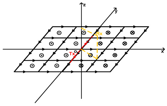
Figure 1.
Loading mode of fictitious wave field long wire source.
Here, the first-order Gaussian pulse is selected as the fictitious emitter, as shown in Equation (24).
where , is the maximum frequency in the fictitious wave field.
2.3. The Transformation from Fictitious Wave Field to Real Diffusion Field
It should be noted that the fictitious wave field is only used for the convenience of calculation, and it does not exist in reality. Therefore, we need to transform it back to the real diffusion field. The transformations are as follows [23]:
where is the total calculation time in the fictitious wave field, and is the sample time.
2.4. Loading Complex Frequency Shifted Perfectly Matched Layer (CFS-PML) in Fictitious Wave Field
Roden (2000) proposed CFS-PML (complex frequency shifted perfectly matched layer) boundary conditions, which significantly saved on memory [27]. The CFS-PML boundary conditions are introduced into the fictitious wave field to improve the absorption effect of the boundary on the low-frequency wave [28].
In x-components, Maxwell’s curl equations are as follows:
It should be noted that is the imaginary unit in Maxwell equations, and i, j, and k are the three direction vectors of the coordinate system. , , and are the coordinate stretching factors, , , and . By setting , , we can get the original stretched coordinate metrics, which is the PML boundary condition.
Taking as an example, and using Equations (29) and (30), we can get
Applying Laplace transform to (31) to the time domain, the iterative solution can be obtained.
On the boundary parameters, and , which depend on the relative positions of nodes and target areas, are not fixed, whereas and are two discrete variables.
where indicates the intersection of the boundary and the target area boundary, is the boundary thickness, and is the polynomial parameter.
3. Accuracy and Efficiency Verification of the Calculation Method
3.1. Half Space Model with IP Effect
In the field measurement with GREATEM, only the change of the underground secondary field is considered. In the process of numerical simulation, people usually divide the real space into two parts (air and ground), without considering the interface between the ground and air. Therefore, in the research process of this paper, the ground and the interface are not considered. In order to verify the effectiveness of this method, we design a half-space model incorporating the IP effect, as shown in Figure 2. Let the conductivity of the air layer , conductivity at the infinite frequency of the half-space model , chargeability , characteristic time constant , and frequency dependence . Tx represents the transmitter, Rx is the receiver, the horizontal distance between Tx and Rx (offset distance) is 300 m, and the flight altitude is h = 0 m. In Figure 3, the calculation results are compared with Reference [29]. We can see that the solution of the fictitious domain finite difference method (FW-FDTD) is in good agreement with that of the transformed frequency domain method. The average relative error of both methods is less than 10%.
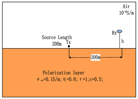
Figure 2.
The half-space model with induced polarization (IP) effect.
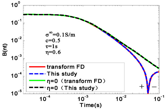
Figure 3.
The response curve of the half-space model.
When the earth contains the IP effects, the polarization parameters have great influence on the induced-polarization (IP) effects. In order to analyze the influence of polarization parameters on IP effects, we take the uniform half space model (Figure 2) as an example. Set the air layer conductivity , a 200-m-long wire source is selected as the transmitter, and the offset distance is r = 300 m. Furthermore, chargeability , conductivity at infinite frequency , frequency dependence , and flight altitude . The characteristic time constant is selected as , , and . The IP response under different characteristic time constants is calculated as shown in Figure 4. Other parameters remain unchanged. The characteristic time constant is set to , and . The conductivity at infinite frequency is , , and . The IP response under different conductivity is calculated as shown in Figure 5. Furthermore, , , and the chargeability is , , and . The response curves under different chargeability are calculated as shown in Figure 6.
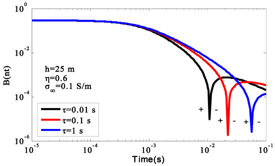
Figure 4.
Influence of characteristic time constant on IP effect.
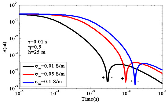
Figure 5.
Influence of conductivity at infinite frequency on IP effect.
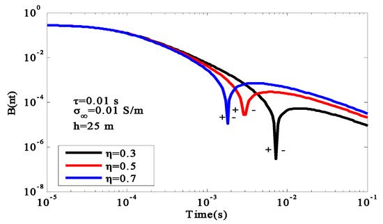
Figure 6.
Influence of chargeability on IP effect.
From Figure 4, Figure 5 and Figure 6, it can be seen that characteristic time constant, chargeability, and conductivity at infinite frequency affect the occurrence time of negative response, and all responses are monotonic. Compared with the conductivity at infinite frequency, the effect of characteristic time constant and chargeability on the IP response is lower, mainly in the late stage, and the change trend of the early induction field is basically the same. With the decrease in characteristic time constant, the time of minus response is gradually advanced. With the decrease in chargeability, the time of minus response is delayed. The conductivity at infinite frequency has a great influence on the IP effect. In addition to the minus response at the later stage, it also has a great influence on the early induction field. In the early stage, the response amplitude of the induction field increases gradually with the increase in conductivity at infinite frequency. In the later period, a smaller conductivity at infinite frequency results in the minus response appearing earlier.
3.2. Three-Dimensional Model
In addition, we calculated a three-dimensional model with a chargeable anomaly and compared the result with Reference [30]. The dimensions of the cell mesh were , and the minimum grid size was . The modeling volume was . The size of the chargeable anomaly was , while the distance from the top to the bottom of the chargeable anomaly was 40 m. The parameters of the Cole–Cole model were , , , and . The background conductivity was . A vertical point dipole emitter, which was located 30 m above the surface, was used, and the receiver and transmitter were at the same location. The calculation results are shown in Figure 7, from which it can been seen that the two IP effect curves were consistent. The relative error was less than 10%, which further verifies the correctness of the method.
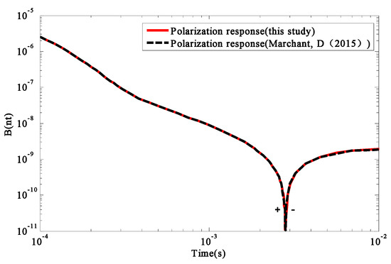
Figure 7.
Comparison of this study with that of Reference [29].
In terms of computation load, the iterations in the fictitious wave field are as follows:
where represents the number of iteration steps, is the maximum transceiver distance, and are the maximum and minimum conductivity, respectively, and is the minimum grid size. Using Equation (37), the number of iteration steps was 76,681. It should be noted that only one transmitter rather than an array was selected in this work. Compared with Reference [30], the calculation efficiency was improved by about five-fold.
4. Calculation Results of the Three-Dimensional Chargeable Body Model
The phenomenon of the inverse sign (IP effect) often appears in GREATEM. Most researchers focused on the influence of the IP parameters. However, in addition to the IP parameters, the system parameters of GREATEM also have an impact on the IP effect. In this section, we mainly analyze the effect of the system parameters, and we provide a theoretical basis for the field measurements.
4.1. Forward Modeling Results of 3D Chargeable Body
In order to analyze the influence of system parameters on the IP effect, we build a three-dimensional model with the consideration of a chargeable body, as shown in Figure 8. The ground conductivity was , the air layer conductivity was , Tx was the long wire source, the length was , Rx represents the receiving point, the height from the ground was , and the offset distance was . The dimensions of the chargeable body were , which was 100 m below the surface. The model parameters of the chargeable body were selected as follows: chargeability , frequency dependence , and characteristic time constant . The conductivities at infinite frequency were , , and . The calculation results are shown in Figure 9. The snapshots of the induced current system in the fictitious wave field are shown in Figure 10a,b.
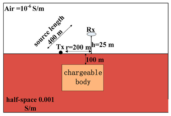
Figure 8.
Three-dimensional (3D) model with IP effect.
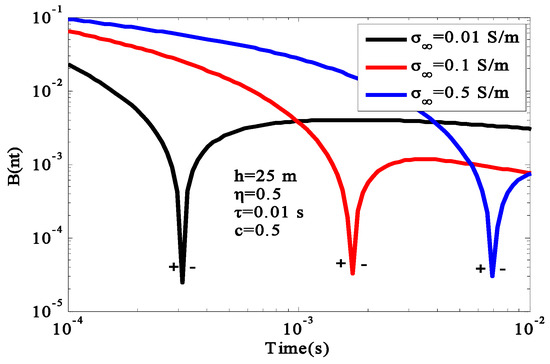
Figure 9.
Response curves under different conductivities.
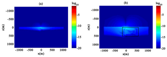
Figure 10.
The snapshots of the induced current system in the fictitious wave field (a) early time; (b) late time.
It can be seen from Figure 9 that, with the increase in conductivity at the infinite frequency, the attenuation of the early induction field gradually decreased, the attenuation of the late IP response gradually quickened, and the occurrence time of the inverse sign gradually delayed. This is because the influence of the induction field of the low-resistance body was greater than that of the high-resistance body. Therefore, the second field decayed slowly, and the negative response appeared later. Thus, the polarization phenomenon was more easily observed on the high-resistance body. The chargeable body position can be clearly observed from Figure 10, and the method of wave field transformation could effectively identify the polarizable body. Since we set the air layer as a finite high-resistance body, the conductivity was not zero, and the propagation of induced current in the air layer was not zero. In the fictitious wave field, due to the influence of the chargeable body, the propagation mode of the electromagnetic field changed, and it no longer propagated in the form of symmetry.
After setting , as well as the ground conductivity , , and , which are associated with high-, medium-, and low-resistance areas, the IP effects were calculated as shown in Figure 11.
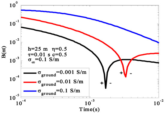
Figure 11.
IP effects under different background conductivities.
With the increase in ground conductivity, the amplitude of the early induction field and the late polarization field increased. In the high- and middle-resistance regions, the negative responses occurred at 1.7 ms and 3.3 ms. On the other hand, in the low-resistance region, the negative response could not be observed. When the negative value reached the minimum, the curve decayed approximately exponentially. The GREATEM had better resolution in the low-resistance region, but it is more suitable for the high-resistance region when measuring the IP effect.
4.2. The Influence of System Parameters on IP Response
In the field measurements of GREATEM, due to the influence of airflow and environment, the flight height was not a constant. Therefore, it was necessary to analyze the influence of flight altitude on the IP effect. We take the 3D model (Figure 8) as an example. The air layer conductivity was set to and the earth conductivity was set to , while the size of the chargeable body was . The model parameters of the chargeable body were as follows: chargeability , frequency dependence , characteristic time constant , conductivity at the infinite frequency , offset distance , and flight altitude , , , and . The induced polarization (IP) effect at different flight altitudes was calculated as depicted in Figure 12. In order to understand the influence of the parameters of GREATEM on the IP response, other parameters remained unchanged, while the flight height was set to h = 25 m, and the emission source length was , , and . The responses of different emission source lengths are shown in Figure 13. Taking and the offset distance , , and , the responses of different offsets are shown in Figure 14.
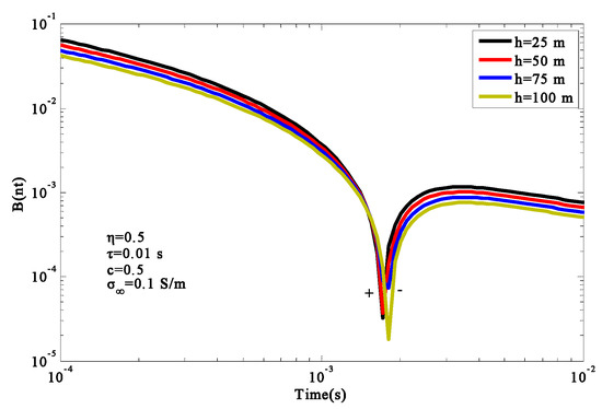
Figure 12.
IP effects at different flight altitudes.
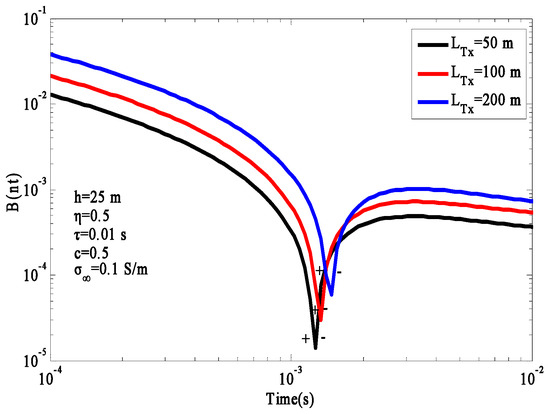
Figure 13.
The response curves under different emission source lengths.
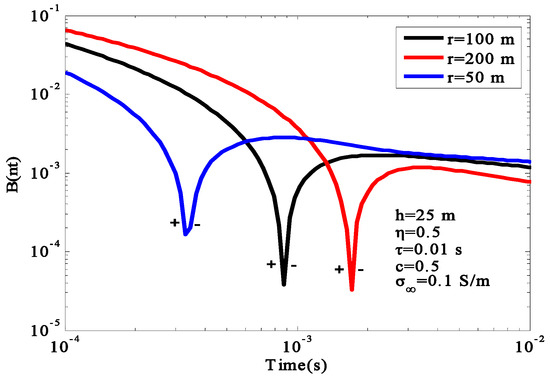
Figure 14.
The response curves under different offset distances.
Based on Figure 12, flight altitude mainly affected the amplitude of the response. The effect on the time of sign reversal was not obvious, and the sign reversal phenomenon was mainly concentrated in the range 1.5–2 ms. With the increase in flight altitude, the received electromagnetic response decreased gradually. It can be seen from Figure 13 that the length of the emission source mainly affected the amplitude of the response. The length of emission source increased gradually, and the amplitude of response increased gradually, which also shows that a longer emission source resulted in a higher resolution of the polarizable body. In Figure 14, with the decrease in offset distance, the time of the sign reversal appeared earlier, and the polarization response became easier to observe at a short offset distance.
Next, we set the air layer conductivity to and earth conductivity to . The size of the chargeable body was . The model parameters of the chargeable body were chosen as , , , , offset distance , emission source length , and flight altitude . The chargeable body was buried and below the surface. The response curves of the chargeable body at different depths are shown in Figure 15. Moreover, we changed the size of the chargeable body to and the chargeable body depth to , while keeping other parameters the same, and setting the distance from the left boundary of the chargeable body to the emission source as , , and . The response curves at different source positions are shown in Figure 16.
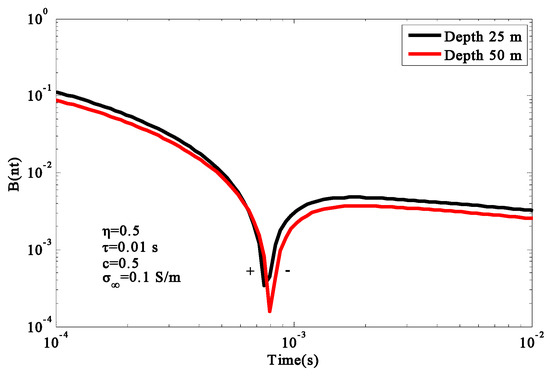
Figure 15.
The influence of chargeable body depth on response curve.
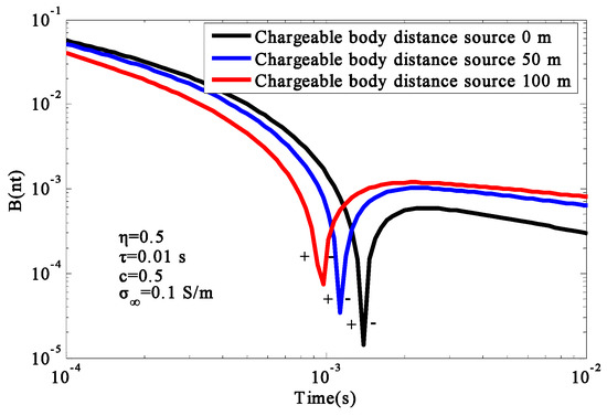
Figure 16.
The influence of different emitter locations on IP effect.
From Figure 15 and Figure 16, it can be seen that all the amplitudes decreased, while the depth of chargeable body increased. However, the time of the reversal sign did not change. In the early stage, as the distance between the emitter source and the chargeable body decreased, the amplitude of the induced field increased, the attenuation of the curve was delayed. In the later stage, the time of sign reversal appeared later when the distance between the emitter and the chargeable body decreased.
5. Conclusions
Three-dimensional numerical simulations are the basis of data interpretation and imaging. In this paper, a three-dimensional numerical simulation of underground polarized media was realized, which achieved simulation results closer to the actual mineral resources. In the actual measurement process with GREATEM, the geodetic model could be established using this method, and the optimal configuration structure of the equipment was obtained using the numerical simulation method. This not only provides the basis for the exploration of underground mineral resources, but also provides theoretical guidance for the design of detection instruments. Wave field transformation was proposed to calculate the response of the GREATEM system using the Cole–Cole model. The electromagnetic wave was absorbed by the boundary condition of CFS-PML in the fictitious wave field. Compared with the analytical solution and the transformed FD method, the relative error was less than 10%, satisfying the standard calculation requirements. Compared with the existing method, the calculation time was reduced five-fold. According to the simulations, the flight altitude, electrical source length, electrical source position, and the offset distance all affected the electromagnetic response monotonically. In the homogeneous half-space model, when the characteristic time constant () and conductivity at the infinite frequency () were too large, the negative response was likely overwhelmed by the noise; thus, the negative response could not be observed. Therefore, the occurrence time of the negative response could be enhanced by reducing the offset distance. Low-altitude flights can facilitate the recognition ability of the chargeable body, but they are often limited by geological conditions. The response of the GREATEM system had good recognition ability in the low-resistance area; however, the chargeable body could hardly be detected. Therefore, it is necessary to improve the detection accuracy of the GREATEM in low-resistance areas.
This paper realized a three-dimensional numerical simulation of polarized media based on the Cole–Cole model, and improved the calculation efficiency. However, in the actual measurement process, the underground medium is diverse. It is not comprehensive to only use the Cole–Cole model to describe the characteristics of polarized medium; the existence of the GEMTIP model in particular is a major problem in the field of geophysics. In future work, we need to consider the GEMTIP model in the numerical simulation, so as to improve the universality of this method.
Author Contributions
Conceptualization, X.M. and Y.J.; methodology, X.M.; software, X.M.; validation, X.M., Y.J. and G.L.; formal analysis, Y.W.; investigation, Y.W.; resources, W.H.; data curation, X.M.; writing—original draft preparation, X.M.; writing—review and editing, W.H.; supervision, G.L.; funding acquisition, Y.J. All authors have read and agreed to the published version of the manuscript.
Funding
This work was supported by the National Natural Science Foundation of China (Grant Number 41674109).
Acknowledgments
We thank the editors and reviewers for comment. We thank the National Natural Science Foundation of China (Grant Number 41674109) for support.
Conflicts of Interest
The authors declare no conflicts of interest.
References
- Estakhri, N.M.; Edwards, B.; Engheta, N. Inverse-designed metastructures that solve equations. Science 2019, 363, 1333–1338. [Google Scholar] [CrossRef]
- Luigi, L.S.; Lucio, V. Electromagnetic Nanoparticles for Sensing and Medical Diagnostic Applications. Materials 2018, 11, 603. [Google Scholar]
- la Spada, L. Metasurfaces for Advanced Sensing and Diagnostics. Sensors 2019, 19, 355. [Google Scholar] [CrossRef] [PubMed]
- Lee, I.H.; Yoo, D.; Avouris, P.; Low, T.; Oh, S.H. Graphene acoustic plasmon resonator for ultrasensitive infrared spectroscopy. Nat. Nanotechnol. 2019, 14, 313–319. [Google Scholar] [CrossRef]
- Greybush, N.J.; Pacheco-Peña, V.; Engheta, N.; Murray, C.B.; Kagan, C.R. Plasmonic Optical and Chiroptical Response of Self-Assembled Au Nanorod Equilateral Trimers. ACS Nano 2019, 13, 1617–1624. [Google Scholar] [CrossRef] [PubMed]
- Mogi, T.; Kusunoki, K.I.; Kaieda, H.; Ito, H.; Jomori, A.; Jomori, N.; Yuuki, Y. Grounded electrical-source airborne transient electromagnetic (GREATEM) survey of Mount Bandai, north-eastern Japan. Explor. Geophys. 2009, 40, 1–7. [Google Scholar] [CrossRef]
- Ito, H.; Mogi, T.; Jomori, A.; Yuuki, Y.; Kiho, K.; Kaieda, H.; Suzuki, K.; Tsukuda, K.; Allah, S.A. Further investigations of underground resistivity structures in coastal areas using grounded-source airborne electromagnetics. Earth Planets Space 2011, 63, e9–e12. [Google Scholar] [CrossRef]
- Allah, S.A.; Mogi, T.; Ito, H.; Jymori, A.; Yukki, Y.; Fomenko, E.; Kiho, K.; Kaieda, H.; Suzuki, K.; Tsukuda, K. Three-dimensional resistivity characterization of a coastal area: Application of Grounded Electrical-Source Airborne Transient Electromagnetic (GREATEM) survey data from Kujukuri Beach, Japan. J. Appl. Geophys. 2013, 99, 1–11. [Google Scholar] [CrossRef]
- Yan-Ju, J.; Yuan, W.; Jiang, X.; Feng-Dao, Z.; Su-Yi, L.; Yi-Ping, Z.; Jun, L. Development and application of the grounded long wire source airborne electromagnetic exploration system based on an unmanned airship. Chin. J. Geophys. 2013, 56, 3640–3650. [Google Scholar]
- Ren, X.; Yin, C.; Liu, Y.; Cai, J.; Wang, C.; Ben, F. Efficient Modeling of Time-domain AEM using Finite-volume Method. J. Environ. Eng. Geophys. 2017, 22, 267–278. [Google Scholar] [CrossRef]
- Qi, Y.; Huang, L.; Wang, X.; Fang, G.; Yu, G. Airborne Transient Electromagnetic Modeling and Inversion Under Full Attitude Change. IEEE Geosci. Remote Sens. Lett. 2017, 14, 1575–1579. [Google Scholar] [CrossRef]
- Yin, C.; Huang, X.; Liu, Y.; Cai, J. 3-D Modeling for Airborne EM using the Spectral-element Method. J. Environ. Eng. Geophys. 2017, 22, 13–23. [Google Scholar] [CrossRef]
- Fitterman, D.V.; Stewart, M.T. Transient electromagnetic sounding for groundwater. Geophysics 1986, 51, 995–1005. [Google Scholar] [CrossRef]
- Schamper, C.; Auken, E.; Sørensen, K. Coil response inversion for very early time modelling of helicopter-borne time-domain electromagnetic data and mapping of near-surface geological layers. Geophys. Prospect. 2014, 62, 658–674. [Google Scholar] [CrossRef]
- Debye, P.; Falkenhagen, H. Dispersion of the conductivity and dielectric constants of strong electrolytes. Physikalische Zeitschrift 1928, 29, 121. [Google Scholar]
- Cole, K.S.; Cole, R.H. Dispersion and absorption in dielectrics. Alternating current characteristics. J. Chem. Phys. 1941, 9, 341–351. [Google Scholar] [CrossRef]
- Yin, C.C.; Liu, B. The research on the 3D TDEM modeling and IP effect. Chin. J. Geophys. 1994, 37, 486–492. [Google Scholar]
- Yin, C.C.; Miao, J.J.; Liu, Y.H.; Qiu, C.K.; Cai, J. The effect of induced polarization on time-domain airborne EM diffusion. Chin. J. Geophys. 2016, 59, 4710–4719. [Google Scholar]
- Marchant, D.; Haber, E.; Oldenburg, D.W. Three-dimensional modeling of IP effects in time-domain electromagnetic data. Geophysics 2014, 79, E303–E314. [Google Scholar] [CrossRef]
- Kang S, W.; Oldenburg, D. Recovering IP information in airborne-time domain electromagnetic data. ASEG Ext. Abstr. 2015, 2015, 1–4. [Google Scholar] [CrossRef]
- Wu, Y. 3-D Forward modeling of Induced Polarization Effects of Transient Electromagnetic Method. In Proceedings of the AGU Fall Meeting, New Orleans, LA, USA, 11–15 December 2017. [Google Scholar]
- Commer, M.; Petrov, P.V.; Newman, G.A. FDTD modeling of induced polarization phenomena in transient electromagnetics. Geophys. J. Int. 2017, 209, 387–405. [Google Scholar] [CrossRef]
- Mittet, R. High-order finite-difference simulations of marine CSEM surveys using a correspondence principle for wave and diffusion fields. Geophysics 2010, 75, 33–50. [Google Scholar] [CrossRef]
- Mittet, R. Electromagnetic modeling of induced polarization with the fictitious wave-domain method. In SEG Technical Program Expanded Abstracts; Swiss Federal Institute of Technology: Lausanne, Switzerland, 2018. [Google Scholar]
- Ji, Y.; Hu, Y.; Imamura, N. Three-Dimensional Transient Electromagnetic Modeling Based on Fictitious Wave Domain Methods. Pure Appl. Geophys. 2017, 174, 2077–2088. [Google Scholar] [CrossRef]
- Revil, A.; Mao, D.; Shao, Z.; Sleevi, M.F.; Wang, D. Induced polarization response of porous media with metallic particles—Part 6: The case of metals and semimetals. Geophysics 2017, 82, E97–E110. [Google Scholar] [CrossRef]
- Roden, J.A.; Gedney, S.D. Convolution PML (CPML): An efficient FDTD implementation of the CFS–PML for arbitrary media. Microw. Opt. Technol. Lett. 2000, 27, 334–339. [Google Scholar] [CrossRef]
- Hu, Y.; Egbert, G.; Ji, Y.; Fang, G. A novel CFS-PML boundary condition for transient electromagnetic simulation using a fictitious wave domain method. Radio Sci. 2017, 52, 118–131. [Google Scholar] [CrossRef]
- Newman, G.A. Frequency-domain modeling of airborne electromagnetic responses using staggered finite differences. Geophys. Prospect. 1995, 43, 1021–1042. [Google Scholar] [CrossRef]
- Marchant, D. Induced Polarization Effects in Inductive Source Electromagnetic Data. Ph.D. Thesis, University of British Columbia, Vancouver, BC, Canada, 2015. [Google Scholar]
© 2020 by the authors. Licensee MDPI, Basel, Switzerland. This article is an open access article distributed under the terms and conditions of the Creative Commons Attribution (CC BY) license (http://creativecommons.org/licenses/by/4.0/).