Article

Model Reference Adaptive Control for Milk Fermentation in Batch Bioreactors

1
Faculty of Electrical Engineering and Computer Science, University of Maribor, Koroška cesta 46, 2000 Maribor, Slovenia
2
Faculty of Chemistry and Chemical Engineering, University of Maribor, Smetanova ulica 17, 2000 Maribor, Slovenia
*
Author to whom correspondence should be addressed.
Appl. Sci. 2020, 10(24), 9118; https://doi.org/10.3390/app10249118
Submission received: 16 November 2020 / Revised: 13 December 2020 / Accepted: 17 December 2020 / Published: 20 December 2020
(This article belongs to the Special Issue Modelling and Control of Biotechnological Processes)

Abstract

:
This paper presents the advanced control theory’s original utilisation to realise a system that controls the fermentation process in batch bioreactors. Proper fermentation control is essential for quality fermentation products and the economical operation of bioreactors. Batch bioreactors are very popular due to their simple construction. However, this simplicity presents limitations in implementing control systems that would ensure a controlled fermentation process. Batch bioreactors do not allow the inflow/outflow of substances during operation. Therefore, we have developed a control system based on a stirrer drive instead of material flow. The newly developed control system ensures tracking of the fermentation product time course to the reference trajectory by changing the stirrer’s speed. Firstly, the paper presents the derivation of the enhanced mathematical model suitable for developing a control system. A linearisation and eigenvalue analysis of this model were made. Due to the time-consuming determination of the fermentation model and the variation of the controlled plant during operation, the use of adaptive control is advantageous. Secondly, a comparison of different adaptive approaches was made. The model reference adaptive control was selected on this basis. The control theory is presented, and the control realisation described. Experimental results obtained with the laboratory batch bioreactor confirm the advantages of the proposed adaptive approach compared to the conventional PI-control.

1. Introduction

1.1. Current State and Motivation

Recently, there has been an explosive growth in the research, development, and sales of new products based on Bioprocess Engineering. Bioprocessing is an essential part of many food, chemical, and pharmaceutical industries. Bioprocess operations make use of microbial, animal and plant cells and components of cells such as enzymes to manufacture new products and destroy harmful waste [1]. Bioprocess Engineering’s central problems derive from a lack of knowledge concerning the intrinsic behaviour of cells and proteins, non-linear dynamic behaviour, and time-variant features [2]. With globalisation, market competitiveness, and environmental concerns, a real need has appeared for high-quality products, low cost, and low emission of pollutants. This is the main reason for the recent advance in the research of new methodologies and conceptions about bioprocess development and bioprocess control in all areas.
The primary bioprocess used for application in several biotechnology branches is the fermentation process. Industrial fermentation is executed mainly in bioreactors. Regarding the feeding strategy, the bioreactors can be classified as continuous-, batch-, or fed-batch bioreactors [3]. Most industrial bioreactors operate in batch or fed-batch mode to allow more efficient media utilisation and to avoid sterility problems caused by continuous liquid removal.
Despite frequently encountered open-loop strategies in the industrial usage of bioreactors, the common difficulty of these techniques is that no compensation is made for random disturbances during the process operation. For optimal production in bioreactors, The growth of microorganisms should be controlled for optimal production in bioreactors. Control can be realised in bioreactors of different types by changing the input variables, such as respiration, fermentation temperature, substrate concentration, nutrient flow rates, pH value, and stirrer speed. Reliable and accurate on-line sensors that allow real-time monitoring of the process state and control realisation are only available for some of a bioreactor’s variables, such as temperature, pH, O2, and γ [4]. Therefore, one or more of these variables are chosen as the output variables, which are regulated according to defined set-points, or tracked to reference trajectories. Bioreactors normally include a measurement system for inlet gas flow rate, stirrer speed, temperature, pH, and dissolved oxygen. In most cases, dissolved oxygen is monitored, as one of the significant parameters in an aerobic fermentation process. Its control is difficult to achieve, due to variations in process dynamics during both batch and fed-batch processes [5].
Recent advances in accurate on-line measurement technology have resulted in model-based control strategies that offer the potential for improved bioreactor performance.
For each microorganism and target product, there exists an optimal physiological state or trajectory, where the target product is produced at the maximum quantity and at a satisfactory quality. The goal of the control is to maintain the biochemical processes at that optimal state during the fermentation process [6]. Sometimes, the optimal trajectory approaches the critical one, which is unstable, making it difficult to control.
It is extremely important to incorporate mathematical descriptions or dynamics of specific biochemical processes in monitoring and control algorithms [7]. The complexity of the underlying biochemical processes varies in an unpredictable manner. Additionally, process conditions change continuously due to culture ageing, spontaneous mutations, wall growth, and different external disturbances. For such systems, accurate process models are rarely available.
For the batch and fed-batch bioreactors, a control objective is to maximise the quantity of the desired product at the end of the batch and minimise the duration of the fermentation process. This requirement leads to a dynamic optimisation problem that is often difficult to solve. For continuous fermenters, productivity can be maximised by optimising steady-state operation conditions, which requires solving a steady-state optimisation problem.
Of all bioreactors, those that enable only a batch fermentation procedure are the simplest and cheapest to manufacture and maintain. The reason is their simple mode of operation, which does not require equipment for the in- or outflow of the substances during operation.
During the operation in a batch bioreactor, no substrate is added to the initial charge, and no product is removed until the end of the process. When a bioreactor also enables the supply of fresh input media during the operation, it is classified as a fed-batch reactor. This type of bioreactor is the most popular, because of its advantage of avoiding substrate overfeeding, which can inhibit the growth of microorganisms. On the other hand, the process variables are difficult to measure as they are strongly time-varying. Batch bioreactors are equipped with control systems to regulate temperature or some other physical/chemical properties, but mostly, they do not have a system that would control the fermentation process, i.e., the time course of the fermentation product would follow the reference trajectory. This was the main motivation of our study: to develop a control system that will enable efficient and undemanding control of fermentation in batch bioreactors. For the realisation of control, we used the stirrer system, which is the basic equipment of most batch bioreactors.

1.2. Existing Solutions and Literature Review

Over the last several decades, enormous development has occurred in the area of Automatic Control [8]. Revelations in Control Theory and progress in the development of equipment for the realisation of control algorithms have been immense.
However, advanced control algorithms have not yet found a place in modern commercial bioreactor control systems. Commercial bioreactors are still equipped primarily with simple closed-loop control systems, or, in many cases, only with open-loop control systems. Regulatory structures based on an open-loop control strategy are not appropriate for accounting for cell and media variations present in real industrial cases. The bioreactor should be able to provide an output to specified process parameter control elements to correct for any deviation in the value of these parameters from the user-defined set point [9]. Therefore, most bioreactors use feedback control loops, but only with simple Proportional-Integral-Derivative (PID) controllers to maintain environmental variables (liquid temperature, dissolved oxygen concentration, and pH) at the required set-points. This simple regulatory structure is popular, due to simple realisation and the availability of accurate, reliable, and cheap sensors to measure physiological variables, such as growth rate, cell density, and product concentration. There are still many variables, however, for which on-line measurements are not available. This is the reason that many of the key process variables are limited to off-line analysis. Thus, advances in on-line measurement technology have resulted in model-based control strategies offering the potential for improved bioreactor performance [10].
On the other hand, there are many academic publications which deal with the application of advanced control theories for bioreactors’ control. In one review paper [11], the current status of the efficient control strategies for bioreactor systems is investigated, together with the related areas of sensor technology, optimisation, and state and parameter estimation. Reference [12] presents the design and analysis of adaptive and robust-adaptive control strategies for a class of anaerobic wastewater treatment processes. Sliding and adaptive sliding mode control strategies for a class of nonlinear biotechnological processes are described [13]. The same technique was also used for the state and parameter estimation for nonlinear delay systems [14]. Furthermore, for a special type of batch bioreactors, an application of a fractional order iterative learning controller was described in [15]. The evolution of the physical structure of bioreactor control systems, together with a discussion about the properties of the novel flat organisational control system for bioreactors can be found in [16]. Reference [16] has described related smart sensors and actuators and their application circumstances, with the hope of improving the efficiency, robustness, and economics of bioprocess control further. Significant progress was also made in the development of control strategies, novel optimisation algorithms, and software frameworks for control systems. These topics have been the subject of some reviews, e.g., [17]. Batch-to-batch iterative learning control of a fed-batch fermentation process using linearised models identified from process operation data is presented in [18]. Recently, an identification tool used for process modelling has been reported in [19], and the global stability of continuous bioreactors has been investigated in [20]. While many publications consider control of continuous- and fed-batch bioreactors, a relatively small number of publications deal with the control of batch bioreactors.
Conventional control techniques and most of the modern control approaches assure good control behaviour only when the controlled plant structure and parameters are relatively well known, which is rarely satisfied in real bioreactors. A control system that would ensure optimal performance, even in the case of an unknown mathematical model of the fermentation process, would be very useful [21].
Following a careful review of published results, by studying and simulating the assessment of various modern control theories, and considering the known dynamic properties of bioreactors, a particular theory of adaptive control stands out. It represents conclusively one of the formidable theories for the development of control systems of bioreactors.
Adaptive control systems are able to adapt themselves with a view to assuring optimal behaviour of the control system under real circumstances. The development of adaptive systems was especially intense in the years 1960–1990, when many different adaptive control concepts appeared, some of which survived and are still in use with certain additions. Today, we divide most of the adaptive control systems into three large groups:
  • Gain Scheduling Control (GSC), which is actually a link between conventional control and adaptive control. Because of its transparency and simplicity, gain scheduling is probably the most widely used non-linear control technique. To use this approach, it is necessary to find measurable quantities, called scheduling quantities, which correlate well with the process dynamics. The controller’s parameters are changed through measurement of the scheduling quantities.
  • Self-Tuning Control (STC), also known as indirect or explicit adaptive control, consists of three separate modules: controlled plant parameter identification, tuning of the controller parameters, and control law realisation. An STC system utilises two information channels: a conventional control feedback loop, which enables information about controlled plant output to affect controller output, and an additional “parameters” channel, which facilitates the adaptation of the controller’s parameters based on the controlled plant parameters’ identification.
  • Model Reference Adaptive Control (MRAC), also known as direct or implicit adaptive control, applies a reference model to specify the performance of a controlled plant. A comparison of the reference performance index and the real performance index is made directly by comparing the outputs (or the states) of the reference model and the controlled plant. An MRAC system generates an additional control signal, so that the response of the controlled plant to the control is close to that given by the reference model. There are two basic structures of the model reference system, namely, parallel and series, and two basic implementations of the adaptive approach, namely, signal synthesis adaptation and parameter adaptation. The most popular MRAC structure is a parallel configuration with signal synthesis adaptation. Major progress in the field of MRAC systems was made by Landau [22], where Lyapunov’s stability theory and Popov’s hyper stability theory were used for designing MRAC systems with guaranteed stability. MRAC is important, because of its easy implementation and high-speed adaptation. It can be used in a variety of situations. Due to the listed advantages, we used the MRAC theory to develop a control system for the control of the fermentation process in a batch bioreactor.

1.3. Case Study

In our study, we focused on the case of milk fermentation. Milk is a liquid foodstuff that is consumed in large quantities. It contains many nutrients, such as proteins, lactose, minerals, and vitamins. The composition of milk varies according to its origin and type (e.g., cow, buffalo, sheep, and goat). Its nutritional value can be increased further by the fermentation process. The final products can improve digestibility and have health benefits and organoleptic properties [23,24]. Depending on the microorganisms used in the fermentation process, products consist of yogurt, kefir, sour cream, kumis, cheese, and many others. During the fermentation, carbon dioxide, acetic acid, diacetyl, acetaldehyde, ethyl alcohol, and several other substances are formed, and these give the products their characteristic fresh taste and aroma. There is a great interest in the optimisation of these bioprocesses, especially because of the unique health effects of fermentation products. For the presentation of the applicability of adaptive control techniques to control a specific bioprocess, milk fermentation with kefir grains was considered as a case study.
Traditionally, kefir is produced by inoculating kefir grains, which are a mixture of proteins, polysaccharides, mesophilic, homofermentative, and heterofermentative lactic acid streptococci, thermophilic and mesophilic lactobacilli, acetic acid bacteria, and yeast. Fermentation of the milk by the inoculum proceeds for 24 h, during which time homofermentative lactic acid streptococci grow rapidly, initially causing a drop in pH. This low pH favours the growth of lactobacilli, but causes the streptococci number to decline. The presence of yeasts in the mixture, together with the fermentation temperature (21–23 °C), encourages the growth of aroma-producing heterofermentative streptococci. As fermentation proceeds, the growth of lactic acid bacteria is favoured over the growth of yeasts and acetic acid bacteria [25].
Milk fermentation with kefir grains’ propagation is an inherently very complex process because of the specific nature of the microbial metabolism, as well as the non-linearity of its kinetics. Therefore, monitoring and control are extremely important to develop models that would be able to provide an accurate description of the progress of the process.

1.4. Contribution and Paper Structure

The purpose of the work was to find a control approach with a minimum feasible addition to a batch bioreactor, which would enable a desired yield of fermentation in the shortest time possible. In this way, after carrying out a review of the majority of advanced control concepts, we selected the most suitable one and used it. The selected concept of model reference adaptive control was theoretically dealt with thoroughly in the literature, its stability was proven, and its applications for various objects give some examples for each. This article represents the first instance of using this adaptive approach in order to control batch bioreactors. The main contribution of the article is that we have shown with laboratory experiments that it is possible to control the time course of fermentation production by changing the stirring speed. The developed adaptive control system also ensures optimal performance in the case when the mathematical model of the fermentation process is unknown.

2. Materials and Methods

2.1. Controlled Plant

2.1.1. Basic Information of the Bioreactor, Measurement System, and Fermentation

The control of the fermentation process was studied on the batch bioreactor RC1e from Mettler Toledo (Greifensee, Switzerland) presented in Appendix A in Figure A1. The RC1e is a computer-controlled laboratory reactor with a working volume of 0.7 L, designed primarily for the determination of the thermal characteristics of chemical reactions. The bioreactor was equipped with additional actuators and sensors. Obtained measurements enabled the identification of the bioreactor’s mathematical model and control of the basic biochemical and physical quantities during the fermentation process. The stirrer’s drive and the heater could be used to influence the fermentation process dynamics.
In our case, dissolved CO2 was chosen as a measured output and as a controlled variable. The SevenMulti Apparatus (Mettler Toledo, Greifensee, Switzerland), equipped with an ISE51B ion-selective electrode, was used for monitoring the CO2 dynamics in the liquid media. The electrode was connected to a personal computer, which recorded measurements over a selected time period with Lab X direct pH 2.3 software.
Kefir grains (40 g) were activated for five successive days, so that they were washed daily with cold water, and put into 500 mL of fresh pasteurised whole fat milk at room temperature. All the following fermentations were conducted in an open system. In total, 500 mL of fresh pasteurised whole fat milk was preheated in the fermenter to the desired temperature, and then inoculated with 40 g of active kefir grains. The fermentations were conducted at the temperature 22 °C and at the stirrer speeds (80 and 100) min−1.

2.1.2. Non-Linear Mathematical Model of a Fermentation Process in a Batch Bioreactor

The appropriate strategy for achieving the control objective depends strongly on the type of bioreactor, the availability of additional on-line measurements, and the accuracy of the known mathematical model of the bioreactor. While the continuous bioreactors perform regulation at an equilibrium point, the batch and fed-batch bioreactors require tracking significant biochemical quantities to reference trajectories.
The development of the control system for the batch bioreactor is presented in this paper.
Although in the real dairy industry the pH of the fermentation mixture is usually followed, for the purpose of our study, we introduced CO2 as one of the bioreaction products, which contributes significantly to the characteristic flavour of kefir. Because of the presence of CO2, kefir has a special “sparkling mouth feel”. The amount of CO2 generated during fermentation depends on the bioprocessing conditions and may change, which is not desirable at the industrial level [26]. Normally, the content of this gas in kefir is comparatively low compared to other fermented drinks [27].
We assumed that the measured CO2 concentration profile could also be an indicator of the fermentation progress. Thus, our experiments were focused on CO2 monitoring and control during the milk fermentation with kefir grains.
There are numerous models of fermentation processes based on different kinetic considerations. Most of them focus only on the process kinetics, while some are more complicated, and involve equations for heat transfer, the temperature dependence of kinetic parameters, and oxygen mass transfer [28]. The basic mathematical models are built mainly of the mass balances for the main components involved in the fermentation process: biomass, a substrate, and a product. During the fermentation process, the biomass (i.e., cells or enzymes) changes the substrate to the desired product. The basic mathematical models describe the global behaviour of a given component, or the effect of some biochemical reactions involving the component. The concept of specific growth rate is often used. It consists of modelling various influences on the growth kinetics. Substrate limitation, the substrate limitation and inhibition, and the substrate limitation and biomass inhibition occur during the fermentation process. The substrate limitation is included in the Monod and Tessier laws, substrate limitation and inhibition are considered in the Haldane law, and substrate limitation and biomass inhibition are defined in Contois law [29].
The consumption and production of major components during the milk fermentation process in a batch bioreactor can be expressed by a set of non-linear Differential Equations [3,30]:
X ˙ ( t ) = μ ( S ( t ) P ( t ) ) X ( t )
S ˙ ( t ) = μ ( S ( t ) , P ( t ) ) X ( t )
P ˙ ( t ) = [ α   μ ( S ( t ) , P ( t ) ) + β ] X ( t )
where X(t) is the concentration of the cellular biomass, S(t) is the concentration of the growth-limiting substrate, P(t) is the concentration of the desired product, the parameter α is the inverse of the product yield associated with cellular growth, the parameter β is the inverse of the growth-independent product yield, and function µ(S(t), P(t)) denotes the specific growth rate. Although yield coefficients α and β often vary with environmental conditions, both coefficients are usually treated as constant. The overall accuracy of the bioreactor model depends strongly on the identification of a growth-rate function that describes cellular growth adequately over a range of environmental conditions:
μ ( S ( t ) , P ( t ) ) = μ m ( 1 P ( t ) P m ) S ( t ) K m + S ( t ) + ( S ( t ) ) 2 K i
where μm is the maximum growth rate, Km is the substrate saturation constant, Ki is the substrate inhibition constant, and Pm is the product inhibition constant. The function is sufficiently general and accurate enough to describe many situations of practical interest [3].
The parameters of the mathematical model depend on the characteristics of the batch bioreactor and on the quantity and quality of the used substances for the fermentation process. The list of typical parameters of the batch bioreactor and initial values that were used for simulations and model analysis are presented in Table 1 [31].
Figure 1 shows the time responses of the growth of the microorganisms, consumption of the substrate, and yield of the product for the non-linear mathematical model with Equations (1)–(4) and the parameters and initial values presented in Table 1. As expected during the fermentation process, the variables that denote microorganisms and product concentration increase, and the substrate concentration variable decreases.

2.1.3. Linearisation and Eigenvalue Analysis

The majority of adaptive control approaches are derived theoretically for controlled plants, which are represented by linear models with unknown parameters. The stability of the entire control system is proved theoreticaly only in the case of a controlled plant described with a linear model with (unknown) constant parameters. It was found out by numerical calculation that the majority of adaptive controllers are also successful at controlling processes in which parameters change relatively slowly, or are even not distinctly non-linear. For this purpose, before laboratory tests, we checked thoroughly by simulation the characteristics and the behaviour of the analysed non-linear model of the batch bioreactor.
The analysis of the dynamic characteristics of the fermentation process during the operation was made by means of the linearisation of the non-linear model (1)–(4) and eigenvalue analysis of the obtained linearised model. During usual working circumstances, the analysed non-linear model operates along the trajectory, which depends on model parameters and initial concentrations of substances. Small non-zero disturbances lead to small deviations in model state variables. The behaviour within a certain operating range of a trajectory can be approximated reasonably by that of a linearised model [32].
The trajectory which follows the presented model parameters and initial values (Table 1) is denoted with X*(t), S*(t), and P*(t), the actual state-space variables are denoted with X(t), S(t), and P(t), and the deviations between actual state-space variables and the variables of the linearisation trajectory are marked with XΔ(t), SΔ(t), and PΔ(t), as defined with Equations (5):
X Δ ( t ) = X ( t ) X * ( t ) S Δ ( t ) = S ( t ) S * ( t ) P Δ ( t ) = P ( t ) P * ( t )
The non-linear model in Equations (1)–(4) can be rewritten in the form of Equations (6)–(8):
X ˙ ( t ) = μ m ( 1 P ( t ) P m ) S ( t ) K m + S ( t ) + ( S ( t ) ) 2 K i X ( t ) = f 1 ( X ( t ) , S ( t ) , P ( t ) )
S ˙ ( t ) = μ m ( 1 P ( t ) P m ) S ( t ) K m + S ( t ) + ( S ( t ) ) 2 K i X ( t ) = f 2 ( X ( t ) , S ( t ) , P ( t ) )
P ˙ ( t ) = [ α μ m ( 1 P ( t ) P m ) S ( t ) K m + S ( t ) + ( S ( t ) ) 2 K i + β ] X ( t ) = f 3 ( X ( t ) , S ( t ) , P ( t ) )
The linearised model is described with the state-space Equation (9):
[ X ˙ Δ ( t ) S ˙ Δ ( t ) P ˙ Δ ( t ) ] = A ( t ) [ X Δ ( t ) S Δ ( t ) P Δ ( t ) ]
and its eigenvalues are calculated with the characteristic Equation (10):
det ( λ I A ( t ) ) = 0 ,
where λ denotes eigenvalues and I represents an identity matrix. The system matrix A(t) of the linearised model of the fermentation process is calculated with partial derivation of the functions f1(…) to f2(…) of the non-linear model (6)–(8) [32]:
A ( t ) = [ f 1 ( X ( t ) , S ( t ) , P ( t ) ) X ( t ) f 1 ( X ( t ) , S ( t ) , P ( t ) ) S ( t ) f 1 ( X ( t ) , S ( t ) , P ( t ) ) P ( t ) f 2 ( X ( t ) , S ( t ) , P ( t ) ) X ( t ) f 2 ( X ( t ) , S ( t ) , P ( t ) ) S ( t ) f 2 ( X ( t ) , S ( t ) , P ( t ) ) P ( t ) f 3 ( X ( t ) , S ( t ) , P ( t ) ) X ( t ) f 3 ( X ( t ) , S ( t ) , P ( t ) ) S ( t ) f 3 ( X ( t ) , S ( t ) , P ( t ) ) P ( t ) ] ( X * ( t ) , S * ( t ) , P * ( t ) )
The system matrix A(t) is extensive, and is, therefore, shown in Appendix B. Because the linearisation was made around a trajectory, the system matrix A(t) is time-varying. Analytical solutions of the characteristic Equation (10) are too complicated and difficult to scan. Much more transparent is the numerical calculation of the eigenvalues of the system matrix A(t).
In order to gain an insight into the dynamic characteristics of the fermentation processes of the batch bioreactors, we performed linearisation of the studied third order non-linear model along the trajectory. The non-linear model is described with Equations (1)–(4), its parameters are written in Table 1, and, from this, the trajectory’s state-space variables X*(t), S*(t) and P*(t) were calculated. They are shown in Figure 1. The eigenvalues were calculated from the determined system matrix A(t) (B1)–(B4) with the characteristic Equation (10). The system matrix A(t) has three eigenvalues that are time-varying. The variation of eigenvalues during the entire fermentation process was calculated, and is presented in Table 2.
An eigenvalue analysis of the linearised model showed that the variation of the dynamical characteristics due to the non-linearity of the fermentation process in the batch bioreactor are not extreme. One eigenvalue was constant, and two eigenvalues were changeable in a small range around zero. Moreover, the range of parameters and changeable eigenvalues of the time-dependent linearised model was also relatively small for other analysed non-linear models of batch bioreactors with data obtained in the references.

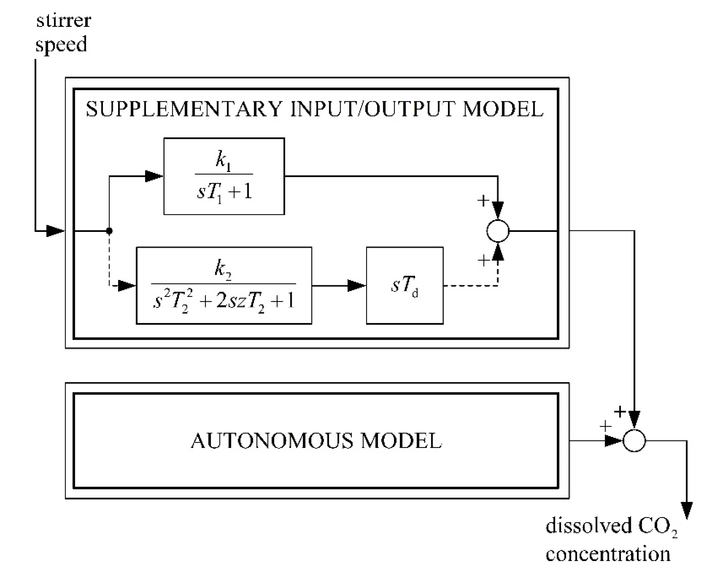
2.1.4. Mathematical Model for a Batch Bioreactor with a Changeable Stirrer Speed

Almost all known mathematical models of batch bioreactors (also this one, presented with Equations (1)–(4)) represent a bioreactor as an autonomous system. They describe only the time responses of the bioreactor’s media concentration on different initial conditions.
These models are not convenient for the design of the bioreactor’s control system, because they do not express the influence of the possible control variables (the stirrer’s drive speed or the heater’s temperature) on the bioreactor’s controlled variables (concentrations of biomass, substrate, and product). Until now, there have only been a few publications available wherein the influence of the heat (temperature) and mechanical work (stirrer’s speed) were studied on the bioprocess’s dynamics.
An original approach based on experimental analysis and theoretical insight used for modelling the bioreactor’s product release has been published in [26,33]. In these papers, the bioreactor’s response to different heater temperatures and stirrer speed variations was investigated in different phases of the fermentation process. The observed bioreactor’s output variable was CO2. The milk fermentation process studied was considered as a two-input (heater’s temperature, stirrer’s speed), one-output (CO2 concentration) dynamic system. The main conclusion of the comprehensive laboratory work was that the batch bioreactor’s mathematical model could be considered as composed of two parts [33]:
  • An autonomous mathematical model, which describes the dynamics of the bioreactor as a response to initial states and assumes constant media temperature and stirrer’s rotation speed.
  • A supplementary input/output mathematical model, which describes the influence of heat or mixing on the CO2 release.
Reference [33] shows that we get a good match between the results of laboratory experiments and simulations if we use the described non-linear fundamental model (1)–(4) for an autonomous model, and we apply a linear input-output model of appropriate level as a supplementary input/output model.
The enhanced mathematical model was developed using a two-stage procedure. Firstly, the determination of the autonomous non-linear third order mathematical model was performed, which describes CO2 release behaviour in response to initial conditions by constant process inputs. Secondly, transfer functions (or Differential Equations) were developed, describing CO2 release according to two changeable process inputs.
For the design and synthesis of the control system, a supplementary input/output mathematical model is crucial. In [33], the order of the supplementary input/output model was obtained by means of systematic research with a least-square identification method for different batch bioreactors and different fermentation media in different phases of fermentation. It was concluded that the heater’s temperature or the stirrer’s speed impact on the CO2 release can be modelled with a dynamical system built of two parallel-connected transfer functions:
  • A first-order term with gain k1 and time constant T1.
  • A second-order term with gain k2, the time constant T2, and damping z, which is in series with a differentiator with the time constant Td.
The first-order term denotes a major (dominant) connection between the bioreactor’s inputs and the dynamics of the CO2 release. The second part (the second order term with the differentiator) has an impact during a transient response, and is important for fine tuning of the controller.
A block diagram of the complete mathematical model of the batch bioreactor is presented in Figure 2.
The parameters of the supplementary mathematical model for a typical batch bioreactor are estimated with data from [26,33] and presented in Table 3.
Figure 3 shows the time responses of the dissolved CO2 concentration (i.e., fermentation product), obtained with the presented enhanced mathematical model. Model parameters for simulations are listed in Table 1 and Table 3. The CO2 responses in the case of constant stirrer speed, and in the case when step change of the stirrer speed at t = 2 h appears, are presented in Figure 3. As expected, the change of the stirrer speed impacted the product concentration increase.
The advantage of this simple enhanced model is that it enables the evaluation of the impact of process input (i.e., stirrer speed) on the course of the fermentation product quantity. The model is presented for its simulation role to test control algorithms and to set up laboratory equipment. Its main assistance is carried out in checking the effectiveness of the control system before the system could be applied to laboratory work with tests, as well as in analysing the impacts and suitability of the parameters of the adaptive mechanism. Therefore, in this paper, the parameters of the laboratory bioreactor model are not identified, but the parameters from the references are used for the calculations [26,33]. Simulation results are not presented nor described in detail, since the emphasis of this article is on the experimental work.
The parameters of the supplementary model change during the operation, i.e., the parameters also change by the transition between different phases of the fermentation process. Because the transition is slow (time constants in minutes or hours), the parameters’ variations are also slow. Due to the constant model structure and the unknown and slowly changeable parameters, the adaptive control represents the relevant control strategy for the batch bioreactor’s control. Obtained simulation results confirmed that the used adaptive control ensured stable operation in all tested models. The parameters of the models suit different real batch bioreactors.

2.2. Control System

2.2.1. Control Theory

The first step in the development of a control theory is to select the control objective. Different control theories express control objectives in different ways. To develop a control system for a batch bioreactor, a special version of MRAC was used, called Adaptive Model-Following Control (AMFC). The proposed AMFC is based on Linear Model-Following Control (LMFC), which uses an explicit model [22]. In the case of LMFC, the control system includes an auxiliary dynamic system called the reference model, which is excited by the same external inputs as the controlled plant. The outputs and/or the state-variables of the reference model represent the necessary control target. AMFC appears like a natural extension of the LMFC with an explicit model when an adaptive design must be considered. To design AMFC systems, an MRAC system was used, with parallel configuration and signal synthesis.
A parallel AMFC system with signal-synthesis adaptation can be outlined briefly with Equations (12)–(18).
The controlled plant is described with the state-space Equation (12):
x ˙ p ( t ) = A p x p ( t ) + B p u p ( t )
where x p ( t ) is the n × 1 controlled plant state-space vector, u p ( t ) is the m × 1 controlled plant input vector, and A p and B p are the controlled plant system and input matrices, respectively, with the appropriate dimensions. The range of plant parameters is assumed to be bounded.
The reference model is described with state-space Equation (13):
x ˙ m ( t ) = A m x m ( t ) + B m u m ( t )
where x m ( t ) is the n × 1 reference model state-space vector, u m ( t ) is the m × 1 reference model input vector, and A m and B m are the reference model system and input matrices, respectively, with the appropriate dimensions. The reference model is assumed to be bounded-input/bounded-state stable.
The error between the reference model state-space vector x m ( t ) and controlled plant state-space vector x p ( t ) is defined as the generalised state error vector, and denoted with e ( t ) :
e ( t ) = x m ( t ) x p ( t )
The control system’s objective is to determine the controlled plant input in such a way that the controlled plant state-space vector will converge to the reference model state-space vector to satisfy Equation (15).
lim t   e ( t ) 0
This aim could be achieved by the generation of the controlled plant input vector u p ( t ) , which will be composed of two components, described in Equation (16)–(18):
u p ( t ) = u p 1 ( t ) + u p 2 ( t )
u p 1 ( t ) = K p x p ( t ) + K m x m ( t ) + K u u m ( t )
u p 2 ( t ) = Δ K p ( e ( t ) , t ) x p ( t ) + Δ K u ( e ( t ) , t ) u m ( t )
where u p 1 ( t ) and u p 2 ( t ) are the m × 1 vector components of the controlled plant input u p ( t ) , K p , K m , and K u are constant matrices of the appropriate dimension, and Δ K p ( e ( t ) , t ) and Δ K u ( e ( t ) , t ) are time-varying matrices of the appropriate dimensions.
The matrices K p , K m , and K u guarantee perfect model-following control to the asymptotically stable reference model with the parameters A m and B m in cases when the controlled plant is linear with known and constant parameters A p and B p by generating the controlled plant input u p ( t ) . This part of the control system is called the Linear Model-Following Controller (LMFC). The solution for K p , K m , and K u , which leads to the perfect model-following control, exists if, and only if, [22]:
rank   B p = rank   [ B p , A m A p ] = rank   [ B p , B m ]
This means that a solution exists if the column vectors of the difference matrix ( A m A p ) and the matrix B m are linearly dependent on the column vectors of the matrix B p . A class of solutions can be obtained using the Penrose pseudo-inverse of B p denoted by B p + . Using B p + , the sufficient conditions for the existence of solutions for the perfect model-following control can be written as:
( I B p B p + ) ( A m A p ) = 0
( I B p B p + ) B m = 0
The conditions (20) and (21) are known as Erzberger’s condition for perfect model-following control [22]. If these conditions are satisfied, then K m K p and K u can be computed directly using Equations (22) and (23):
K m K p = B p + ( A m A p )
K u = B p + B m
The feedback gain matrix K p can be computed independently of the perfect model-following conditions. For example, it can be computed using linear optimal control in order to minimise the effect of state disturbances acting on the plant. However, K p must be such that the resulting K m , which leads to satisfaction of (22), also assures that the matrix ( A m B p K m ) is a Hurwitz matrix [22].
In cases when the controlled plant parameters A p and B p are uncertain and changeable, the u p 1 ( t ) does not assure perfect model-following. The additional controlled plant input u p 2 ( t ) must be generated in this case. The u p 2 ( t ) represents the output of the adaptation mechanism, which will assure that the generalised state error e ( t ) goes to zero under certain conditions.
For the design of the adaptation mechanism and for the proof of the stability of the adaptive control system, the Adaptive Model-Following Control (AMFC) system must be reconfigured into an equivalent feedback system with the linear time-invariant part in the forward path, and with the non-linear time-varying part in the feedback loop [22]. The obtained equivalent feedback system enables the use of Popov’s theory of hyperstability.
The linear time-invariant part in the forward path and the non-linear time-varying part in the feedback loop must be chosen in order to be able to meet the specifications required so that the stability of the adaptive system is assured.
To satisfy the required specifications for the linear time-invariant part in the forward path, the linear compensator described by Equation (24) must be included in the adaptation mechanism:
v ( t ) = D e ( t )
where D denotes the matrix gain of the linear compensator and v ( t ) is the output vector of the linear compensator. The linear compensator’s matrix D must be chosen, in order to assure that the transfer matrix of the equivalent forward block defined by Equation (25) is a strictly positive real transfer matrix:
H ( s ) = D ( s I A m + B p K m ) 1 B p
where H(s) denotes a transfer matrix of the equivalent forward block, I is an identity matrix, and s is a complex variable of the Laplace transform.
For the computation of the linear compensator D, one must solve the Lyapunov Equation (26) after the choice of the weighting matrix Q:
( A m B p K m ) T P + P ( A m B p K m ) = Q
where Q is a chosen positive definite matrix and P is the solution of the Lyapunov equation. Finally, the linear compensator’s matrix D is calculated from P with (27):
D = B p T P
To satisfy the required specifications for the non-linear time-varying part in the feedback loop, the time-varying matrices Δ K p ( e ( t ) , t ) and Δ K u ( e ( t ) , t ) must be calculated by means of Equations (28) and (29):
Δ K p ( e ( t ) , t ) = 0 t F v ( τ ) ( G x p ( τ ) ) T d τ + 0 t F v ( τ ) ( G x p ( τ ) ) T + Δ K p ( 0 )
Δ K u ( e ( t ) , t ) = 0 t M v ( τ ) ( N u m ( τ ) ) T d τ + 0 t M v ( τ ) ( N u m ( τ ) ) T + Δ K u ( 0 )
where matrices F, M, G, and N are positive definite matrices, F and G are positive semi-definite matrices, and Δ K p ( 0 ) and Δ K u ( 0 ) are initial values of the time-varying matrices Δ K p ( e ( t ) , t ) and Δ K u ( e ( t ) , t ) .
A block diagram of the entire adaptive system is presented in Figure 4.

2.2.2. Control System Realisation

The adaptive control system for the batch bioreactor was developed based on the presented AMFC. To obtain high-quality milk products, the quantities of the fermentation process (concentrations of microorganisms, substrate, and product, temperature, etc.) must follow the prescribed reference values. One of the quantities which correlates well with all the important fermentation process quantities is CO2 release. This means that it is possible to assure proper trajectories of the fermentation process quantities by means of the control system, which will assure the proper dynamic profile of the CO2 release. A variable speed stirrer drive was used to assure the prescribed dynamic profile of the CO2 release. The described enhanced mathematical model of the fermentation process in the bioreactor presented was used to determine the order of the reference model and the dimension of the adaptation mechanism. The reference trajectories (reference model) of the bioreactor’s quantities were obtained empirically in such a way that the fermentation would be completed in a shorter time, that the final value of the product would be as high as possible, and that there would be no excessive and sudden changes in the growth of microorganisms during fermentation. The goal of the adaptive control system is to assure the prescribed dynamics of the quantities in the bioreactor in the case of an unknown batch bioreactor, various substrates, microorganisms, and disturbances.
The developed concept presented requires the bioreactor to be equipped with a variable speed stirrer’s drive and a measurement gauge for dissolved CO2 concentration. The mentioned stirrer’s system is capable of altering and maintaining a specified mixing speed in the bioreactor. The majority of contemporary commercial applications of batch bioreactors include the required components, or they are available as accessories. A control module, which would perform the developed control, is conceptualised as an external component (PLC, PC with an added AD/DA periphery, or a dedicated controller). In the case of realisation using the external controller, an application with signal transfer between a controlled plant (i.e., a batch bioreactor with the stirrer’s system and the measurement gauge) and the controller is evidently necessary. An overview of the market was carried out by contacting representatives of producers, such as Metler Toledo. Existing commercial applications of batch bioreactors enable simple analogue signal transfer, with information on dissolved CO2 concentration from the measurement gauge into the external controller (analogue input is necessary). Unfortunately, the existing stirrer’s systems are not customised for setting up a reference value from the external controller. With existing commercial applications of batch bioreactors, a more comprehensive adaptation or upgrade of input-output interfaces is necessary (as was carried out in our case).
A second option is the realisation of a control algorithm within the programme equipment of a batch controller. This option is far less expensive and simpler than the first one, though the second option requires a flexible enough program interface on the batch bioreactor, which would be suitable for the implementation of the adaptive controller.

3. Results and Discussion

A dSpace 1103 controller board was utilised for the prototyping of the proposed adaptive control algorithms. An analogue output module of a basic device, SevenMulti (Metler Toledo), was used for the transfer of the measured signal of the CO2 concentration from the bioreactor system to the control device. The control algorithm (i.e., reference model, control law, and adaptation mechanism) was programmed and uploaded into the controller board. The calculated control signal (i.e., reference speed) was routed to the stirrer drive via the controller’s analogue output. An additional electronic interface was required in the stirrer drive, which allowed the speed reference value to be changed.
The proposed adaptive control was used for the described laboratory batch bioreactor and milk fermentation with kefir grains. The time response of the dissolved CO2 concentration during the fermentation process without a control system is shown in Figure 5. In this case, the stirrer’s speed (n = 80 min−1) stayed constant during the entire fermentation process.
The CO2 time response obtained was similar to the response of the first order differential equations, which is consistent with the known mathematical model of non-controlled fermentation [26]. Deviations from the response of the first order differential equations are a consequence of the nature of the biochemical process itself. Microorganisms’ activity often varies because they are highly sensitive to process condition changes (temperature, concentration, pH), viability changes and mutations. Disturbances are also seen clearly in the time course of the fermentation product. Therefore, the repetition of the fermentation, despite the same initial concentrations and unchanged bioreactor, does not yield exactly the same time responses.
On the basis of systematic tests, it is possible to determine empirically what is the maximum possible achieved product concentration, and what can be the shortest duration of fermentation. Operators of batch bioreactors possess empirical experience on a trajectory of output quantity that ensures a desired yield of a quality product in a fermentation process.
On the basis of systematic tests, it is possible to determine empirically what is the desired final product concentration, and what can be the shortest duration of a fermentation process. Operators of batch bioreactors possess empirical experience on the reference profile of output quantity that ensures high yield of a quality product in a short time.
The presented study does not deal with the methods of determining this optimal reference profile. The primary purpose of this study is the development of a control system that will ensure that the CO2 response will follow the arbitrarily set reference profile.
To estimate the reference CO2 profile for the purposes of our study, we executed the fermentation process with the same mixture systematically, but with different stirrer speeds. Because too high a gradient affects the fermentation process negatively, we tried to estimate the maximum allowable gradient that led to the reference final yield. We chose a similar shape of the reference profile as the CO2 response in the fermentation process, only with a higher maximum gradient and final value. By the measurements of various bioreactors and microorganisms, we found that the CO2 transient in the fermentation process is very similar to the step response of the first order differential equation [26]. Based on the estimated values about maximum allowable gradient 0.57 g/L/h and reference final product concentration 0.8 g/L, we defined the reference profile γr(t) with Equation (30):
γ r ( t ) = 0.8 ( 1 e t 1.4 )
The time course of the reference profile is shown in Figure 6. As can be seen in the Figure 5 and Figure 6, the reference trajectory has a negligible lag phase compared to the non-controlled course, and the acceleration part of the growth phase has a maximum allowed gradient. Therefore, the stationary phase is reached faster, which results in a shortening of the fermentation time. Additionally, the steady state value of the reference trajectory is set higher than the stationary value of the non-controlled fermentation process.
A duty of an adaptive controller is to ensure the time course of the output quantity will follow the prescribed reference trajectory. The time course of the reference trajectory differs from the response of the uncontrolled batch bioreactor. The difference is in the time course of the transitive phenomenon and in the stationary value. From the comparison of the non-controlled and reference CO2 release, we conclude that the task of the adaptive controller will be to increase the gradient of the CO2 release at the beginning of the fermentation process, to achieve higher steady-state value, and to hold the CO2 value in the batch reactor almost constant (the same as prescribed with the reference trajectory) during the last phase of the fermentation process.
A parallel AMFC system was used with signal-synthesis adaptation. Its goal was to achieve that the time response of the CO2 concentration would be as close as possible to the reference profile. It follows that the dynamics of the fermentation process would be similar to the dynamics of the reference model. The selected reference model was determined based on the reference profile defined with Equation (30). The parameters of the reference model were chosen in a way that the step response of the model was equal to the empirically obtained trajectory. The following reference model was obtained:
x ˙ m ( t ) = 0.71   x m ( t ) + 0.57   u m ( t )
The parameters in the adaptation mechanism (i.e., values of D, F, M, G, N, F′, and M′) were estimated with support of a simulation based on a typical enhanced model. The goal was to find such parameters of the adaptation mechanism which ensured stable operation and good dynamic properties in the case of non-linear models of different batch bioreactors. We did not look intentionally for parameters that would ensure optimum operation of the selected batch bioreactor, but we tried to determine as many universal parameters that would ensure good control of various batch bioreactors in the entire range of operation. The selected parameters of the reference model, control law, and adaptation mechanism are presented in Table 4. Since the reference model was of the first degree, all elements are scalar.
The time response of the CO2 release obtained with the AMFC system is shown in Figure 7. The trajectory is almost the same as prescribed with the reference model.
The output of the digital adaptive controller represents the reference signal for the stirrer’s drive system. The reference signal is shown in Figure 8. The oscillations are also a consequence of insufficiently filtered measurement noise.
The actual stirrer’s speed is shown in Figure 9.
From Figure 5, Figure 6 and Figure 7, we can see that the adaptive controller assures that the product quantity of the fermentation process follows the prescribed trajectory of the reference model in spite of the unknown parameters of the controlled plant. From Figure 8 and Figure 9, it is clear that the output signal of the adaptive controller stays in the feasible range. The controller’s output does not exceed the stirrer’s drive maximum or minimum limits (operating range 0–300 min−1).
For comparison, we also carried out the control of the fermentation process of the laboratory batch bioreactor with a conventional linear Proportional-Integral (PI) controller. Since we did not know the mathematical model of the laboratory bioreactor, we used the Ziegler-Nichols step response method for tuning the parameters of the PI-controller. The proportional gain kp = 12 and the time constant Ti = 1.17 of the PI-controller were determined. Figure 10 shows the time course of the dissolved CO2 concentration of the laboratory bioreactor if the conventional PI-controller was used instead of the adaptive controller. Significantly worse tracking of the reference course was the result of a lack of knowledge of the mathematical model of the fermentation process, and, consequently, the approximate synthesis of the regulator parameters. The procedure used to tune the parameters is more intended to eliminate disturbances than track the reference value.

4. Conclusions

The main contribution of this work in bioprocess engineering is the development of a control system that enables control of a time course of a fermentation process in batch bioreactors. In the existing commercial laboratory and industrial batch bioreactors, the fermentation process takes place autonomously. These bioreactors are not equipped with control systems, ensuring an equal fermentation course in different batches and enabling output products of equal quality. Due to the variation of input substances (microorganisms, substrate) and disturbances, fluctuation exists in the quality and quantity of a final product. Two original novelties in the development of the control system are presented, such as:
  • A closed-loop control system was used to control the fermentation process. The control system generates a signal to alter the stirrer speed, based on information on the measured concentration of dissolved CO2.
  • A theory of adaptive model-reference control was used for the design of the control system. The approach enabled self-adjustment of the controller to the controlled batch bioreactor. The presented method requires neither determination of a bioreactor’s mathematical model nor a protracting synthesis of a conventional control system.
Results of our application confirmed that the developed adaptive model-following control ensures close tracking of the bioreactor’s output quantity toward the reference trajectory, including in cases of disturbances.
The benefits of the proposed control against other conventional or advanced control approaches are many: the control maintains the prescribed optimal behaviour of the biochemical process in the case of unknown parameters of the batch bioreactor; the tuning of the controller’s parameters is non-demanding and non-time consuming; the stability of the control system is assured, and simple realisation of the control system is possible. In the fermentation on the laboratory bioreactor used, the fermentation duration was reduced from 10 h to 6 h, and the final concentration of the fermentation product was increased by about 10%.
The successful application of the algorithm proposed in this case study revealed its potential for many biochemical processes of industrial interest. It has shown outstanding results, allowing the system to be operated at a high-performance level in a safe manner. The applicability of the proposed control system is not limited only to the milk fermentation control in batch bioreactors. We are looking forward to upgrading and implementing the obtained academic and laboratory findings with commercial types of bioreactors.
We expect that the development in the field of advanced closed-loop control for fermentation processes will intensify in the near future. It would be reasonable to implement adaptive control methods for similar bioprocesses in batch bioreactors. We estimate that the use of model reference control theory could be very promising.

Author Contributions

Conceptualization, J.R., A.G. and D.P.; Methodology, J.R., A.G. and D.P.; Software, J.R.; Validation, J.R.; Formal Analysis, J.R., A.G. and D.P.; Investigation, J.R., A.G. and D.P.; Data Curation, J.R. and D.P.; Writing – Original Draft Preparation, J.R. and A.G.; Writing – Review & Editing, J.R., A.G. and D.P.; Supervision, J.R. All authors have read and agreed to the published version of the manuscript.

Funding

This research received no external funding.

Institutional Review Board Statement

Not applicable.

Informed Consent Statement

Not applicable.

Data Availability Statement

The data presented in this study are available on request from the corresponding author.

Conflicts of Interest

The authors declare no conflict of interest.

Appendix A

Figure A1 presents the batch bioreactor RC1e from Mettler Toledo that was used for the development and testing of the adaptive control system.
Figure A1. Laboratory batch bioreactor RC1e from Mettler Toledo.
Applsci 10 09118 g0a1

Appendix B

Equations (A1)–(A4) present the system matrix A(t) of the linearised model of the fermentation process of a batch bioreactor:
A ( t ) = [ A 1 ( t ) A 2 ( t ) A 3 ( t ) ]
A 1 ( t ) = [ μ m ( 1 P * ( t ) P m ) S * ( t )   K m + S * ( t )   + ( S * ( t ) ) 2 K i   μ m ( 1 P * ( t ) P m ) S * ( t )   K m + S * ( t )   + ( S * ( t ) ) 2 K i   α μ m ( 1 P * ( t ) P m ) S * ( t )   K m + S * ( t )   + ( S * ( t ) ) 2 K i   + β ]
A 2 ( t ) = [ μ m ( 1 P * ( t ) P m ) X * ( t )   K m + S * ( t ) + ( S * ( t ) ) 2 K i   μ m ( 1 P * ( t ) P m ) S * ( t ) X * ( t ) ( 1 + 2 S * ( t ) K i )   ( K m + S * ( t ) + ( S * ( t ) ) 2 K i   ) 2 μ m ( 1 P * ( t ) P m ) X * ( t )   K m + S * ( t ) + ( S * ( t ) ) 2 K i   + μ m ( 1 P * ( t ) P m ) S * ( t ) X * ( t ) ( 1 + 2 S * ( t ) K i )   ( K m + S * ( t ) + ( S * ( t ) ) 2 K i   ) 2 α ( μ m ( 1 P * ( t ) P m ) X * ( t )   K m + S * ( t ) + ( S * ( t ) ) 2 K i   μ m ( 1 P * ( t ) P m ) S * ( t ) X * ( t ) ( 1 + 2 S * ( t ) K i )   ( K m + S * ( t ) + ( S * ( t ) ) 2 K i   ) 2 ) ]
A 3 ( t ) = [ μ m 1 P m S * ( t ) X * ( t )   K m + S * ( t ) + ( S * ( t ) ) 2 K i   μ m 1 P m S * ( t ) X * ( t )   K m + S * ( t ) + ( S * ( t ) ) 2 K i   α μ m 1 P m S * ( t ) X * ( t )   K m + S * ( t ) + ( S * ( t ) ) 2 K i   ]

References

  1. Doran, P. Bioprocess Engineering Principles, 2nd ed.; Academic Press: London, UK, 2012. [Google Scholar]
  2. Selişteanu, D.; Petre, E.; Şendrescu, D.; Roman, M. Nonlinear indirect adaptive control of a Fed-batch fermentation Bioprocess. In Proceedings of the 17th International Conference on Methods Models in Automation Robotics (MMAR), Miedzyzdroje, Poland, 27–30 August 2012; pp. 367–372. [Google Scholar]
  3. Henson, M.A. Biochemical reactor modeling and control. IEEE Contr. Syst. Mag. 2006, 26, 54–62. [Google Scholar] [CrossRef]
  4. Venkateswarlu, C. Advances in monitoring and state estimation of bioreactors. J. Sci. Ind. Res. 2005, 64, 491–498. [Google Scholar]
  5. Chitra, M.; Pappa, N.; Abraham, A. Dissolved Oxygen Control of Batch Bioreactor using Model Reference Adaptive Control scheme. IFAC-PapersOnLine 2018, 51, 13–18. [Google Scholar] [CrossRef]
  6. Ignatova, M.; Patarinska, T.; Ljubenova, V.; Bůcha, J.; Böhm, J.; Nedoma, P. Adaptive stabilisation of ethanol production during the continuous fermentation of Saccharomyces cerevisiae. IEE Proc. Control Theory Appl. 2003, 150, 666–672. [Google Scholar] [CrossRef]
  7. Peroni, C.V.; Kaisare, N.S.; Lee, J.H. Optimal control of a fed-batch bioreactor using simulation-based approximate dynamic programming. IEEE Trans. Control Syst. Technol. 2005, 13, 786–790. [Google Scholar] [CrossRef]
  8. Åström, K.J.; Kumar, P.R. Automatic Control—A Perspective. In Proceedings of the 36th Chinese Control Conference, Dalian, China, 26–28 July 2017. [Google Scholar]
  9. Abraham, E.; Gupta, S.; Jung, S.; McAfee, E. Bioreactor for Scale-Up: Process Control. In Mesenchymal Stromal Cells; Viswanathan, S., Hematti, P., Eds.; Academic Press: Boston, MA, USA, 2017; pp. 139–178. ISBN 978-0-12-802826-1. [Google Scholar]
  10. Mailleret, L.; Bernard, O.; Steyer, J.-P. Nonlinear adaptive control for bioreactors with unknown kinetics. Automatica 2004, 40, 1379–1385. [Google Scholar] [CrossRef] [Green Version]
  11. Shimizu, K. An overview on the control system design of bioreactors. In Measurement and Control; Springer: Berlin/Heidelberg, Germany, 1993; pp. 65–84, Advances in Biochemical Engineering/Biotechnology; ISBN 978-3-540-47587-3. [Google Scholar]
  12. Petre, E.; Selişteanu, D.; Şendrescu, D. Adaptive and robust-adaptive control strategies for anaerobic wastewater treatment bioprocesses. Chem. Eng. J. 2013, 217, 363–378. [Google Scholar] [CrossRef]
  13. Selişteanu, D.; Petre, E.; Răsvan, V.B. Sliding mode and adaptive sliding-mode control of a class of nonlinear bioprocesses. Int. J. Adapt. Control Signal Process. 2007, 21, 795–822. [Google Scholar] [CrossRef]
  14. Yan, X.; Spurgeon, S.K.; Edwards, C. State and Parameter Estimation for Nonlinear Delay Systems Using Sliding Mode Techniques. IEEE Trans. Autom. Control 2013, 58, 1023–1029. [Google Scholar] [CrossRef]
  15. Estakhrouiyeh, M.R.; Vali, M.; Gharaveisi, A. Application of fractional order iterative learning controller for a type of batch bioreactor. IET Control Theory Appl. 2016, 10, 1374–1383. [Google Scholar] [CrossRef]
  16. Wang, B.; Wang, Z.; Chen, T.; Zhao, X. Development of Novel Bioreactor Control Systems Based on Smart Sensors and Actuators. Front. Bioeng. Biotechnol. 2020, 8. [Google Scholar] [CrossRef] [PubMed]
  17. Narayanan, H.; Luna, M.F.; von Stosch, M.; Bournazou, M.N.C.; Polotti, G.; Morbidelli, M.; Butté, A.; Sokolov, M. Bioprocessing in the Digital Age: The Role of Process Models. Biotechnol. J. 2020, 15, 1900172. [Google Scholar] [CrossRef] [PubMed]
  18. Jewaratnam, J.; Zhang, J.; Hussain, A.; Morris, J. Batch-to-Batch Iterative Learning Control of a Fed-batch Fermentation Process Using Incrementally Updated Models. IFAC Proc. Vol. 2010, 43, 78–83. [Google Scholar] [CrossRef]
  19. Kumar, M.; Prasad, D.; Giri, B.S.; Singh, R.S. Temperature control of fermentation bioreactor for ethanol production using IMC-PID controller. Biotechnol. Rep. 2019, 22, e00319. [Google Scholar] [CrossRef] [PubMed]
  20. De Battista, H.; Jamilis, M.; Garelli, F.; Picó, J. Global stabilisation of continuous bioreactors: Tools for analysis and design of feeding laws. Automatica 2018, 89, 340–348. [Google Scholar] [CrossRef]
  21. Alford, J.S. Bioprocess control: Advances and challenges. Comput. Chem. Eng. 2006, 30, 1464–1475. [Google Scholar] [CrossRef]
  22. Landau, Y.D. Adaptive Control: The Model Reference Approach; Marcel Dekker, Inc.: New York, NY, USA, 1979; ISBN 978-0-8247-6548-4. [Google Scholar]
  23. Wawrzyniak, J.; Kaczyński, Ł.K.; Cais-Sokolińska, D.; Wójtowski, J. Mathematical modelling of ethanol production as a function of temperature during lactic-alcoholic fermentation of goat’s milk after hydrolysis and transgalactosylation of lactose. Measurement 2019, 135, 287–293. [Google Scholar] [CrossRef]
  24. Das, G.; Paramithiotis, S.; Sundaram Sivamaruthi, B.; Wijaya, C.H.; Suharta, S.; Sanlier, N.; Shin, H.-S.; Patra, J.K. Traditional fermented foods with anti-aging effect: A concentric review. Food Res. Int. 2020, 134, 109269. [Google Scholar] [CrossRef]
  25. Ram, Y.; Dellus-Gur, E.; Bibi, M.; Obolski, U.; Berman, J.; Hadany, L. Predicting microbial relative growth in a mixed culture from growth curve data. bioRxiv 2016, 022640. [Google Scholar] [CrossRef] [Green Version]
  26. Goršek, A.; Ritonja, J.; Pečar, D. Mathematical model of CO2 release during milk fermentation using natural kefir grains. J. Sci. Food Agric. 2018, 98, 4680–4684. [Google Scholar] [CrossRef]
  27. Farnworth, E.R. Kefir—A complex probiotic. Food Sci. Technol. Bull. Funct. Foods 2005, 2, 1–17. [Google Scholar] [CrossRef] [Green Version]
  28. Abunde, N.F.; Asiedu, N.Y.; Addo, A. Modeling, simulation and optimal control strategy for batch fermentation processes. Int. J. Ind. Chem. 2019, 10, 67–76. [Google Scholar] [CrossRef] [Green Version]
  29. Caramihai, M.; Severin, I. Bioprocess Modeling and Control. In Biomass Now: Sustainable Growth and Use; BoD—Books on Demand: Norderstedt, Germany, 2013; ISBN 978-953-51-1105-4. [Google Scholar]
  30. Bastin, G.; Dochain, D. On-Line Estimation and Adaptive Control of Bioreactors; Elsevier: Amserdam, The Netherlands, 1990; ISBN 978-0-444-88430-5. [Google Scholar]
  31. Thatipamala, R. On-Line Monitoring, State and Parameter Estimation, Adaptive/Computer Control and Dynamic Optimization of a Continuous Bioreactor. Ph.D. Thesis, University os Saskatchewan, Saskatoon, SK, Canada, 1993. [Google Scholar]
  32. Hjortso, M.A.; Wolenski, P.R. Linear Mathematical Models in Chemical Engineering, 2nd ed.; World Scientific Publishing Company: Singapore, 2018; ISBN 978-981-310-713-7. [Google Scholar]
  33. Ritonja, J.; Gorsek, A.; Pecar, D. Control of Milk Fermentation in Batch Bioreactor. Elektronika ir Elektrotechnika 2020, 26, 4–9. [Google Scholar] [CrossRef] [Green Version]
Figure 1. Time courses of concentrations of microorganisms, substrate, and product of analysed fermentation process in batch bioreactor with constant stirrer speed n = 80 min−1, obtained with a non-linear mathematical model (1)–(4) with the parameters in Table 1.
Applsci 10 09118 g001
Figure 2. Block diagram of the enhanced mathematical model of a fermentation process in a batch bioreactor with changeable stirrer speed.
Applsci 10 09118 g002
Figure 3. Time courses of product concentrations of the analysed fermentation process in a batch bioreactor with constant stirrer speed n = 80 min−1 and in a batch bioreactor with step change of stirrer speed from n = 80 min−1 to n = 110 min−1 at t = 2 h, obtained with the supplemented non-linear/linear mathematical model in Figure 2 with the parameters in Table 1 and Table 3.
Applsci 10 09118 g003
Figure 4. Block diagram of an adaptive model-following control system.
Applsci 10 09118 g004
Figure 5. Time course of dissolved CO2 concentration γ of a non-controlled laboratory batch bioreactor by constant stirrer’s speed n = 80 min−1.
Applsci 10 09118 g005
Figure 6. Time course of dissolved CO2 concentration γ of the chosen reference model for the laboratory batch bioreactor.
Applsci 10 09118 g006
Figure 7. Time course of the dissolved CO2 concentration γ of the laboratory batch bioreactor with an AMFC system; additionally, time courses of the CO2 concentration of the reference model and non-controlled laboratory bioreactor are presented for comparison.
Applsci 10 09118 g007
Figure 8. Time course of the reference signal nr for the stirrer system of the laboratory batch bioreactor with an AMFC system (i.e., output of AMFC controller).
Applsci 10 09118 g008
Figure 9. Time course of the measured stirrer speed n of the laboratory batch bioreactor with an AMFC system.
Applsci 10 09118 g009
Figure 10. Time course of the dissolved CO2 concentration γ of the laboratory batch bioreactor with a PI control system; additionally, the time course of the CO2 concentrations of a non-controlled laboratory bioreactor and the time course of the reference CO2 concentration are presented for comparison.
Applsci 10 09118 g010
Table 1. Parameters and initial values of the non-linear (autonomous) mathematical model of the analysed fermentation process in the batch bioreactor [31].
ParameterValue
The substrate inhibition constant K i = 74.58   g / L
The substrate saturation constant K m = 0.50   g / L
The product inhibition constant P m = 12.60   g / L
The maximum microorganism’s growth rate μ m = 0.45   h 1
The product yield related to microorganism’s growth α = 0.90
The product yield independent of the microorganism’s growth β = 0.001   h 1
The initial value of the concentration of the biomass X ( 0 ) = 2.9   g / L
The initial value of the concentration of the substrate S ( 0 ) = 9.0   g / L
The initial value of the concentration of the product P ( 0 ) = 0.1   g / L
Table 2. Eigenvalues of the linearised mathematical model of a non-linear model of the analysed fermentation process in a batch bioreactor.
t (h)λ1λ2λ3
0.000.000287070.30661
0.500.000386730.27507
1.000.00053650.23768
1.500.000780890.19376
2.000.00124340.14263
2.500.00246560.083038
3.000.0090503 + 0.012248i0.0090503 − 0.012248i
3.50−0.05743−0.0044616
4.00−0.16346−0.0016714
4.50−0.32487−0.00084529
5.00−0.65823−0.00037158
5.50−1.4758−0.00011003
6.00−2.7119−0.000023361
6.50−3.3547−5.869 × 10⁻⁶
7.00−3.5674−1.6476 × 10⁻⁶
7.50−3.6291−4.7436 × 10⁻⁷
8.00−3.6438−1.3728 × 10⁻⁷
8.50−3.6445−3.9785 × 10⁻⁸
9.00−3.6411−1.1467 × 10⁻⁸
9.50−3.6366−3.3178 × 10⁻⁹
10.00−3.6317−9.8953 × 10⁻¹⁰
Table 3. Parameters of the supplementary linear input/output mathematical model, which describes the influence of stirrer speed on the CO2 release of the analysed fermentation process in a batch bioreactor.
k1 = 0.02T1 = 0.5 h
k2 = 0.003T2 = 0.4 hz = 0.26Td = 1.5
Table 4. Parameters of the reference model, control law, and adaptation mechanism for the control of the fermentation process in the laboratory batch bioreactor.
Am = −0.71Bm = 0.57
Kp = 0Km = 0Ku = 0
D = 25G = 10N = 10
F = 10F′ = 10M = 10M′ = 10
Publisher’s Note: MDPI stays neutral with regard to jurisdictional claims in published maps and institutional affiliations.

