Article

Anode Effect Prediction in Hall-Héroult Cells Using Time Series Characteristics

1
Chair of Automation/Computer Science, University of Wuppertal, Rainer-Gruenter-Str. 21, 42119 Wuppertal, Germany
2
TRIMET Aluminium SE, Aluminiumallee 1, 45356 Essen, Germany
*
Author to whom correspondence should be addressed.
Appl. Sci. 2020, 10(24), 9050; https://doi.org/10.3390/app10249050
Submission received: 29 November 2020 / Revised: 11 December 2020 / Accepted: 15 December 2020 / Published: 18 December 2020
(This article belongs to the Special Issue Industry 4.0 Based Smart Manufacturing Systems)

Abstract

:
In aluminium production, anode effects occur when the alumina content in the bath is so low that normal fused salt electrolysis cannot be maintained. This is followed by a rapid increase of pot voltage from about 4.3 V to values in the range from 10 to 80 V. As a result of a local depletion of oxide ions, the cryolite decomposes and forms climate-relevant perfluorocarbon (PFC) gases. The high pot voltage also causes a high energy input, which dissipates as heat. In order to ensure energy-efficient and climate-friendly operation, it is important to predict anode effects in advance so that they can be prevented by prophylactic actions like alumina feeding or beam downward movements. In this paper a classification model is trained with aggregated time series data from TRIMET Aluminium SE Essen (TAE) that is able to predict anode effects at least 1 min in advance. Due to a high imbalance in the class distribution of normal state and labeled anode effect state as well as possible model’s weaknesses the final F1 score of 32.4% is comparatively low. Nevertheless, the prediction provides an indication of possible anode effects and the process control system may react on it. Consequent practical implications will be discussed.

1. Introduction

In the early days of aluminium electrolysis there was no automatic feed control. The operators had to wait until an anode effect (AE) occured, which is always manifested by a rapid increase of pot voltage. Right at the time of occurence they fed the pot with a batch of alumina and waited for the next AE to come. If it came too early the amount of alumina was increased and vice versa. The termination of the AE was established manually with iron rakes or green wood poles. Nowadays there is consens that AEs are detrimental and must be avoided [1,2,3]. Because of the high voltage in the range from 10 to 80 V AEs reduce the energy and current efficiency, induce meltback of the side-ledge and can lead to localized sludging. But furthermore AEs cause emissions of harmful perfluorocarbon (PFC) greenhouse gases, CF4 and C2F6 which have extremely high global warming potentials [2,3,4,5]. Due to the availability of automatic feeders and computer controlled feeding but also automatic AE termination routines the aluminium industry was able to eminently reduce the frequency and duration of AEs [1].
In the last decades there was further improvement and research—Haupin and Seger [1] present different methods for predicting approaching AEs (hysteresis in volt-amp curve, rate of voltage rise, measuring high frequency electrical noise, measuring acoustic noise and pilot anodes) and reduce AE frequency (good condition of pot’s lining and electrical connections, high quality alumina and properly maintained feeders, uniform anode current density and a proper ledge).
Thorhallsson [6] suggests an improved maintenance, more focus on pot tending to reduce AE frequency and a stepwise downward shift of the anode beam with specific delays between separate downward movements and an adjusted feeding strategy during termination to reduce the duration of AEs. Fardeau [7] et al. found that mainly a proper bath height control can reduce AE frequency. Mulder et al. [5] analysed the root causes of AEs and categorised them into three groups: Pot controllers feed strategy, maintenance practices and alumina quality. With the introduction of individual anode current measurement (ACM) new methods and models for predicting AEs were proposed [8,9,10,11]. Since this paper deals with data of pots where no ACM is implemented, thus it is based on classic process data, these papers are not discussed in detail. Regarding prediction models using classic process data, da Costa et al. [12] and Wilson et al. developed [13] univariate threshold-based models. The time difference between the timestamp of detection by the model and the timestamp of detection by the process control system, so called lead time was in the range of seconds. Y. Zhang [14] used wavelet packet transform to analyse the pot resistance for AE prediction. Majid [15] applied multivariate statistical techniques in order to predict AEs. Z. Zhang et al. [16] developed a machine learning model with a lead time of 30 min and an F1 score of 99.8%. Chen et al. [9] used a collaborative two-dimensional forecast model with a lead time of 20 min to 40 min and an accuracy of 95%.
In summary, it can be stated that some predictions methods were only proposed but never applied to a real test dataset of sufficient size or used in a live test scenario. Moreover many authors do not provide enough evaluation criteria like confusion matrix and F1 score. In this paper a classification model based on aggregated time series data is proposed. Preprocessing, training and testing steps including evaluation criteria are presented with high degree of transparency.

2. State of the Art at TAE

The TRIMET Aluminium SE Essen (TAE) plant consists of 360 pots in three production potrooms with EPT-14 PreBaked Point Feeder (PBPF) cells in the first two potrooms and EPT-17 PBPF cells in the third potroom. The prefix EPT stands for “elektronische Prozesssteuerung Tonerde” (computer controlled alumina feed). The number 14 indicates that the potlines originally operated at 140 kA [17]. Under normal process conditions a balanced feed strategy is applied, using a derived pseudo-resistance slope calculation to determine when the feed strategy should change from underfeed to overfeed [5]. During train and test time the first potroom was running at an amperage of 173 kA with a standard deviation of around 5 kA, while the second potroom was running at 165 kA with a standard deviation of around 2.5 kA and the third potroom was running at 171 kA with a standard deviation of only 1 kA.
In industry a commonly used definition for AE detection by the process control system is when pot voltage exceeds 8 V for more than three consecutive seconds [4]. At TAE these thresholds are 7.5 V for 3.96 s. An AE is terminated when pot voltage is below 6.6 V for more than 39.96 consecutive seconds. An example of the voltage behaviour during an AE with four restarts can be seen in Figure 1. The termination of AEs are achieved in a quenching procedure, where the anode beam is lowered and additionally a massive overfeed of alumina is generated.
If this does not attain any success AEs are terminated manually with wood poles. Wong et al. [4] state that beneath conventional AEs (typically start on a few anodes and propagate to all anodes within seconds) there are also so called low voltage propagating AEs (LVP-AE) that exhibit peak voltages that fall below the threshold voltage (<8 V). LVP-AEs have a very similar PFC emission characteristic but their propagation is limited to a section of the pot and after propagation they self terminate. Furthermore Wong et al. found so called non-propagating AEs (NP-AE) with no visible voltage signature. NP-AEs have a different PFC emission characteristic compared to conventional AEs and remain on several localised anodes. It is important to note that Zarouni et al. claim that there is some evidence [18] that LVP-AEs and NP-AEs are more prevalent for large-sized, high amperage (>300 kA) pots. TAE’s pots with a number of 26 anodes and a pot size of 7.2 m × 3.4 m do not belong to the group of large-sized pots.
Currently there is no AE prediction model implemented. As Mulder et al. [5] reported, AEs have only been reduced from a maintenance perspective until now.

3. Anode Effect Prediction

Building a machine learning model consists of different steps that will be presented in the following subsections.

3.1. Data Selection and Preprocessing

Usually in machine learning the whole dataset is splitted into at least training and test data. In this paper the dataset consists of 63% training data (regarding frequency of AEs) and 37% test data both including all 360 pots from all potrooms. It was decided to differ from the well-known 80/20 splitting to have more data for testing, at least half a month. The splitting is shown in the timeline in Figure 2. It is confirmed that in both time intervals the process and the technical state was not altered.
It was decided to use a feature based approach to build the prediction model. Because measured data in aluminium electrolysis process is mainly time series data, it is standing to reason to use time series features. Time series features, also called time series characteristics and especially the usage for classification have gained more attention in the last years. Fulcher et al. [19] analysed over 9000 time series analysis algorithms across an interdisciplinary literature, while Lubba et al. [20] reduced this huge amount to a fixed set of only 22 canonical characteristics, called catch22 used for classification. Hyndman et al. [21] provide a set of 18 features, called tsfeatures. Over the years this set has been continuously extended. In this paper a python implementation of tsfeatures by Garza et al. [22] is used. In general time series characteristics can be seen as a toolbox to solve time series related problems for many domain applications. These characteristics provide a representation of the time series, covering measurements of basic statistics, linear correlations, stationarity, entropy, methods from the physical nonlinear time-series analysis literature, linear and nonlinear model parameters, fits, and predictive power [20]. Lubba et al. [20] show the usability for time series with a fixed length. In contrast in this paper the time series do not have a fixed length because the process is running 24 h per day. For this reason a rolling window approach is used, where the window length and the step size are parameters. This rolling window approach applies to the feature generation using catch22 and tsfeatures but also to other features described in the following paragraphs.
In the first step of feature generation the pot resistance is chosen. Because of the current modulation in potroom 1, the voltage would strongly depend on a change in current, while the resistance is more independent. It is measured in steps of 3 s, or respectively 0.33 Hz measuring frequency. Fulcher et al. [19] state that a time series of less than 1000 samples is short, while Lubba et al. [20] consider a time series of 500 samples to be short. In the AE prediction context on condition of a low measuring frequency it is concluded, that there is a conflict between a sufficient time series length and an observation time that is still in the near of the AE. To cover both, a rolling window with a length of 10 min (200 samples) and a step size of 1 min is used to get information about the short-term behaviour. On this rolling window catch22 and tsfeatures time series characteristics are applied.
Since 200 samples should be considered as a very short time series, not every feature may yield useful results. To get information about the long-term behaviour a second rolling window with a length of 60 min (1200 samples) is used. The step size is limited to 5 min to reduce the calculation time. Some characteristics produced errors during computation, yielded too many special-valued outputs or needed a long calculation time in comparison to others and have therefore been removed. The full list of time series characteristics can be seen in Table 1. Furthermore in a resampling step of 1 min the mean and standard deviation were calculated. After these steps the result is a dataset in steps of 1 min. Using the previously mentioned resistance mean, the percentage change with respect to a rolling median with a length of 60 min was calculated. Additionally the linear trend of the resistance mean with a rolling window of 5 min was calculated.
At TAE more process data (5 min steps) is available that has been included in the dataset: Because of the balanced feed strategy there is a process variable called alumina interval, which gives information in percentage about the current feed phase. Since the minimal feed cycle time is 95 min and the underfeed phases are not fixed, the short-term behaviour is covered with a rolling mean with a length of 60 min and the long-term behaviour is covered with a rolling mean with a length of 8 h. On top of that, the difference between the actual resistance and the lower and upper band was calculated.
A root cause analysis of the train dataset has shown that about 30% of all AEs have a technical cause which is mostly either feeder- or breaker-related. Regarding breaker as a technical cause, this takes up around 9% of all AEs.
This analysis coincides with the findings by Mulder et al. [5] for the same potline but other timespan where breakers as a technical cause were in the range of 9 to 14%. For this reason new features were generated counting error messages by the two breakers each with a rolling window of 60 min and 8 h.
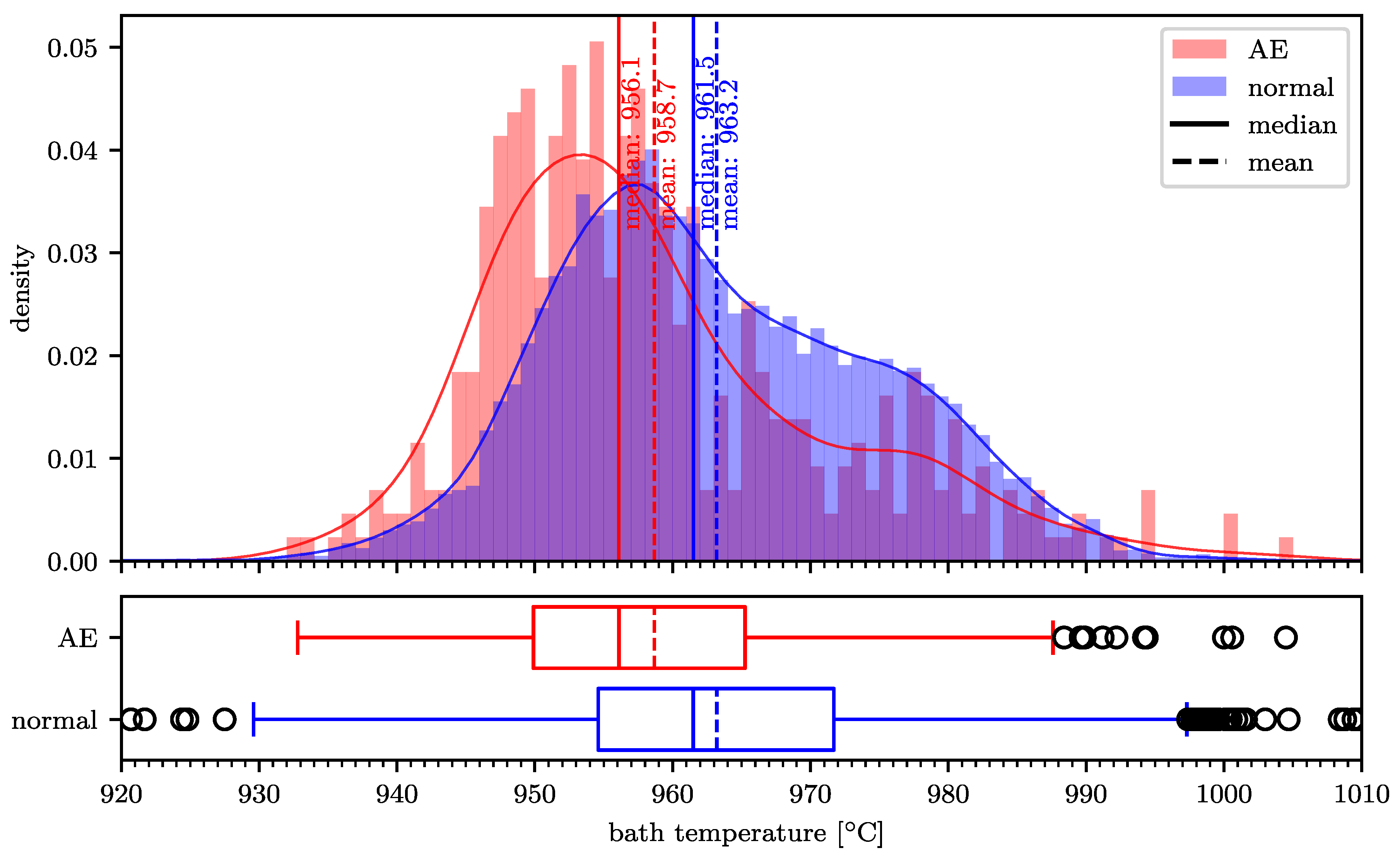
Beside the so called 5 min-data there are manual measurements. Regarding these, only the bath temperature is available on a daily basis. Other measurements are performed less frequently. The univariate distribution of the bath temperature in Figure 3 shows that AEs tend to occur more often at lower bath temperatures. This is because the alumina dissolution is attenuated at lower temperatures [3]. Except for liquidus temperature other manual measurements like for example, bath height, metal height and superheat have distributions of AE and normal state that overlap to a great extent. On this account and the difficulty to impute measurements that are only available every second day or even worse, bath temperature only was merged with the present dataset. An overview of all features that are used as input for the machine learning model can be seen in Figure 4. The bold font denotes list of features. The letter X can be replaced by 1 and 2, because there are two breakers in each pot. All features were merged by time.

3.2. Data Labeling and Dealing with Imbalance

After feature generation and the resultant determination of the smallest time step between two samples, it was possible to label the data. An example of the data labeling is shown in Figure 5. The timestamp of the AE start is available with a resolution of seconds. All samples where the timedelta until AE start is less than 1 min is labeled as 0. All samples where the timedelta until AE start is at least 1 min up to 2 min is labeled as 1. This procedure continues until the label 10 is generated. The timestamp of AE termination is also available with a resolution of seconds and is rounded up to the next full minute. All samples that are between the AE start and the modified AE end get the label AE. Finally all other samples are labeled as normal. To create the final dataset only samples with the label 1 (minority class) and normal (majority class) are kept. This ensures that the lead time is at least 1 min.
Regarding samples with the label 1 a prevalence of 0.0035% for train dataset (0.0034% test dataset) was calculated. This means that there is a severe imbalance between normal state and AE state. Another common term to describe an imbalance is the imbalance ratio (IR). It is defined as the number of negative class samples divided by the number of positive class samples [23]. For the train and test dataset IR is about 29,000. Fernandez et al. [23] state that the most well-known repository for imbalanced datasets is the knowledge extraction based on evolutionary learning (KEEL) repository. Looking at the IR value from these datasets one can observe that it is not typically larger than 100. Krawczyk [24] criticises that there is a lack of studies on the classification of extremely imbalanced datasets. He states in real-life applications such as fraud detection or cheminformatics the imbalance ratio would be ranging from 1000 to 5000. According to that, it is important to note that the dataset in this paper belongs to the group of extremely imbalanced datasets. In literature there are three main techniques to deal with imbalance in classification. First it is possible to upsample the minority class, second downsample the majority class or third using cost-sensitive machine learning algorithms [25]. In this paper a combination of the last two techniques is used. In the first step the majority class is downsampled. For this purpose the imbalanced-learn package (version 0.7.0) by Lemaitre et al. [26] is used. The aim is to resize the training dataset, which contains over 12 million samples, so that the following training step does not take time in the order of days. In contrast to cleaning undersampling techniques, controlled undersampling techniques allow to specify the class ratios. In this paper RandomUndersampler and NearMiss are used. While RandomUndersampler randomly selects a subset of data, NearMiss implements three different types of heuristic—NearMiss-1 selects majority class examples with minimum average distance to n closest minority class examples. NearMiss-2 selects majority class examples with minimum average distance to n furthest minority class examples. At the last NearMiss-3 selects majority class examples with minimum distance to each minority class example [25,26].

3.3. Machine Learning Model

After undersampling the reduced training dataset is used as input for a machine learning model. Because the reduced training dataset is still imbalanced, cost-sensitive machine learning algorithms are applied. Scikit-learn (version 0.23.2) [27] implementations of Logistic Regression, Random Forest Classifier and Linear Support Vector Classifier support class weights, which penalize the models more for errors made on samples from the minority class and are therefore used. Furthermore an implementation of gradient boosting, eXtreme Gradient Boosting (version 0.90) by Chen and Guestrin [28] is used, which also supports class weights. All models are classifiers with a binary output. The simplest models are Logistic Regression and Linear Support Vector Classifier, which are only able to create a linear decision boundary. In general linear models are good for large datasets and very high dimensional data. In particular Support Vector Classifiers are sensitive to hyperparameters. Random Forests are robust and more powerful than linear models but may suffer from high dimensional sparse data. Gradient boosting machines may be slightly more powerful than Random Forests, but need more hyperparameter tuning than Random Forests [29]. For models that are not tree-based and not able to do a feature selection (Logistic Regression and Support Vector Classifier) a recursive feature elimination is performed beforehand. In addition the models are also trained without any recursive feature elimination. To find appropriate hyperparameters a gridsearch is done. The hyperparameter space is shown in Table 2. As validation strategies a KFold and Stratified KFold with 10 splits are chosen. The scoring is evaluated with the help of the F1 score.

4. Results

The training was performed with different feature combinations as input. Moreover the hyperparameters of the undersampling techniques were varied, resulting in different IR values.
These combinations are shown in Table 3. In general it can be observed that the Random Forest Classifier always turns out to be the best model. If no time series features are used (#1) the score is low. The same applies if the RandomUndersampler (#2, #12) or NearMiss-1 (#3, #13) is used. NearMiss-2 could not be tested due to excessive memory consumption. The best results are obtained by the use of time series features and NearMiss-3 with an IR of 9 (#6, #16). The confusion matrices of these two best models regarding F1 score can be seen in Figure 6.

5. Post Analysis and Discussion

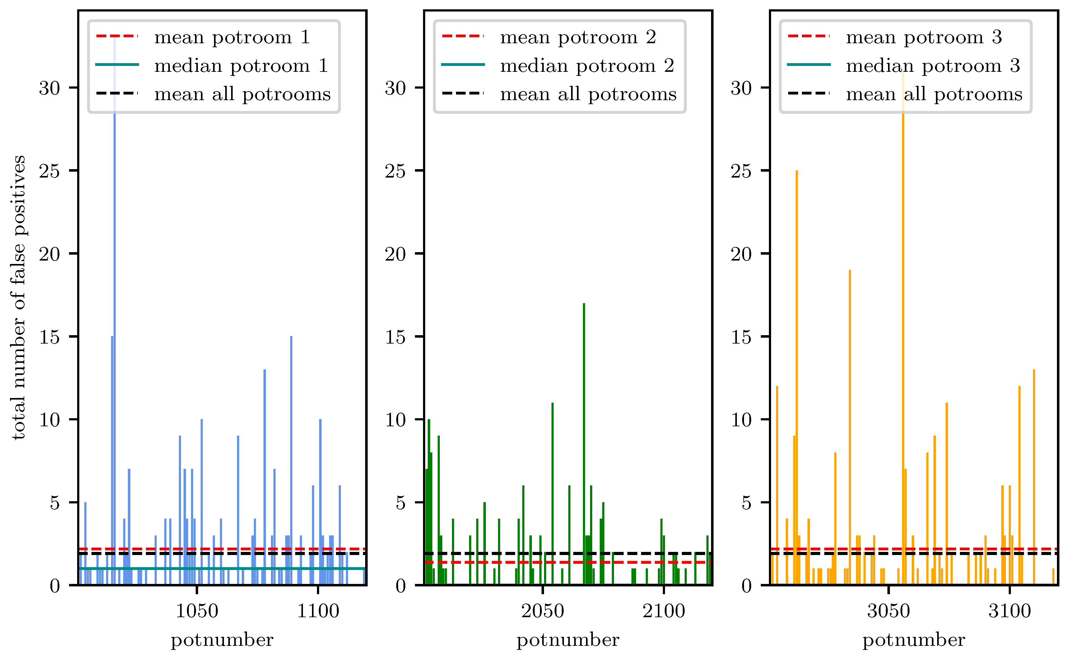
Because the number of false positives is higher than the true positives it was decided to do a post analysis. For the analysis the best model was chosen (#16, see Table 3). First of all the distribution of false positives dependent on the potnumber is investigated, shown in Figure 7. It can be observed that the false positives are not uniformly distributed. Some potnumbers exhibit considerably more false positives than others. One reason for this is the accumulation of false positives in groups of consecutive time steps. Among the potrooms the differences are small. A further analysis on a sample basis regarding the prediction over time shows that some false positives are related to events like anode change, metal tapping and current drop. Disabling the model for 3 h after restart in consequence of a current drop and for 30 min after anode change can improve the score slightly. Disabling the model during other events does not increase the scoring. Removing false positives if the prediction is up to 30 min in advance also yields an improvement.
Finally the number of false positives decreases to 570 while the true positives reduce to 163 and therefore the F1 score increases to 32.4%. Regarding the false positives again, the previously mentioned LVP-AEs need also to be taken into account. It was observed that some false positives occur in the presence of a rapid increase of voltage which did not cross the threshold voltage of 7.5 V.
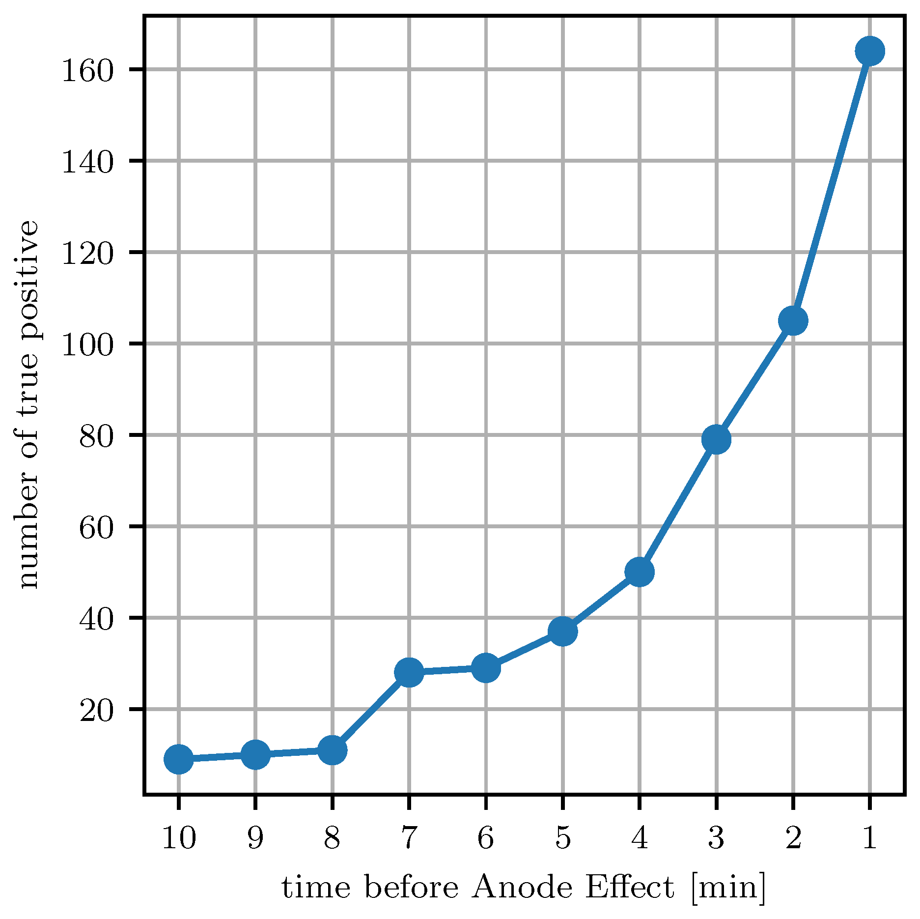
Since the data was labeled up to 10 min in advance before AE, it was possible to apply the model to these samples and analyse the lead time, see Figure 8. About 50% of all true positives are predicted 3 min in advance, while 35% of all true positives have a lead time of 1 min.

6. Conclusions

In this paper a classification model was trained that is able to predict AEs at least 1 min in advance. It was shown that time series features/characteristics can improve the model’s performance significantly. Since AEs occur rarely and a time base of 1 min was chosen, the dataset was extremely imbalanced. A combination of undersampling and cost-sensitive algorithms was proposed to solve this problem. The F1 score of the best model, namely a Random Forest Classifier is about 29.3%. A post analysis showed that disabling removing false positives if the prediction is up to 30 min in advance and disabling the model during events can increase the F1 score to 32.4%. Nevertheless in comparison to Reference [16] the F1 is low and needs to be improved. Including a low frequency and high frequency filtered noise signal, which will be available in future may improve the score. In future also live tests should be performed to prove if the lead time is sufficient and in general which actions like alumina feeding or beam downward movements are promising to prevent anode effects. In addition it needs to be examined if the amount of false positive are detrimental for the pot’s condition. For example a pot might be in an underfeed phase, right before turning into overfeed phase. An additional feeding to prevent the anode effect might not create any disadvantages, for example, due to sludge accumulation. But still there are open questions. Like Mulder et al. [5] said “a cell having AEs is synonymous to having a problem”, this would mean that preventing AEs only does not fix the root cause. However the symptoms of harmful PFC gases and reduced energy and current efficiency may be avoided for the most part.

Author Contributions

Conceptualization, R.K. and N.G.; methodology, R.K.; software, R.K.; validation, R.K.; formal analysis, R.K.; investigation, R.K. and A.M.; resources, R.K. and A.M.; data curation, R.K.; writing—original draft preparation, R.K.; writing—review and editing, R.K., N.G., R.D., A.M. and D.T.; visualization, R.K.; supervision, D.T.; project administration, D.T.; funding acquisition, R.K., N.G. and D.T. All authors have read and agreed to the published version of the manuscript.

Funding

This research was funded by Bundesministerium für Bildung und Forschung (03SFK3B1-2).

Acknowledgments

Authors would like to thank their industrial partner, TRIMET Aluminium SE for collaboration on this project.

Conflicts of Interest

The authors declare no conflict of interest.

Abbreviations

The following abbreviations are used in this manuscript:
TAETRIMET Aluminium SE Essen
AEanode effect
PFCperfluorocarbon
ACManode current measurement
LVP-AElow voltage propagating anode effects
NP-AEnon-propagating anode effects
IRimbalance ratio
KEELknowledge extraction based on evolutionary learning

References

  1. Haupin, W.; Seger, E.J. Aiming for Zero Anode Effects. In Essential Readings in Light Metals: Volume 2 Aluminum Reduction Technology; Springer International Publishing: Berlin/Heidelberg, Germany, 2016; pp. 767–773. [Google Scholar] [CrossRef]
  2. Grjotheim, K.; Kvande, H. Introduction to Aluminium Electrolysis; Alu Media GmbH: Düsseldorf, Germany, 1993. [Google Scholar]
  3. Thonstad, J.; Utigard, T.A.; Vogt, H. On the anode effect in aluminum electrolysis. In Essential Readings in Light Metals: Volume 2 Aluminum Reduction Technology; Springer International Publishing: Berlin/Heidelberg, Germany, 2016; pp. 131–138. [Google Scholar] [CrossRef]
  4. Wong, D.S.; Tabereaux, A.; Lavoie, P. Anode Effect Phenomena During Conventional AEs, Low Voltage Propagating AEs & Non-Propagating AEs. In Light Metals 2014; Springer: Cham, Switzerland, 2014; pp. 529–534. [Google Scholar] [CrossRef]
  5. Mulder, A.; Lavoie, P.; Düssel, R. Effect of Early Abnormality Detection and Feed Control Improvement on Reduction Cells Performance. In Proceedings of the 12th Australasian Aluminium Smelting Technology Conference, Queenstown, New Zealand, 2–7 December 2018. [Google Scholar]
  6. Thorhallsson, A.I. Anode Effect Reduction at Nordural—Practical Points. In Light Metals 2015; Springer: Cham, Switzerland, 2015; pp. 539–542. [Google Scholar] [CrossRef]
  7. Fardeau, S.; Martel, A.; Marcellin, P.; Richard, P. Statistical Evaluation and Modeling of the Link between Anode Effects and Bath Height, and Implications for the ALPSYS Pot Control System. In Light Metals 2014; Springer: Cham, Switzerland, 2014; pp. 845–850. [Google Scholar] [CrossRef]
  8. Kremser, R.; Grabowski, N.; Düssel, R.; Kessel, K.; Tutsch, D. Investigation of Different Measurement Techniques for Individual Anode Currents in Hall-Héroult Cells. In Proceedings of the 12th Australasian Aluminium Smelting Technology Conference, Queenstown, New Zealand, 2–7 December 2018. [Google Scholar]
  9. Chen, Z.; Li, Y.; Chen, X.; Yang, C.; Gui, W. Anode effect prediction based on collaborative two-dimensional forecast model in aluminum electrolysis production. J. Ind. Manag. Optim. 2019, 15, 595–618. [Google Scholar] [CrossRef] [Green Version]
  10. Dion, L.; Lagacé, C.; Laflamme, F.; Godefroy, A.; Evans, J.W.; Kiss, L.I.; Poncsák, S. Preventive Treatment of Anode Effects Using on-Line Individual Anode Current Monitoring. In Light Metals 2017; Springer: Cham, Switzerland, 2017; pp. 509–517. [Google Scholar] [CrossRef]
  11. Cheung, C.; Menictas, C.; Bao, J.; Skyllas-Kazacos, M.; Welch, B.J. Frequency response analysis of anode current signals as a diagnostic aid for detecting approaching anode effects in aluminum smelting cells. In Light Metals 2013; Springer International Publishing: Cham, Switzerland, 2003; pp. 887–892. [Google Scholar] [CrossRef]
  12. da Costa, F.; Paulino, L. Computer Algorithm to predict Anode effect Events. In Light Metals 2012; Springer: Cham, Switzerland, 2012; pp. 655–656. [Google Scholar] [CrossRef]
  13. Wilson, A.; Illingworth, M.; Pearman, M. Anode Effect Prediction and Pre-Emptive Treatment at Pacific Aluminium. In Proceedings of the 12th Australasian Aluminium Smelting Technology Conference, Queenstown, New Zealand, 2–7 December 2018. [Google Scholar]
  14. Zhang, Y. Study on Anode Effect Prediction of Aluminium Reduction Applying Wavelet Packet Transform. In Communications in Computer and Information Science; Springer Berlin Heidelberg: Berlin/Heidelberg, Germany, 2010; pp. 477–484. [Google Scholar] [CrossRef]
  15. Majid, N. Cascade Fault Detection and Diagnosis for the Aluminium Smelting Process using Multivariate Statistical Techniques. Ph.D. Thesis, The University of Auckland, Auckland, New Zealand, 2011. [Google Scholar]
  16. Zhang, Z.; Xu, G.; Wang, H.; Zhou, K. Anode Effect prediction based on Expectation Maximization and XGBoost model. In Proceedings of the 2018 IEEE 7th Data Driven Control and Learning Systems Conference, Enshi, China, 25–27 May 2018; pp. 560–564. [Google Scholar] [CrossRef]
  17. Tabereaux, A. Prebake cell technology: A global review. JOM 2000, 52, 23–29. [Google Scholar] [CrossRef]
  18. Zarouni, A.; Reverdy, M.; Zarouni, A.A.; Venkatasubramaniam, K.G. A Study of Low Voltage PFC Emissions at Dubal. In Light Metals 2013; Springer International Publishing: Cham, Switzerland, 2013; pp. 859–863. [Google Scholar] [CrossRef]
  19. Fulcher, B.D.; Little, M.A.; Jones, N.S. Highly comparative time-series analysis: The empirical structure of time series and their methods. J. R. Soc. Interface 2013, 10, 20130048. [Google Scholar] [CrossRef] [PubMed]
  20. Lubba, C.H.; Sethi, S.S.; Knaute, P.; Schultz, S.R.; Fulcher, B.D.; Jones, N.S. catch22: CAnonical Time-series CHaracteristics. Data Min. Knowl. Discov. 2019, 33, 1821–1852. [Google Scholar] [CrossRef] [Green Version]
  21. Hyndman, R.; Wang, E.; Laptev, N. Large-Scale Unusual Time Series Detection. In Proceedings of the 2015 IEEE International Conference on Data Mining Workshop (ICDMW), Atlantic City, NJ, USA, 14–17 November 2015. [Google Scholar] [CrossRef]
  22. Garza, F.; Gutierrez, K.; Challu, C.; Moralez, J.; Olivares, R.; Mergenthaler, M. tsfeatures. Available online: https://github.com/FedericoGarza/tsfeatures (accessed on 10 November 2020).
  23. Fernández, A.; García, S.; Galar, M.; Prati, R.C.; Krawczyk, B.; Herrera, F. Learning from Imbalanced Data Sets; Springer International Publishing: Berlin/Heidelberg, Germany, 2018. [Google Scholar]
  24. Krawczyk, B. Learning from imbalanced data: Open challenges and future directions. Prog. Artif. Intell. 2016, 5, 221–232. [Google Scholar] [CrossRef] [Green Version]
  25. Brownlee, J. Imbalanced Classification with Python: Better Metrics, Balance Skewed Classes, Cost-Sensitive Learning; Machine Learning Mastery: Vermont Victoria, Australia, 2020. [Google Scholar]
  26. Lemaître, G.; Nogueira, F.; Aridas, C.K. Imbalanced-learn: A Python Toolbox to Tackle the Curse of Imbalanced Datasets in Machine Learning. J. Mach. Learn. Res. 2017, 18, 559–563. [Google Scholar]
  27. Pedregosa, F.; Varoquaux, G.; Gramfort, A.; Michel, V.; Thirion, B.; Grisel, O.; Blondel, M.; Prettenhofer, P.; Weiss, R.; Dubourg, V.; et al. Scikit-learn: Machine Learning in Python. J. Mach. Learn. Res. 2011, 12, 2825–2830. [Google Scholar]
  28. Chen, T.; Guestrin, C. XGBoost: A Scalable Tree Boosting System. In Proceedings of the 22nd ACM SIGKDD International Conference on Knowledge Discovery and Data Mining, KDD ’16, San Francisco, CA, USA, 13–17 August 2016; pp. 785–794. [Google Scholar] [CrossRef] [Green Version]
  29. Müller, A.C.; Guido, S. Introduction to Machine Learning with Python: A Guide for Data Scientists; O’Reilly Media: Sebastopol, CA, USA, 2016. [Google Scholar]
Figure 1. Example of voltage behaviour during an anode effect (AE) with four restarts from train dataset.
Applsci 10 09050 g001
Figure 2. Splitting of train and test dataset.
Applsci 10 09050 g002
Figure 3. Distribution of bath temperature in training dataset.
Applsci 10 09050 g003
Figure 4. Features used as input for machine learning model.
Applsci 10 09050 g004
Figure 5. Example of data labeling.
Applsci 10 09050 g005
Figure 6. Confusion matrices of the two best models (#6, #16), see Table 3.
Applsci 10 09050 g006
Figure 7. Distribution of false positives dependent on potnumber.
Applsci 10 09050 g007
Figure 8. Lead time of prediction.
Applsci 10 09050 g008
Table 1. Time series characteristics used for feature generation with a rolling window.
TsfeaturesCatch22
acf_features_x_acf1DN_HistogramMode_5
acf_features_x_acf10DN_HistogramMode_10
acf_features_diff1_acf1CO_f1ecac
acf_features_diff1_acf10CO_FirstMin_ac
acf_features_diff2_acf1CO_HistogramAMI_even_2_5
acf_features_diff2_acf10CO_trev_1_num
count_entropyMD_hrv_classic_pnn40
crossing_pointsSB_BinaryStats_mean_longstretch1
flat_spotsSB_TransitionMatrix_3ac_sumdiagcov
lumpinessPD_PeriodicityWang_th0_01
nonlinearityIN_AutoMutualInfoStats_40_gaussian_fmmi
sparsityFC_LocalSimple_mean1_tauresrat
stabilityDN_OutlierInclude_p_001_mdrmd
unitroot_kpssDN_OutlierInclude_n_001_mdrmd
unitroot_ppSP_Summaries_welch_rect_area_5_1
SB_BinaryStats_diff_longstretch0
SB_MotifThree_quantile_hh
SC_FluctAnal_2_rsrangefit_50_1_logi_prop_r1
SC_FluctAnal_2_dfa_50_1_2_logi_prop_r1
SP_Summaries_welch_rect_centroid
FC_LocalSimple_mean3_stderr
Table 2. Gridsearch hyperparameter space.
Logistic Regressionpenalty: [ l 1 , l 2 ]
C: [ 0.001 , 0.01 , 0.1 , 1 , 10 , 100 , 1000 ]
Random Forest Classifiern_estimators: [ 1000 ]
max_features: [ 0.3 , 0.5 , 0.7 ]
max_depth: [ 10 , 20 , 30 ]
min_samples_split: [ 2 , 3 ]
min_samples_leaf: [ 1 , 2 ]
eXtreme Gradient Boostingn_estimators: [ 10 , 100 , 500 , 1000 ]
learning_rate: [ 0.001 , 0.01 , 0.1 , 0.3 ]
max_depth: [ 4 , 6 , 8 , 10 ]
Linear Support Vector Classifierpenalty: [ l 1 , l 2 ]
C: [ 0.001 , 0.1 , 1 , 5 , 10 , 50 , 100 ]
Table 3. Results on test dataset
#FeaturesSamplingBest ValidationBest ModelF1 [ % ]
1all features except all time series featuresNearMiss-3
IR = 7
KFoldRandom
Forest
0.8
2all features except catch22 ( 60 min , 5 min )
and tsfeatures ( 60 min , 5 min )
Random
Undersampler
IR = 7
KFoldRandom
Forest
0.5
3all features except catch22 ( 60 min , 5 min )
and tsfeatures ( 60 min , 5 min )
NearMiss-1
IR = 7
allall0
4all features except catch22 ( 60 min , 5 min )
and tsfeatures ( 60 min , 5 min )
NearMiss-3
IR = 7
Stratified KFoldRandom
Forest
15.7
5all features except catch22 ( 60 min , 5 min )
and tsfeatures ( 60 min , 5 min )
NearMiss-3
IR = 8
Stratified KFoldRandom
Forest
16.8
6all features except catch22 ( 60 min , 5 min )
and tsfeatures ( 60 min , 5 min )
NearMiss-3
IR = 9
KFoldRandom
Forest
27.4
7all features except catch22 ( 60 min , 5 min )
and tsfeatures ( 60 min , 5 min )
NearMiss-3
IR = 10
KFoldRandom
Forest
17.8
8all features except catch22 ( 60 min , 5 min )
and tsfeatures ( 60 min , 5 min )
NearMiss-3
IR = 11
KFoldRandom
Forest
18.6
9all features except catch22 ( 60 min , 5 min )
and tsfeatures ( 60 min , 5 min )
NearMiss-3
IR = 12
KFoldRandom
Forest
18.7
10all features except catch22 ( 60 min , 5 min )
and tsfeatures ( 60 min , 5 min )
NearMiss-3
IR = 13
KFoldRandom
Forest
18.9
11all features except catch22 ( 10 min , 1 min )
and tsfeatures ( 10 min , 1 min )
NearMiss-3
IR = 7
Stratified KFoldRandom
Forest
3.9
12all featuresRandom
Undersampler
IR = 7
Stratified KFoldRandom
Forest
0.7
13all featuresNearMiss-1
IR = 7
allall0
14all featuresNearMiss-3
IR = 7
KFoldRandom
Forest
15.2
15all featuresNearMiss-3
IR = 8
Stratified KFoldRandom
Forest
14.4
16all featuresNearMiss-3
IR = 9
KFoldRandom
Forest
29.3
17all featuresNearMiss-3
IR = 10
KFoldRandom
Forest
15.7
18all featuresNearMiss-3
IR = 11
KFoldRandom
Forest
15.4
19all featuresNearMiss-3
IR = 12
KFoldRandom
Forest
15.8
20all featuresNearMiss-3
IR = 13
KFoldRandom
Forest
15.3
Publisher’s Note: MDPI stays neutral with regard to jurisdictional claims in published maps and institutional affiliations.