Abstract
One challenging aspect of therapy optimization and application of control algorithms in the field of tumor growth modeling is the limited number of measurable physiological signals—state variables—and the knowledge of model parameters. A possible solution to provide such information is the application of observer or state estimator. One of the most widely applied estimators for nonlinear problems is the extended Kalman filter (EKF). In this study, a moving horizon estimation (MHE)-based observer is developed and compared to an optimized EKF. The observers utilize a third-order tumor growth model. The performance of the observers is tested on measurements gathered from a laboratory mice trial using chemotherapeutic drug. The proposed MHE is designed to be suitable for closed-loop applications and yields simultaneous state and parameter estimation.
1. Introduction
Cancer treatment and its related fields are intensively studied subjects, since cancer is a major cause of death globally. It is estimated that there will be 21.4 million cases annually by 2030 [1,2]. The application of modern control algorithms for cancer treatment has much potential—especially in the adjustment of the dosages—however, there are difficulties as well [3]. The article investigates a facet of a larger project. The larger project aims to minimize the amount of administered chemotherapeutic drug—while retaining its effect—by applying personalized treatments. Lower amount of doses expected to reduce side effects and potentially postpone the emergence of tumor resistance. One approach is the utilization of feedback control, where the controller (which decides about the drug administration scheme) adapts to the patient. Based on mathematical models accurately describing the underlying physiological processes the professionals have the possibility to define appropriate therapies. System engineers thrive to provide a proper description of the tumor growth, however, the inter- and intrapatient variability and the effects of different drugs are cumbersome to model. Several models were introduced over the years [4,5,6,7,8,9]. In particular, we are concerned with the use of a third-order model. The model describes the dynamics of the living and dead tumor cells, as well as drug concentration [7]. The output of the system is the total tumor volume (sum of the living and the dead tumor volumes).
In tumor growth modeling there are variables that cannot be measured, or are not feasible to measure in practice on a day-to-day basis. Such variables in this particular case are the individual volume of the living and dead tumor cells and drug concentration or the model parameters characterizing the patient variability. A mathematical model gives the general behavior of the system. The general structure can be tailored to each individual by the model parameters. For instance, there is a parameter that corresponds to the clearence of the drug, which can vary from patient to patient. Although they cannot be measured, they play an important role in describing the dynamics of the system and are often required for specific therapy optimization or closed-loop algorithms. In order to extract those unmeasurable variables, usually, an observer is applied. The goal of an observer is to provide information about the inner state variables or parameters based on the measurements. The most common algorithm is the Kalman filter (KF) [10], however, other approaches like sliding mode observer, particle filter [11], linear observer [12] or moving horizon estimation (MHE) [13] are also employed. The latter one is an optimization-based approach, where the name suggests that the optimization is performed on a moving window. The window makes it possible to take into account a series of measurements, and the optimization makes it possible to define application-specific constraints and penalizations. In this paper, an MHE is developed and its performance is compared to an optimized extended Kalman filter (EKF). Often, the drawback of the studies, e.g., [10,11,12,13] is that they are performed on simulated data which is favorable from several aspects. In contrast, this study is evaluated on laboratory measurements, where noise, irregular sampling times and most importantly, structural mismatch are present.
The paper is structured as follows. Section 2.2 describes the utilized third-order tumor growth model and previously identified parameter sets. In Section 2.3 and Section 2.4 first theoretical, general description for the EKF and MHE based observers are given. Thereafter the observers are applied to the specific tumor growth model. Measurement noise is characterized in Section 2.3.1. Sections describing the observers end with the tuning methods. In Section 3 the results are summarized. The observers are evaluated based on their capabilities following the trends of the measurements. During the assessment, the fluctuations of the parameters are taken into account too. Furthermore, different window lengths of the MHE are investigated as well. Finally, in Section 4 and Section 5 the paper is concluded.
2. Materials and Methods
2.1. Experimental Data
The experiments were conducted by the Membrane Protein Research Group of the Research Centre for Natural Sciences published in [14]. The mice are identified with the “PLD” acronym, indicating that the injected chemotherapeutic drug was the pegylated liposomal doxorubicin (PLD) during the experiments. In this trial tumor pieces from a Brca1-/-;p53-/- mouse tumor were transplanted orthotopically to syngenic FVB mice to reduce the time of tumor formation. The tumor volume was measured by calipers every 1–5 days. The treatment protocol was a dynamic reactive approach which was defined as follows. The mice were treated based on the decision of the professionals. The injection could be granted if the tumor volume reached 200 [mm] and at least 10 days past since the last treatment. The injected drug was the maximum tolerable dose 8 [mg/kg] every time. The experiment focused on the elimination of the primary tumor. The experiment was stopped when the tumor volume grew above the 2000 [mm] threshold.
In Figure 1, an example is given of the trial. The raw caliper measurements are represented with black circles, the treatment threshold is plotted with a dashed grey line and the solid green line is a linear interpolation between the measurements. It can be seen that the particular mouse responded well to the treatment, since the volume decreased after the injections. However, some mice develop resistance and the drug stops taking effect (meaning continuously growing volume regardless of the presence of the drug). Those who developed resistance are not taken into account in this study as the applied model does not consider resistance. As a result, data from mice PLD1, PLD2 and PLD8 from [14] are not used in this study.
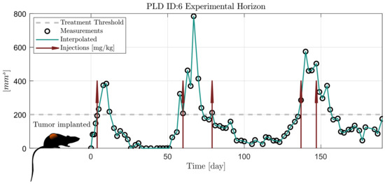
Figure 1.
Scheme of the experiment from [14].
2.2. The Applied Tumor Growth Model
The investigated tumor growth model is a third-order nonlinear ordinary differential equation. The model differentiates between living and dead tumor cell volumes by introducing separate state variables: [mm3] and [mm3], respectively. The third variable [mg/kg] describes the drug concentration in the host. The dynamics is described by the equations given in [6,7] at time t as
where a describes the proliferation rate of the living tumor cells, n is the tumor cell necrosis rate, w is the dead tumor cell washout rate, c is the drug depletion rate. The pharmacodynamics is affected by the b and (median effective dose) parameters. The effect of the drug and the depletion of the drug is characeterized by equations following the dynamics of Michaelis–Menten kinetics, thus and are Michelis–Menten parameters. Resistance is not modeled explicitly, but the ineffectiveness of the drug appears as a specific combination of the parameters. When the difference , the drug is not able to shrink the volume, it only decreases the growth rate. Qualitative analysis of the model has been previously done in [15]. The values of the parameters for the mice identified based on a mixed-effect model [7] are given in Table 1.

Table 1.
The identified parameters of the mice from experiment specified in [14] using a mixed-effect model [7], along with the mean values and standart deiations for each parameter.
2.3. Extended Kalman Filter
For nonlinear systems one of the most widely applied observer is the EKF. First, assume a general system given in the form of:
where f describes the nonlinear system dynamics, h is the output equation, is the additive process noise or disturbance and is the measurement noise. Equation (4) is generalized further with the augmentation of system parameters , where is the original state vector and is the parameter vector.
Since the measurements are done only at discrete times, continuous-discrete EKF has been applied. In the prediction step the model and covariances are propagated using the forward Euler method with shorter sampling times. The equations of the prediction step in time instant t are defined as
where is the error covariance matrix, is the Jacobian matrix of the system and is the process noise covariance matrix. The update step in the k-th discrete step is defined by
where is the Kalman gain, is the Jacobian of the h output equation, is the measurement, is the measurement noise covariance matrix and the aposthrope indicates the a priori values of the update step. The transition from the continuous time domain to the discrete is given by: .
The EKF structure has been implemented using the model (1)–(3), extended with parameter estimation. The estimated parameters were selected in accordance with a previous sensitivity and identifiability analysis [16]. The results of the analysis indicate that the most sensitive parameters are a, b, n and w, thus . The identifiability analysis with the subset of parameters resulted in a structurally locally identifiable [17] system. This indicates that there is a finite number of parameter sets producing the same trajectories. For the developments of the observers the following assumption is used: . Practically speaking, it is assumed that the mismatch between the measurements and the model rises only from measurement noise and parameter uncertainty. With the augmented state vector the Jacobians are given as:
2.3.1. Measurement Noise Characteristics
The noise characteristics of the measurements are quantified by calculating the standard deviation of the difference between the raw and filtered measurements. The filtered values are calculated by applying a second-order low-pass Butterworth filter in zero-phase setting. The resulting standard deviation is used for the measurement variance. In Figure 2 the measured and filtered pairs are shown on a logarithmic scale to better visualize the deviations at small volumes. Zero measured values are shifted to 0.1 [mm], which was chosen arbitrarily for visualizing reasons.
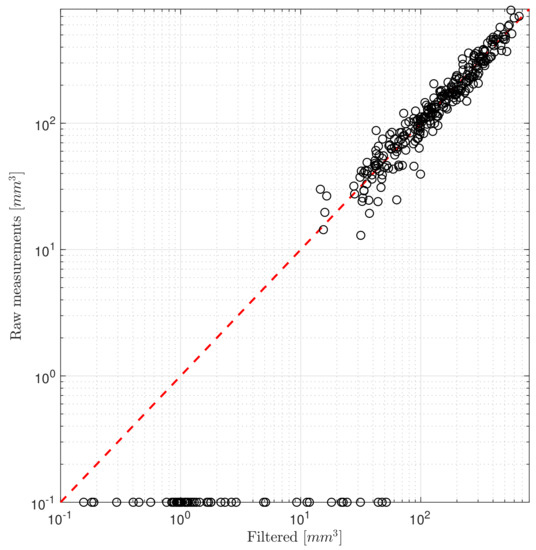
Figure 2.
Difference between the raw and filtered measurements.
The tumor volumes are measured using calipers and the actual volumes are approximated. This method is less accurate and reliable when smaller volumes are being measured. Data of measurements under 50 [mm] are rather scarce too, usually from a measured zero volume at the next sampling, the volume jumps instantly to the proximity of 50 [mm].
2.3.2. Kalman Filter Tuning
One critical aspect of comparing the performance of different observers is the tuning. In order to extract the most performance, the elements of the and covariance matrix were determined during an optimization. The goal of the optimization was to minimize the root-mean-square error (RMSE) between the measured trajectories and the predicted ones:
where N is the number of treated mice, is the vector of measured values of the i-th mouse and is the output of the system. The optimized parameters were in the main diagonal corresponding to the estimated parameters and the first element of the matrix to guarantee quicker convergence. The optimization is done by the function of the MATLAB environment from 100 initial points generated by the Latin Hypercube Sampling [18]. The optimized matrices are given as:
2.4. Moving Horizon Estimation
The MHE is an optimization-based method, where the minimization of a developed cost function is done on a moving window. A moving window of one step can coincide with the widely applied EKF. However, using a longer window and introducing some application-specific terms or constraints can be beneficial in several cases. Taking into account more measurements can result in an estimator more robust to external disturbances or delays.
The cost function can be formulated in several ways, depending on the application. General arguments and terms are summarized in Table 2, where the notations are given according to (4) and (5). The matrices provide weighting between the terms of the cost function, their subscripts indicates the analogy between the EKF and MHE. The weighting matrices are analogous to the inverses of the covariance matrices (8), (10). The vector function is the open-loop trajectory from the initial state of the current window, the arrival cost is calculated in the -th step, where M is the length of the horizon. The difference between the current parameters and the previous window is denoted by . Following the assumption that the mismatch between the model and measurements are caused by parameter uncertainty, intrapatient variability and measurement noise, the parameters are optimized, similarly to the EKF design. Given the arguments, the MHE problem can be generarly formulated as follows:
Table 2.
Moving horizon estimation (MHE) cost function formulations.
Compared to the general formulation, three modifications are implemented. First, as a worst case scenario the initial state of the horizon is set to the last estimated state. Secondly, the differences are normalized in order to make the weighting between the measurements and modifications easier, scaling the errors to the same order of magnitude. Division with zero is avoided: when the tumor volumes could not be exactly measured due to their small volumes, 1 [mm] is assigned to their measured value. Unit volume ensures numerical stability and is physiologically more relevant as the tumors are not completely eliminated. The charactheristics of the model is in agreement with this, as in ideal condition the volume converges to zero, but it is bound to be positive. Thirdly, a rational function (23) was introduced, which penalizes the difference less, when the measured tumor volumes are small. Justification for the second and third point is more detialed in Section 2.3.1. Considering these modifications the cost function in the k-th step is defined as
where is the sampling time of the measurements which is irregular; it varies between 1 and 5 days. This means that the sliding window shall also be irregular, so that when the new measurement is made, the window is adjusted to the time interval which is the closest to the predefined window length. Since the parameters are only modified when new measurements are made, the penalization of the change in parameter values can be different from time to time. In order to counteract this phenomenon, the parameter change penalization is normalized with the last sampling time. The upper and lower bounds for the parameters are defined as and . The bounds were introduced to be large to avoid saturation of variables during the simulation. According to our previous investigations, all four parameters remain in these regions during the model fitting regardless the measured volumes.
For the minimization of the cost function, the inbuilt function of the MATLAB software was applied. In each step, the initial values for the optimization were the estimates of the previous step which is often called hot start. In the first step, the initial values of the parameters are set to the nominal identified values from Table 1. Furthermore, the implementation of the cost function is extended with stopping criteria, rendering the optimization quicker or feasible at all. The intrinsic property of the model is that the tumor can grow even in cases when it is under treatment. It can occur that the optimizer selects parameter combinations which results in unrealistically large tumor volumes, thus making the solution of the differential equations unstable. To avoid such situations the propagation of such trajectories are stopped and penalized. The stopping threshold is based on clinical protocol, since the experiment has to be stopped, when the tumor volume grows larger 2000 [mm]. The cost is defined to be dependent on the volume, since otherwise assigning a constant value or infinity can make the optimizer stuck due to constant gradients of the object function. The change of parameter a is not penalized as it can be seen in (22). The reason behind this is that the tumor growth is dependent on the term. In the case of small tumor volumes, the model could not describe quickly varying tumor growth, unless more sudden changes are allowed for the a parameter. In the case of non-estimated parameters the nominal values were assigned from Table 1.
3. Results
The observers were evaluated on the data described in Section 2.1. As mentioned each mouse is labeled with PLD followed by an ID number. Estimation horizons of the MHE were tested in the 7–35 days range, however for better visibility only the 14 day version is shown beside the EKF.
Table 3 compares the RMSE of the measured and estimated volumes between the EKF and the investigated MHEs, given for each investigated mouse. When comparing the results two points must be emphasized. First, the assumptions made during the design of the observers. Secondly, the worst case scenario is investigated, in the sense that the EKF was tuned based on an optimization, where all the mice were taken into account. On the other hand, the weights of the MHE was not optimized only a penalizing function was introduced and applied instead of other tuning process. The RMSE indicates that for horizons shorter than 20 days the MHE can achieve better approximations on average. At horizon length of 28 days the results are varying from patient to patient. Only at 35 days the EKF has a clear edge over the MHE. Increasing the horizon of the MHE deteriorated the approximations as the actual parameter set had to describe longer sections, where structural mismatch and/or parameter variation occurs due to the change in the physiology of the tumor. At this point, it has to be emphasized again that while the MHE takes into account a series of measurements, the EKF works from sample to sample, thus various horizon lengths cannot be adapted.
Table 3.
RMSE between the measured and estimated volumes.
Figure 3 depicts the comparison of the time horizons using different measures. Three measures, namely mean absolute error (MAE), “noise” and standard deviation (SD) of each estimated parameter were selected in order to assess the performance of the observers and horizons. The MAE describes the general accuracy with respect to the measurements, the “noise” term quantifies the smoothness of the estimation by calculating the number of direction changes along the trajectory. The SD of each estimated parameter gives information about the range in which the parameter had to vary in order to provide an optimized fit. One can inspect that the MAE increases in a quasi-linear way with respect to the horizon. The smoothest trajectory is achieved by using 14-day-long horizon and the SD of parameter a is the lowest around 21 days. Concerning the penalized parameters b, w, n the lowest SD is achieved by using the 7-day-long horizon. The main difference between the EKF and MHE is that the optimization of the EKF resulted in very small gains for parameters a and n. This is anticipated as those parameters directly affect the tumor growth, with larger gains it may be possible to achieve better approximation for one patient, but it could lead to bigger divergence for a population. The divergence is avoided by the MHE as the optimization is constrained, parameter sets producing trajectories that reach 2000 [mm] are neglected.
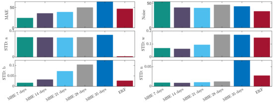
Figure 3.
Comparison of the investigated observers.
In Figure 4, an example (PLD ID:5) is given about the effect of the rational penalizing function. The function was introduced in (21). The two estimated trajectories, denoted by and are the output of the MHE with 14 days of horizon length. For visualization only the 14 day scenario is given, however, the effect is similar in the other cases, and the delay is more pronounced towards the longer horizons. It can be seen that without this weighting in the case of small volumes there is a significant delay in the response of the observer. The dashed purple lines show the value of the function with respect to time (, left subfigure) and the measured volume (, right subfigure).
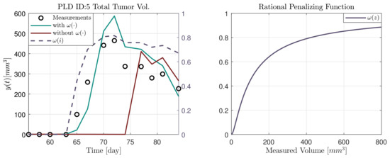
Figure 4.
Effect of the rational penalizing function.
In the following explanatory examples we address the problem of intrapatient variability, and how the observers were able to overcome it. Figure 5, Figure 6, Figure 7, Figure 8, Figure 9, Figure 10, Figure 11, Figure 12, Figure 13 and Figure 14. showcase the state and parameter estimations separately. The black circles denote the measurements, however, it is important to note that only the total tumor volume is measured, i.e., . The dashed magenta lines are the results from a Stochastic Approximation of Expectation-Maximization identification of the same model [6,7]. In the case of the , the three curves overlap, because parameters corresponding to (3) are not modified, hence nominal values were used. Those parameters are neglected in accordance with the previous sensitivity analysis [16]. Compared to the fixed identified parameter set by varying key parameters of the system, the observers are able to catch additional dynamics and track the measurements more accurately. This is particularly the case where the first administration of the chemotherapeutic drug made the tumor to shrink its volume close to zero. In fact, zero volumes were measured–namely, zero volumes are represented in the data–due to such small volumes cannot be measured accurately using calipers, albeit after a certain period of time, the tumor began to grow again. This phenomenon is observed in Figure 5 and Figure 7, where the identified sets could not model the first growth period. In Figure 9 the first growth occurs, but the discrepancy between the measurements and the model is still large. The even-numbered Figure 6, Figure 7, Figure 8, Figure 9 and Figure 10. show how the observers tackled the problem of tracking the first growth. It is particularly noticable in the case of the MHE, which started from a high growth rate (parameter a) and reduced it gradually to be able to maintain the tumor volume close to zero. Furthermore, it can be seen that the parameter a remains close to the identified value. However, at distinct time instances, greater divergence can be experienced. These divergences usually occur when the tumor exhibits a large growth rate. It can be observed that the identified models have a better fit when the tumor didn’t shrink to zero volumes after initial growth. This phenomena can be observed in Figure 11 and Figure 13.
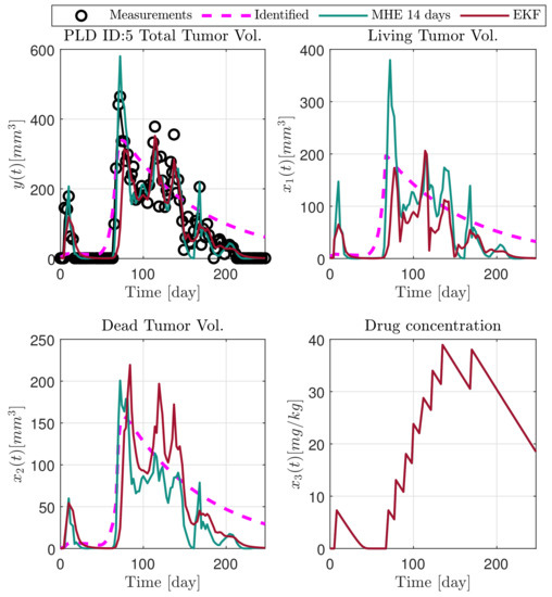
Figure 5.
Estimated states of PLD5 mouse.
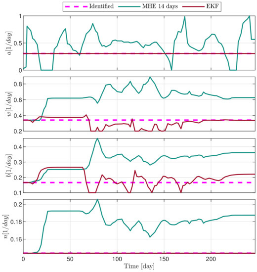
Figure 6.
Estimated parameters of PLD5 mouse.
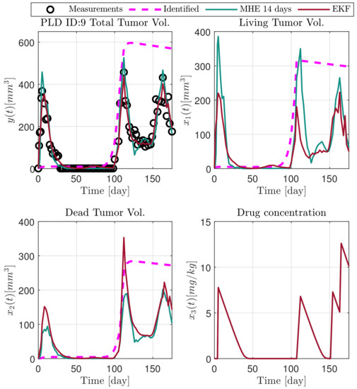
Figure 7.
Estimated states of PLD9 mouse.
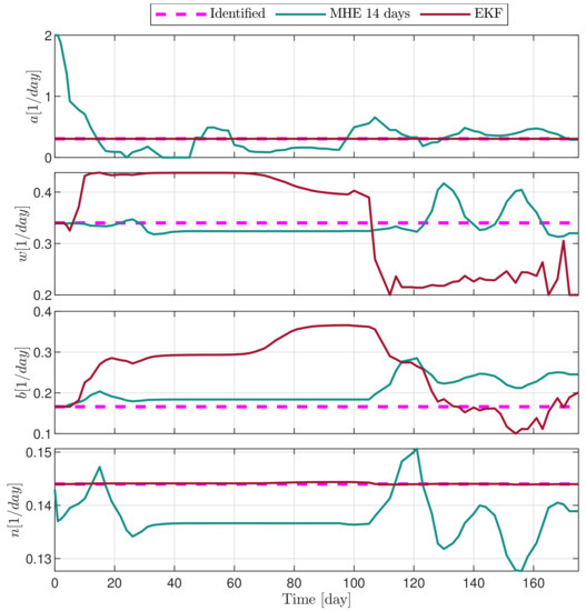
Figure 8.
Estimated parameters of PLD9 mouse.
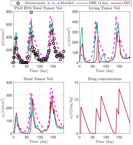
Figure 9.
Estimated states of PLD6 mouse.
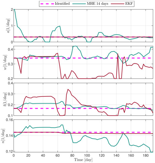
Figure 10.
Estimated parameters of PLD6 mouse.
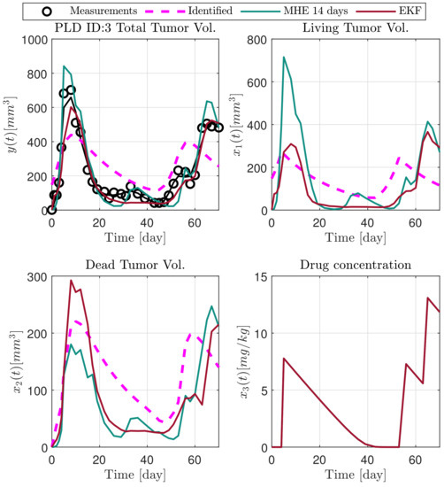
Figure 11.
Estimated states of PLD3 mouse.
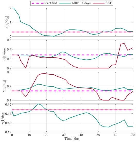
Figure 12.
Estimated parameters of PLD3 mouse.
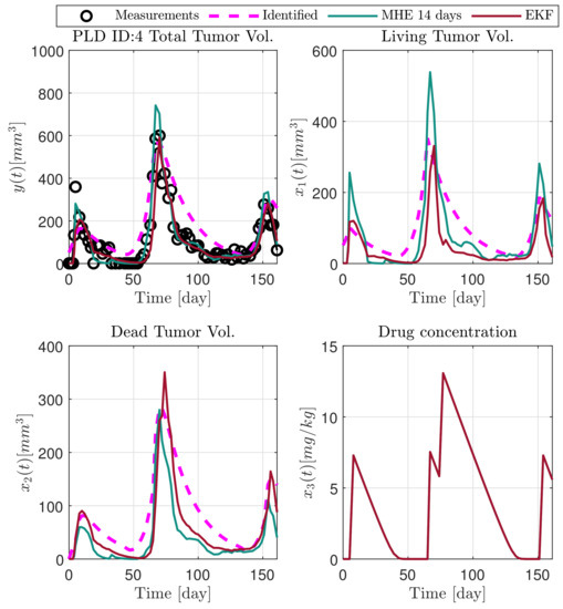
Figure 13.
Estimated states of PLD4 mouse.
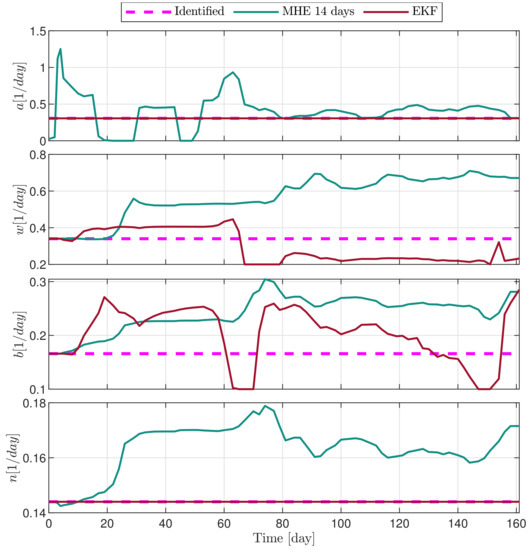
Figure 14.
Estimated parameters of PLD4 mouse.
4. Discussion
The goal was to evaluate the state and parameter estimation capabilities of an MHE and an EKF which has been applied as a benchmark. In general, state and parameter estimation in the case of physiological processes have major difficulties which are presented in this study related to tumor growth estimation as well. Furthermore, the problem formulation makes it even more difficult. In the model, only the sum of the living and dead tumor volumes can be measured, often inaccurately. This limited amount of data can easily lead to observability issues mostly coming from the fact that several state and parameter combinations may result in the same output. In order to limit these issues, we applied two key components: penalizing the velocity of changing of state variables and estimated parameters, moreover, we have selected a branch of key parameters to be estimated based on sensitivity analysis. Namely, the cost function of the MHE made it possible to use additional constraints and penalize the change of parameters. The penalization was designed to be close to the physiological rate of changes to be as as realisic as possible. According to the results, we have successfully limited the set of possible state and parameter sets leading to the same output without a downturn in the estimation accuracy.
The scenario for the comparison was designed to be biased arbitrary. The results show that even with optimizing the tuning of the EKF, and not taking into account the initial state of the MHE as an additional free variable, a moving horizon estimation based observer can still outperform the former EKF. The MHE-based observers achieved lower RMSE until the horizon length was shorter than 30 days. Using horizons around 20 days, there can be cases, where the EKF outperforms the MHE, e.g., the estimation of PLD9. At 7 days the difference in RMSE is around 30 [mm], and the MHE has lower RMSE for each mouse. The inferior performance of the EKF can rise from the low gains for parameters a and n. Since the system is most sensitive to those parameters, having larger gains could result in divergence in the case of certain patients due to the high interpatient variability. The estimation accuracy of the MHE deteriorated in a quasilinear manner with respect to the window length. The increased window lengths resulted in an increased RMSE of the tumor volumes because the effects of the structural mismatch became dominant. In general, a longer window would mean that the given parameter set is valid for more data. However, the predictive capabilities are crucial in therapy optimization, thus the determination of the optimal choice for closed-loop applications is future work. The runtime of the observers are greatly different. The EKF averages 2.6 ms, while the MHE ranges from 300 ms to 413 ms depending on the horizon length. However, runtime is not a cornerstone as the injections and measurements are done once a day at a maximum rate. An important aspect of the study is that the observers are evaluated on real laboratory data, where two major difficulties are present: structural mismatch and intrapatient variability.
The results indicate the great importance of applying observers for therapy optimization algorithms. Without constant feedback about the behavior of the patient the model using only a single parameter set can introduce large discrepancies. As the tumor shifts phases, and as the heterogenity of the tumor changes its behavior changes as well. These shifts in physiology can be tracked with the observers–particularly well with the MHE–. These changes can be interpreted as trends in the parameters. Additionally, despite the optimized tuning of the EKF the MHE shows a smoother estimation of the parameters and a more accurate approximation of the measurements. These attributes facilitate the application of the MHE in closed-loop algorithms.
5. Conclusions
In this paper, an MHE-based observer and an EKF was designed and compared for therapy optimization and state-feedback kind of control applications. When using time horizons less than 28 days, the MHE based observer had superior performance—compared to the EKF—in tracking the measurements. Increased horizon length deteriorated the approximations as the actual parameter set had to describe longer sections, where structural mismatch and/or parameter variation occurs due to the change in the physiology of the tumor. To evaluate the performance more thoroughly advanced measurement technology is needed to distinguish live and dead tumor cells and even drug concentration. Further improvements can be done on the fine-tuning of the parameters in the cost function. Future work includes the integration of the MHE into closed-loop systems.
Author Contributions
Conceptualization, M.S., G.E., D.A.D. and L.K.; methodology, M.S., G.E., D.A.D.; writing—original draft preparation, M.S., G.E.; writing—review and editing, M.S., G.E., D.A.D., I.R., L.K.; supervision, G.E., D.A.D., L.K. All authors have read and agreed to the published version of the manuscript.
Funding
This project has received funding from the European Research Council (ERC) under the European Union’s Horizon 2020 research and innovation programme (grant agreement No 679681). Project no. 2019-1.3.1-KK-2019-00007. has been implemented with the support provided from the National Research, Development and Innovation Fund of Hungary, financed under the 2019-1.3.1-KK funding scheme. M. Siket was supported by the ÚNKP-19-3 and ÚNKP-20-3 New National Excellence Program of the Ministry for Innovation and Technology.
Acknowledgments
The Authors would like to thank to András Füredi and Gergő Szakács from the Membrane Protein Research Group of the Research Centre for Natural Sciences for providing the experimental data and the many useful advices they made. The Authors would also like to thank the support of the Applied Informatics and Applied Mathematics Doctoral School.
Conflicts of Interest
The authors declare no conflict of interest.
Ethical Statement
The data of animal experiments has been provided by the Membrane Protein Research Group of the Research Centre for Natural Sciences. In this project, approval of any ethical committee has not been necessary.
Abbreviations
The following abbreviations are used in this manuscript:
| EKF | Extended Kalman filter |
| MHE | moving horizon estimation |
| RMSE | root-mean-square error |
References
- WHO: Cancer. Available online: https://www.who.int/news-room/fact-sheets/detail/cancer (accessed on 11 March 2020).
- Ren, H.P.; Yang, Y.; Baptista, M.S.; Grebogi, C. Tumour chemotherapy strategy based on impulse control theory. Philos. Trans. Math. Phys. Eng. Sci. 2017, 375. [Google Scholar] [CrossRef] [PubMed]
- Drexler, D.A.; Ferenci, T.; Kovács, L. Extended tumor growth model for combined therapy. In Proceedings of the 2019 IEEE International Conference on Systems, Man and Cybernetics (SMC), Bari, Italy, 6–9 October 2019; pp. 886–891. [Google Scholar] [CrossRef]
- Hahnfeldt, P.; Panigrahy, D.; Folkman, J.; Hlatky, L. Tumor Development under Angiogenic Signaling. Cancer Res. 1999, 59, 4770. [Google Scholar] [PubMed]
- d’Onofrio, A.; Gandolfi, A. Tumour eradication by antiangiogenic therapy: Analysis and extensions of the model by Hahnfeldt et al. (1999). Math. Biosci. 2004, 191, 159–184. [Google Scholar] [CrossRef] [PubMed]
- Drexler, D.A.; Ferenci, T.; Lovrics, A.; Kovács, L. Modeling of tumor growth incorporating the effect of pegylated liposomal doxorubicin. In Proceedings of the 2019 IEEE 23nd International Conference on Intelligent Engineering Systems, Gödöllő, Hungary, 25–27 April 2019; pp. 369–373. [Google Scholar]
- Drexler, D.A.; Ferenci, T.; Lovrics, A.; Kovács, L. Tumor dynamics modeling based on formal reaction kinetics. Acta Polytech. Hung. 2019, 16, 31–44. [Google Scholar] [CrossRef]
- Kuznetsov, M.; Kolobov, A. Investigation of solid tumor progression with account of proliferation/migration dichotomy via Darwinian mathematical model. J. Math. Biol. 2020, 80. [Google Scholar] [CrossRef] [PubMed]
- Kuznetsov, M. Mathematical Modeling Shows That the Responseof a Solid Tumor to Antiangiogenic TherapyDepends on the Type of Growth. Mathematics 2020, 8, 760. [Google Scholar] [CrossRef]
- Rokhforoz, P.; Jamshidi, A.A.; Sarvestani, N.N. Adaptive robust control of cancer chemotherapy with extended Kalman filter observer. Inform. Med. Unlocked 2017, 8, 1–7. [Google Scholar] [CrossRef]
- Costa, J.M.; Orlande, H.R.; Velho, H.F.C.; de Pinho, S.T.; Dulikravich, G.S.; Cotta, R.M.; da Cunha Neto, S.H. Estimation of Tumor Size Evolution Using Particle Filters. J. Comput. Biol. 2015, 22, 649–665. [Google Scholar] [CrossRef] [PubMed]
- Sápi, J.; Drexler, D.; Harmati, I.; Sápi, Z.; Kovács, L. Qualitative analysis of tumor growth model under antiangiogenic therapy—Choosing the effective operating point and design parameters for controller design. Optim. Control Appl. Methods 2016, 37, 848–866. [Google Scholar] [CrossRef]
- Chen, T.; Kirkby, N.; Jena, R. Optimal dosing of cancer chemotherapy using model predictive control and moving horizon state/parameter estimation. Comput. Methods Programs Biomed. 2012, 108. [Google Scholar] [CrossRef] [PubMed]
- Füredi, A.; Szebényi, K.; Tóth, S.; Cserepes, M.; Hámori, L.; Nagy, V.; Karai, E.; Vajdovich, P.; Imre, T.; Szabó, P.; et al. Pegylated liposomal formulation of doxorubicin overcomes drug resistance in a genetically engineered mouse model of breast cancer. J. Control Release 2017, 261, 287–296. [Google Scholar] [CrossRef] [PubMed]
- Drexler, D.A.; Nagy, I.; Romanovski, V.; Tóth, J.; Kovács, L. Qualitative analysis of a closed-loop model of tumor growth control. In Proceedings of the 18th IEEE International Symposium on Computational Intelligence and Informatics, Budapest, Hungary, 21–22 November 2018; pp. 329–334. [Google Scholar]
- Siket, M.; Eigner, G.; Kovács, L. Sensitivity and identifiability analysis of a third-order tumor growth model. In Proceedings of the IEEE 15th International Conference on System of Systems Engineering, Budapest, Hungary, 2–4 June 2020. [Google Scholar]
- Villaverde, A.F.; Barreiro, A. Identifiability of Large Nonlinear Biochemical Networks. MATCH Commun. Math. Comput. Chem. 2016, 96, 259–296. [Google Scholar]
- Iman, R.L. Latin Hypercube Sampling. In Wiley StatsRef: Statistics Reference Online; American Cancer Society: Atlanta, GA, USA, 2014. [Google Scholar] [CrossRef]
Publisher’s Note: MDPI stays neutral with regard to jurisdictional claims in published maps and institutional affiliations. |
© 2020 by the authors. Licensee MDPI, Basel, Switzerland. This article is an open access article distributed under the terms and conditions of the Creative Commons Attribution (CC BY) license (http://creativecommons.org/licenses/by/4.0/).