Determination of the Operating Temperature of the Gas-Insulated Transmission Line ^†

Abstract

Gas-insulated lines (GILs) have been increasingly used as high-current busducts for high-power transmission. Temperature is one of the most important factors affecting the performance and ampacity of GILs. In this paper, an analytical method was proposed to determine the temperature of a three-phase high-current busduct in the form of a single pole GIL. First, power losses in the phase conductors and enclosures were determined analytically with the skin, and proximity effects were taken into account. The determined power losses were used as heat sources in thermal analysis. Considering the natural convection and radiation heat transfer effects, the heat balance equations on the surface of the phase conductors and the screens were established, respectively. Subsequently, the temperature of the phase conductors and the enclosures were determined. The validation of the proposed method was carried out using the finite element method and laboratory measurements.

1. Introduction

The growing demand for electrical energy requires a continuous expansion of the electric power infrastructure. Today, it has become increasingly popular to generate electricity in distributed energy sources, both on photovoltaic farms and in small co-generation units. Large-scale wind power plants or photovoltaic farms are usually far away from load centers and need to be connected with an electric power grid. The installation of the overhead lines is not possible everywhere, especially in cities or across seas; therefore, underground solutions for electric energy transmission are needed. Almost 50 years of using gas-insulated lines (GILs) in electric power infrastructure make them good candidates to be used as high-power underground transmission systems [1,2,3,4,5,6,7,8].

GILs were introduced to power engineering in the late 1960s and are widely used today with high reliability. High-current GILs were often used in power generation and substation facilities as power transmission lines. Their main area of application is as a connection between the generator unit and its step-up transformer. Today, GILs are applied in many projects around the world where high-powered transmission with high reliability and maximum availability is required. The sizes of the projects are constantly increasing: from system lengths of a few meters, in the past, to several dozen kilometers, today. High-current busduct systems are usually gas insulated single-pole systems and tubular aluminum or copper conductors encapsulated in the coaxial aluminum screen. The insulating medium in the first generation of GILs was SF₆ (sulfur hexafluoride) under pressures ranging from 0.29 to 0.51 MPa (at 20 °C). In the next generation of GILs, SF₆ has been replaced with a mixture of nitrogen and SF₆. The operation pressure is dependent on the mixture temperature and is specific in particular installations. Due to environmental protection requirements, the mixture of N₂ and SF₆ is preferred in applications where large gas quantities are used and where dielectric performance is desired [9,10,11,12,13,14,15,16,17,18,19,20].

The simple design of GILs has proven to be highly reliable over the last 50 years of operation. Until recently, no critical failure has been reported from any installation in the world [18]. GILs have several advantages, such as low transmission losses and high transmission efficiency, low capacitive load, low electromagnetic field, high reliability, no electric and thermal aging, low environmental influence and a high level of safety concerning surrounding equipment or nearby personnel [21,22,23,24,25,26,27,28,29,30,31].

GIL technology is increasingly becoming popular in the bulk transmission of electric power across long distances. The high-current busducts can be installed above ground, in a tunnel, trench or directly buried. These installation opportunities offer a large field of possible applications inside substations and power plants or even outside as cross-country installations. The simple design and high safety level of GILs allows for their installation in traffic and railway tunnels [7,8,18,19,20].

GILs can be installed in a street or railroad tunnel because they do not pose a threat to other users or elements of the tunnel. They can also be fixed on the tunnel roof or laid in a separate tunnel, which is often used as an emergency exit tunnel. Moreover, GILs low capacitive load makes it possible to build busducts lengths of up to 800 km without any reactive power compensation. For these reasons, very long tunnel systems can also be equipped with GILs [18].

The use of traffic tunnels with GILs is now under investigation in different parts of the world. In Europe, interconnections between Germany, Austria, Switzerland, Italy and France are planned to improve the traffic flow and to allow trade of electrical energy. In Asia, especially in China and Indonesia, interconnections between the mainland and islands are under investigation [7,8,18,19,20].

Today, overhead lines are the most economical means of high-voltage transmission, but in the near future, due to environmental protection requirements, GIL technology could replace conventional cables and overhead lines and will be widely used in long distance transmission lines [7,8,18].

The design of GILs for high-current and voltage use requires precise analysis of electromagnetic, dynamic and thermal effects. The knowledge of the relationship between electrodynamics and constructional parameters is crucial during the design and optimization process of high-current busducts [3,7,8,16,24,25]. The temperature rise of a gas-insulated line is a vital factor that has an adverse effect on its performance. Exceeding the permissible temperature level leads to damage of the transmission line and, often, to the loss of all the components connected to it. One of the most important parameters of a high-current busduct is its ampacity, i.e., the maximum current that can be carried without exceeding its temperature rating [16,17]. Power losses and the temperature depend on the value of the currents, and, for the large cross-sectional dimensions of phase conductors and screens, even at an industrial frequency, the skin effect as well as the external and internal proximity effects should be taken into account [24,25,29].

In the last three decades, the prediction of the operating temperature of high-current busducts has been the subject of a number of investigations [7,8]. Most of them deal with specific busduct configurations [4,5,10,12,13,14,15,17,27,28,31]. The heating of busducts has been studied both numerically and experimentally. In many cases, the problem has been formulated as a magneto-thermal one, linking the busduct ampacity with the operating temperature [5,9,10,11,21,22,28]. In this contribution, an analytical method to determine the temperature of a tubular high-current busduct with isolated phases was proposed. First, the power losses in the phase conductors and screens were determined. In the next step, the temperature rise of the phase conductors and screens were calculated by solving the thermal equilibrium equations. In the calculation of power losses, the skin and proximity effects were taken into account.

2. Magneto-Thermal Modeling

Let us consider the operating temperature of the three-phase high-current busduct presented in Figure 1.

At a steady state, the heat generated and dissipated in the three-phase high-current busduct satisfies the following equations [12,13,28]:

$$P=Q_C+Q_R$$

(1)

$$P+P_e=Q_{eC}+Q_{eR}$$

(2)

where P and P_e are the power losses in the phase conductor and in the enclosure, respectively, Q_C and Q_eC are the convection heat transfer of the phase conductor and the enclosure, respectively, and Q_R and Q_eR are the radiation heat transfer of the phase conductor and the enclosure, respectively.

For the phase conductor, the convection and radiation heat transfer are [12,13,28]

$$Q_C=\frac{T-T_o}{\frac{1}{2\pi \alpha R_2}+\frac{1}{2\pi \lambda }\ln \frac{R_3}{R_2}+\frac{1}{2\pi \alpha R_3}}$$

(3)

$$Q_R=2{\sigma }_o{\epsilon }_n\pi R_2\left({\left(\frac{T}{100}\right)}^4-{\left(\frac{T_e}{100}\right)}^4\right)$$

(4)

where T and T_e are the temperatures of the phase conductor and the enclosure, respectively, T_o is the ambient temperature, λ is the thermal conductivity of the phase conductor, α is the convective heat transfer coefficient of the phase conductor, ${\sigma }_o=5.67·{10}^{-8}\left[\frac{\mathrm{W}}{{\mathrm{m}}^2{\mathrm{K}}^4}\right]$ is the Stefan–Boltzmann constant and ε_n is emissivity, which can be calculated from the following equation [12]:

$${\epsilon }_n=\frac{1}{\frac{1}{\epsilon }+\frac{R_2}{R_3}\left(\frac{1}{{\epsilon }_e}-1\right)}$$

(5)

in which ε is an emissivity of the phase conductor and ε_e is an emissivity of the enclosure.

The convection and radiation heat transfer of the enclosure is [28]

$$Q_{eC}=2\pi {\alpha }_e{R}_4\left(T_e-T_o\right)$$

(6)

$$Q_{eR}=2{\sigma }_o{\epsilon }_e\pi R_4\left({\left(\frac{T_e}{100}\right)}^4-{\left(\frac{T_o}{100}\right)}^4\right)$$

(7)

where α_e is the convective heat transfer coefficient of the enclosure.

Power losses in the conductors of the single-pole high-current busduct presented in Figure 1 are expressed by formula [29]

$$P_{}=\frac{ \underset{¯}{\Gamma } l I_1^2}{4 \pi \gamma R_2} \frac{\underset{¯}{a}}{ \underset{¯}{b} {\underset{¯}{b}}^{\ast } }$$

(8)

where

$$\underset{¯}{b}=I_1\left(\underset{¯}{\Gamma } R_2\right) K_1\left(\underset{¯}{\Gamma } R_1\right)-I_1\left(\underset{¯}{\Gamma } R_1\right) K_1\left(\underset{¯}{\Gamma } R_2\right)$$

(9)

$${\underset{¯}{b}}^{\ast }=I_1^{\ast }\left(\underset{¯}{\Gamma } R_2\right) K_1^{\ast }\left(\underset{¯}{\Gamma } R_1\right)-I_1^{\ast }\left(\underset{¯}{\Gamma } R_1\right) K_1^{\ast }\left(\underset{¯}{\Gamma } R_2\right)$$

(10)

and

$$\begin{array}{ll}\underset{¯}{a}& =K_1(\underset{¯}{\Gamma }{R}_1) K_1^{\ast }(\underset{¯}{\Gamma }{R}_1) \left[I_0(\underset{¯}{\Gamma }{R}_2) I_1^{\ast }(\underset{¯}{\Gamma }{R}_2)-\mathrm{j} I_1(\underset{¯}{\Gamma }{R}_2) I_0^{\ast }(\underset{¯}{\Gamma }{R}_2)\right]\\ & -I_1(\underset{¯}{\Gamma }{R}_1) I_1^{\ast }(\underset{¯}{\Gamma }{R}_1)\left[K_0(\underset{¯}{\Gamma }{R}_2) K_1^{\ast }(\underset{¯}{\Gamma }{R}_2)-\mathrm{j} K_1(\underset{¯}{\Gamma }{R}_2) K_0^{\ast }(\underset{¯}{\Gamma }{R}_2)\right]\\ & +I_1(\underset{¯}{\Gamma }{R}_1) K_1^{\ast }(\underset{¯}{\Gamma }{R}_1)\left[K_0(\underset{¯}{\Gamma }{R}_2) I_1^{\ast }(\underset{¯}{\Gamma }{R}_2)+\mathrm{j} K_1(\underset{¯}{\Gamma }{R}_2) I_0^{\ast }(\underset{¯}{\Gamma }{R}_2)\right]\\ & -K_1(\underset{¯}{\Gamma }{R}_1) I_1^{\ast }(\underset{¯}{\Gamma }{R}_1)\left[I_0(\underset{¯}{\Gamma }{R}_2) K_1^{\ast }(\underset{¯}{\Gamma }{R}_2)+\mathrm{j} I_1(\underset{¯}{\Gamma }{R}_2) K_0^{\ast }(\underset{¯}{\Gamma }{R}_2)\right]\end{array}$$

(11)

In the above formulas, $I_0(\underset{¯}{\Gamma }r)$, $K_0(\underset{¯}{\Gamma }r)$, $I_1(\underset{¯}{\Gamma }{R}_1)$, $K_1(\underset{¯}{\Gamma }{R}_1)$ and $I_1(\underset{¯}{\Gamma }{R}_2)$, $K_1(\underset{¯}{\Gamma }{R}_2)$ are the modified Bessel functions of the first and second kind and order 0 or 1 [32] and the Γ is the complex propagation constant in the phase conductor:

$$\underset{¯}{\Gamma }=\sqrt{\mathrm{j}\omega {\mathsf{\mu }}_0\gamma }=k+\mathrm{j}k$$

(12)

in which k is the attenuation constant

$$k=\sqrt{\frac{\omega {\mathsf{\mu }}_0\gamma }{2}}=\frac{1}{\delta }$$

(13)

where δ is the electrical skin depth of the electromagnetic wave penetration into the conducting environment, ω is the angular frequency, $\gamma$ stands for the electrical conductivity of the phase conductor and ${\mathsf{\mu }}_0=4\pi {10}^{-7} \mathrm{H}·{\mathrm{m}}^{-1}$ is the magnetic permeability of the vacuum.

In turn, power losses in the outer screens (E1 and E3) were almost the same and can be written down as follows [29]:

$$P_{s13}=P_{e0}+P_{e13}$$

(14)

where

$$P_{\mathrm{e}0}=\frac{{\underset{¯}{\Gamma }}_{\mathrm{e}}^{*} l I_1^{}{}^2}{{4 \mathsf{\pi } \mathsf{\gamma }}_{\mathrm{e}} {\beta }_{\mathrm{e}}^2 R_4}\frac{{\underset{¯}{a}}_0}{{\underset{¯}{d}}_0 {\underset{¯}{d}}_0^{*}}$$

(15)

in which

$$\begin{array}{ll}{\underset{¯}{a}}_0& ={\underset{¯}{b}}_0 {\underset{¯}{b}}_0^{*}\left\{I_0^{*}({\underset{¯}{\Gamma }}_{\mathrm{e}}{R}_4)I_1({\underset{¯}{\Gamma }}_{\mathrm{e}}{R}_4)+\mathrm{j} I_0({\underset{¯}{\Gamma }}_{\mathrm{e}}{R}_4)I_1^{*}({\underset{¯}{\Gamma }}_{\mathrm{e}}{R}_4)-{\beta }_{\mathrm{e}}\left[I_0^{*}({\underset{¯}{\Gamma }}_{\mathrm{e}}{R}_3)I_1({\underset{¯}{\Gamma }}_{\mathrm{e}}{R}_3)+\mathrm{j} I_0({\underset{¯}{\Gamma }}_{\mathrm{e}}{R}_3)I_1^{*}({\underset{¯}{\Gamma }}_{\mathrm{e}}{R}_3)\right]\right\}\\ & -{\underset{¯}{c}}_0 {\underset{¯}{c}}_0^{*}\left\{K_0^{*}({\underset{¯}{\Gamma }}_{\mathrm{e}}{R}_4)K_1({\underset{¯}{\Gamma }}_{\mathrm{e}}{R}_4)+\mathrm{j} K_0({\underset{¯}{\Gamma }}_{\mathrm{e}}{R}_4)K_1^{*}({\underset{¯}{\Gamma }}_{\mathrm{e}}{R}_4)-{\beta }_{\mathrm{e}}\left[K_0^{*}({\underset{¯}{\Gamma }}_{\mathrm{e}}{R}_3)K_1({\underset{¯}{\Gamma }}_{\mathrm{e}}{R}_3)+\mathrm{j} K_0({\underset{¯}{\Gamma }}_{\mathrm{e}}{R}_3)K_1^{*}({\underset{¯}{\Gamma }}_{\mathrm{e}}{R}_3)\right]\right\}\\ & -{\underset{¯}{c}}_0 {\underset{¯}{b}}_0^{*}\left\{I_0^{*}({\underset{¯}{\Gamma }}_{\mathrm{e}}{R}_4)K_1({\underset{¯}{\Gamma }}_{\mathrm{e}}{R}_4)-\mathrm{j} K_0({\underset{¯}{\Gamma }}_{\mathrm{e}}{R}_4)I_1^{*}({\underset{¯}{\Gamma }}_{\mathrm{e}}{R}_4)-{\beta }_{\mathrm{e}}\left[I_0^{*}({\underset{¯}{\Gamma }}_{\mathrm{e}}{R}_3)K_1({\underset{¯}{\Gamma }}_{\mathrm{e}}{R}_3)-\mathrm{j} K_0({\underset{¯}{\Gamma }}_{\mathrm{e}}{R}_3)I_1^{*}({\underset{¯}{\Gamma }}_{\mathrm{e}}{R}_3)\right]\right\}\\ & +{\underset{¯}{b}}_0 {\underset{¯}{c}}_0^{*}\left\{I_1({\underset{¯}{\Gamma }}_{\mathrm{e}}{R}_4)K_0^{*}({\underset{¯}{\Gamma }}_{\mathrm{e}}{R}_4)-\mathrm{j} I_0({\underset{¯}{\Gamma }}_{\mathrm{e}}{R}_4)K_1^{*}({\underset{¯}{\Gamma }}_{\mathrm{e}}{R}_4)-{\beta }_{\mathrm{e}}\left[I_1({\underset{¯}{\Gamma }}_{\mathrm{e}}{R}_3)K_0^{*}({\underset{¯}{\Gamma }}_{\mathrm{e}}{R}_3)-\mathrm{j} I_0({\underset{¯}{\Gamma }}_{\mathrm{e}}{R}_3)K_1^{*}({\underset{¯}{\Gamma }}_{\mathrm{e}}{R}_3)\right]\right\}\end{array}$$

(16)

$${\underset{¯}{b}}_0={\beta }_e K_1({\underset{¯}{\Gamma }}_e{R}_3)-K_1({\underset{¯}{\Gamma }}_e{R}_4)$$

(17)

$${\underset{¯}{b}}_0^{*}={\beta }_{\mathrm{e}} K_1^{*}({\underset{¯}{\Gamma }}_{\mathrm{e}}{R}_3)-K_1^{*}({\underset{¯}{\Gamma }}_{\mathrm{e}}{R}_4)$$

(18)

$${\underset{¯}{c}}_0={\beta }_e I_1({\underset{¯}{\Gamma }}_e{R}_3)-I_1({\underset{¯}{\Gamma }}_e{R}_4)$$

(19)

$${\underset{¯}{c}}_0^{*}={\beta }_{\mathrm{e}} I_1^{*}({\underset{¯}{\Gamma }}_{\mathrm{e}}{R}_3)-I_1^{*}({\underset{¯}{\Gamma }}_{\mathrm{e}}{R}_4)$$

(20)

$${\underset{¯}{d}}_0=I_1({\underset{¯}{\Gamma }}_e{R}_4) K_1({\underset{¯}{\Gamma }}_e{R}_3)-I_1({\underset{¯}{\Gamma }}_e{R}_3) K_1({\underset{¯}{\Gamma }}_e{R}_4)$$

(21)

$${\underset{¯}{d}}_0^{*}=I_1^{*}({\underset{¯}{\Gamma }}_{\mathrm{e}}{R}_4)K_1^{*}({\underset{¯}{\Gamma }}_{\mathrm{e}}{R}_3)- I_1^{*}({\underset{¯}{\Gamma }}_{\mathrm{e}}{R}_3)K_1^{*}({\underset{¯}{\Gamma }}_{\mathrm{e}}{R}_4)$$

(22)

$${\beta }_e=\frac{R_3}{R_4} ( 0\le {\beta }_e\le 1)$$

(23)

Power P_e13 has a following form

$$P_{e13}=\frac{{\underset{¯}{\Gamma }}_e{}^{*} l I_1^2}{2 \pi \gamma R_4}{\displaystyle \sum _{n=1}^{\infty }{A}_n^2 {\left(\frac{R_4}{d}\right)}^{2n}\frac{{\underset{¯}{a}}_{ne}}{{\underset{¯}{b}}_{ne} {\underset{¯}{b}}_{ne}^{*}}}$$

(24)

where

$${\underset{¯}{A}}_n=-\frac{1}{2}\left[\left(1+2^{-n}\right)+\mathrm{j} \sqrt{3} \left(1-2^{-n}\right)\right]=A_n \exp [\mathrm{j} {\phi }_n]$$

(25)

$${\underset{¯}{b}}_{ne}=I_{n-1}({\underset{¯}{\Gamma }}_e{R}_4) K_{n+1}({\underset{¯}{\Gamma }}_e{R}_3)-I_{n+1}({\underset{¯}{\Gamma }}_e{R}_3) K_{n-1}({\underset{¯}{\Gamma }}_e{R}_4)$$

(26)

$${\underset{¯}{b}}_{ne}^{*}=I_{n-1}^{*}({\underset{¯}{\Gamma }}_e{R}_4) K_{n+1}^{*}({\underset{¯}{\Gamma }}_e{R}_3)-I_{n+1}^{*}({\underset{¯}{\Gamma }}_e{R}_3) K_{n-1}^{*}({\underset{¯}{\Gamma }}_e{R}_4)$$

(27)

$$\begin{array}{ll}{\underset{¯}{a}}_{ne}& =I_{n+1}({\underset{¯}{\Gamma }}_e{R}_4) K_{n+1}({\underset{¯}{\Gamma }}_e{R}_3) \left[I_{n+1}^{*}({\underset{¯}{\Gamma }}_e{R}_3) K_n^{*}({\underset{¯}{\Gamma }}_e{R}_4)+I_n^{*}({\underset{¯}{\Gamma }}_e{R}_4) K_{n+1}^{*}({\underset{¯}{\Gamma }}_e{R}_3) \right]\\ & +\mathrm{j} I_n({\underset{¯}{\Gamma }}_e{R}_4) K_{n+1}({\underset{¯}{\Gamma }}_e{R}_3) \left[I_{n+1}^{*}({\underset{¯}{\Gamma }}_e{R}_4) K_{n+1}^{*}({\underset{¯}{\Gamma }}_e{R}_3) -I_{n+1}^{*}({\underset{¯}{\Gamma }}_e{R}_3) K_{n+1}^{*}({\underset{¯}{\Gamma }}_e{R}_4) \right]\\ & -I_{n+1}({\underset{¯}{\Gamma }}_e{R}_3)K_{n+1}^{*}({\underset{¯}{\Gamma }}_e{R}_3) \left[I_n^{*}({\underset{¯}{\Gamma }}_e{R}_4) K_{n+1}({\underset{¯}{\Gamma }}_e{R}_4)- \mathrm{j} I_{n+1}^{*}({\underset{¯}{\Gamma }}_e{R}_4) K_n({\underset{¯}{\Gamma }}_e{R}_4)\right]\\ & -I_{n+1}({\underset{¯}{\Gamma }}_e{R}_3)I_{n+1}^{*}({\underset{¯}{\Gamma }}_e{R}_3)\left[K_n^{*}({\underset{¯}{\Gamma }}_e{R}_4) K_{n+1}({\underset{¯}{\Gamma }}_e{R}_4)+ \mathrm{j} K_{n+1}^{*}({\underset{¯}{\Gamma }}_e{R}_4) K_n(\underset{¯}{\Gamma }{R}_4)\right]\end{array}$$

(28)

Power losses in the middle screen (E2) are [29]

$$P_{s2}=P_{e0}+P_{e2}$$

(29)

where

$$P_{e2}=\frac{{\underset{¯}{\Gamma }}_e{}^{*} l I_1^2}{2 \pi \gamma R_4}{\displaystyle \sum _{n=1}^{\infty }{B}_n^2 {\left(\frac{R_4}{d}\right)}^{2n}\frac{{\underset{¯}{a}}_{ne}}{{\underset{¯}{b}}_{ne} {\underset{¯}{b}}_{ne}^{*}}}$$

(30)

and

$${\underset{¯}{B}}_n=\frac{1}{2}\left\{-\left[{\left(-1\right)}^n+1\right]+\mathrm{j} \sqrt{3} \left[{\left(-1\right)}^n-1\right]\right\}=B_n \exp [\mathrm{j} {\psi }_n]$$

(31)

In the thermal analysis, the material properties, such as electrical conductivity, are temperature-dependent; therefore, nonlinear thermal analysis was performed. The electrical conductivity can be expressed by the following equation [33]:

$$\gamma =\frac{{\gamma }_{20}}{1+{\alpha }_{20}(T-20)}$$

(32)

where: ${\gamma }_{20}$ is the electrical conductivity at 20 °C and ${\alpha }_{20}$ is the temperature coefficient.

The heat generated in the high-current busduct is transferred to the ambient air by natural convection and radiation on the internal surface of the enclosure. Therefore, the total heat transfer coefficient α is a sum of the radiation α_r and convection α_c heat transfer coefficient. If radiation heat flow occurs between two surfaces F1 and F2, then the radiation heat transfer coefficient can be calculated by [33]:

$${\alpha }_r={\phi }_{F1,F2}{\sigma }_0\frac{T_{F1}^4-T_{F2}^4}{T_{F1}^{}-T_{F2}^{}}$$

(33)

where φ_F,F1 is a configuration coefficient of surfaces F1 and F2. The configuration coefficient depends on the shape and the mutual location of the surfaces. In the case of the tubular high-current busduct, surface F1 is placed concentric to surface F2 (Figure 2).

For the case presented in Figure 2, the configuration coefficient φ_F1,F2 can be calculated using the following equation [33]:

$${\phi }_{F1,F2}=\frac{1}{\frac{1}{{\epsilon }_1}+\frac{F1}{F2}\left(\frac{1}{{\epsilon }_2}-1\right)}$$

(34)

where

• F1 is the area of the outer phase conductor surface,
• F2 is the area of the inner enclosure surface,
• ε₁ is the emissivity of the surface F1 and
• ε₂ is the emissivity of the surface F2.

The convection heat transfer coefficient α_c can be determined using the similarity theory and non-dimensional parameters, including the Grashof (Gr), Prandtl (Pr), Rayleigh (Ra) and Nusselt (Nu) numbers [28,33]. The Nusselt number, Nu, for the two concentric cylinders can be defined by the following equation [33]:

$${\mathrm{Nu}}_m=C·{\mathrm{Ra}}_m^n$$

(35)

The Rayleigh number, Ra, can be expressed as

$$\mathrm{Ra}=\mathrm{Pr}·\mathrm{Gr}$$

(36)

where the Prandtl, Pr, number is given by the following equation

$$\mathrm{Pr}=\frac{\eta ·c_p}{\lambda }$$

(37)

and the Grashof number, Gr, has a form as follows:

$$\mathrm{Gr}=\frac{g·\beta ·\Delta T·l^3}{{\nu }^2}$$

(38)

In Equations (35)–(38), g denotes the gravitational acceleration, β is the coefficient of thermal expansion, l is the equivalent linear dimension, ν is the kinematic viscosity, η is the dynamic viscosity, c_P is the specific heat, $\Delta T$ is the temperature difference and C and n are dimensionless constants dependent on the system (

Table 1. Coefficients C and n for the horizontal cylinders [33].

Range of Applicability	C	n
${10}^{-10}<{\mathrm{Ra}}_m\le {10}^{-2}$	0.675	0.058
${10}^{-2}<{\mathrm{Ra}}_m\le {10}^2$	1.020	0.148
${10}^2<{\mathrm{Ra}}_m\le {10}^4$	0.850	0.188
${10}^4<{\mathrm{Ra}}_m\le {10}^7$	0.480	0.250
${10}^7<{\mathrm{Ra}}_m\le {10}^{12}$	0.125	0.333

) [33]. Index m in Equation (35) indicates that the gas properties, such as ν, η, c_P, should be evaluated at the average temperature $T_m=0.5·(T_S+T_O)$, where T_S is the temperature of the surface and T_O is the temperature of fluid sufficiently far from the surface. The Nusselt number can be also expressed by the following equation:

$$\mathrm{Nu}=\frac{{\alpha }_c·l}{\lambda }$$

(39)

which allows α_c to be calculated.

From Equations (33)–(39), it follows that the total heat transfer coefficient α depends on the physical properties of air (thermal conductivity λ, specific heat c_P, dynamic viscosity η, kinematic viscosity ν), on quality of the surface (emissivity ε) and on the difference in temperatures between the enclosure/phase conductor and the environment. On the other hand, the above mentioned physical properties depend on the temperature of the air as shown in

Table 2. Thermal properties of air at 1 atm [34].

T	cP	λ	η·10−6	ν·10−6
°C	$\frac{\mathrm{J}}{\mathrm{k}\mathrm{g}\mathrm{K}}$	$\frac{\mathrm{W}}{\mathrm{m}\mathrm{K}}$	$\mathrm{P}\mathrm{a}·\mathrm{s}$	$\frac{{\mathrm{m}}^2}{\mathrm{s}}$
0	1005	0.0244	17.16	13.28
10	1005	0.0251	17.65	14.16
20	1005	0.0259	18.14	15.06
30	1005	0.0267	18.63	16.00
40	1005	0.0276	19.12	16.96
50	1005	0.0283	19.61	17.95
60	1005	0.0290	20.10	18.97
70	1009	0.0297	20.59	20.02
80	1009	0.0305	21.09	21.09
90	1009	0.0313	21.48	22.10
100	1009	0.0321	21.87	23.13
120	1009	0.0334	22.85	25.45
140	1013	0.0349	23.73	27.80
160	1017	0.0364	24.52	30.09
180	1021	0.0378	25.30	32.49
200	1026	0.0393	25.99	34.85

.

3. Numerical Example

Based on the derived formulae, the temperature distribution in the high-current busduct depicted in Figure 1 was calculated. The geometrical parameters were as follows: R₁ = 12 mm, R₂ = 15 mm, R₃ = 23 mm, R₄ = 25 mm and d = 60 mm. Both the phase conductors and the screen were assumed to be aluminum, which has an electric conductivity of γ = 33 MS·m⁻¹. The frequency was 50 Hz. Currents in the phase conductors were ${\underset{¯}{I}}_1=300$A, ${\underset{¯}{I}}_2=300\exp [-\mathrm{j} \frac{2}{3} \pi ]$A, ${\underset{¯}{I}}_3=300\exp [\mathrm{j} \frac{2}{3} \pi ]$A. The ambient temperature was T_o = 24 °C. The length of the busduct system was assumed to be l = 3900 mm. The results of the calculations are shown in

Table 3. Temperature of particular elements in the considered three-phase high-current busduct [°C].

Method	L1	L2	L3	E1	E2	E3
Analytical computations	47.7	47.7	47.7	32.8	33.2	32.8
COMSOL computations	45.4	46.1	45.4	33.4	34.2	33.4
Measurements	44	45.8	43.8	31.5	35.5	31.5

.

To verify the computed temperature, we also carried out suitable measurements. Temperatures of the busduct systems shown in Figure 1 were measured in the laboratory on an experimental setup (Figure 3). The busduct systems under test were 3.9 m long and were terminated at one end by a short connector. In the measurements, a three-phase current of 300 A was injected into a test system by a special AC current source. The current was measured via a flexible Rogowski coil with an accuracy of ±1%. The temperature was measured via a temperature recorder with an accuracy of ±1.5%. The experiments were performed under a 50 Hz sinusoidal supply. Time variation of the temperature of the phase conductors and enclosures over 4 h is illustrated in Figure 4 and Figure 5.

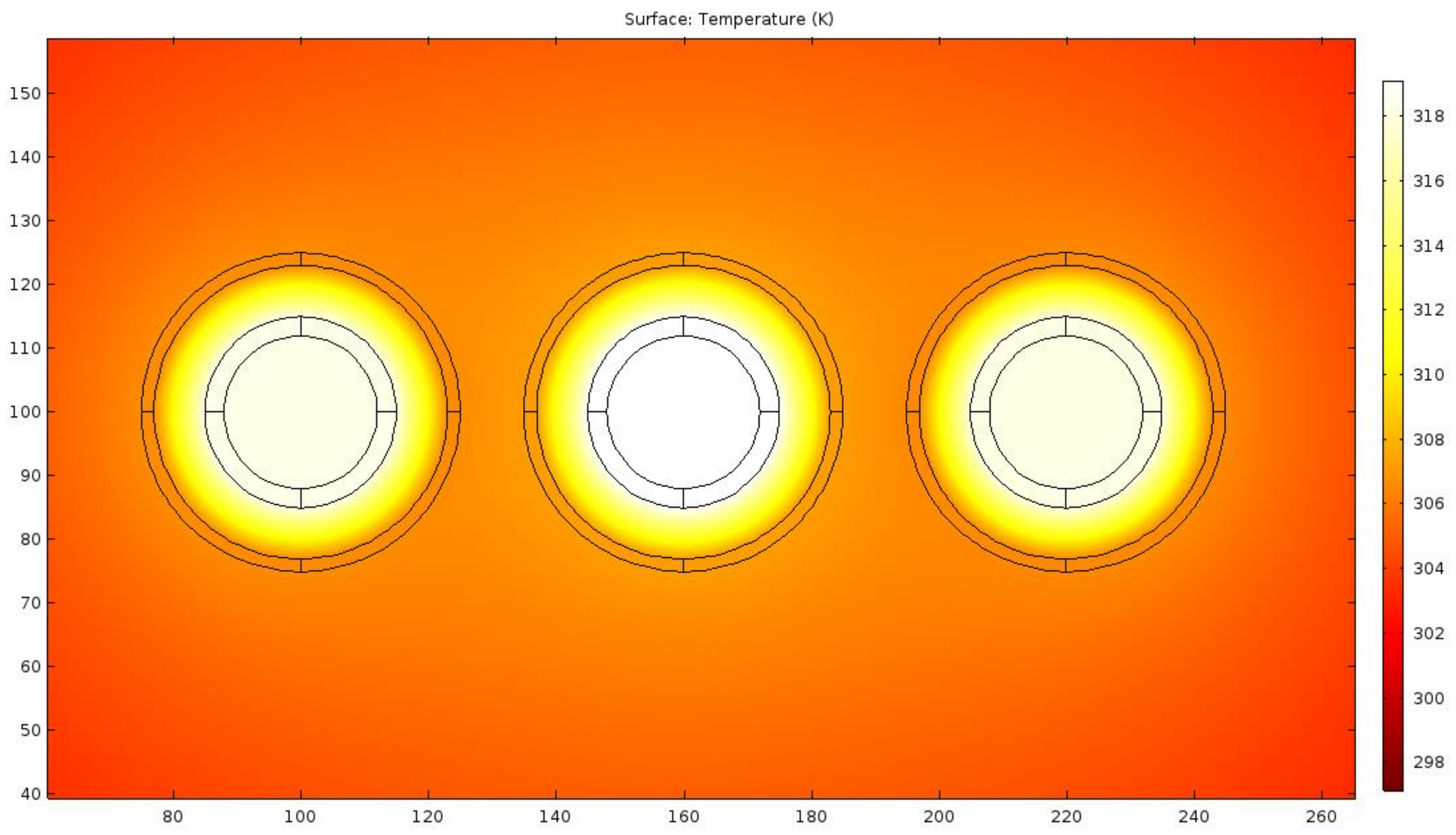
Apart from analytical calculation, computer simulations for high-current busduct system temperature were also performed with the aid of the commercial COMSOL software, using two-dimensional finite elements. The results of the computations are presented in Figure 6.

To carry out the simulation in the COMSOL software, the electromagnetic heating interface, using magnetic fields and heat transfer in solids modules, was used. The values of the material parameters, such as conductivity, magnetic permeability, etc., were taken from the material library available in the COMSOL software. For aluminum, they are γ = 33 MS·m⁻¹, ${\mu }_0=4\pi {10}^{-7}\frac{H}{m}$ and $\lambda =200\frac{W}{mK}$. The radiation was taken into account by setting the boundary condition, known as diffuse surface, on the edges of the areas and by introducing the emissivity coefficient on these surfaces (ε = 0.6). In turn, a natural convection was taken into account by applying the heat transfer in fluid condition to the areas of gas presence and setting the velocity field option at 0.01 m/s along the y axis. Physics-controlled mesh was used. Elements size was set as finer.

For a more accurate analysis, the temperature distributions in phases L1 and L2 (according to Figure 7), are presented in Figure 8 and Figure 9, respectively.

The experimental tests presented in this section confirmed the correctness of the analytical method of calculating temperature in high-current busducts. Differences between the temperature values calculated using the COMSOL software and the values obtained by the analytical method (Table 3) were due to the fact that the phase conductors in the analytical method were treated as filaments. The COMSOL software is based on the finite element method and, with the high density of the discretization mesh, the accuracy of the mapping phenomenon was greater. Differences between temperature values calculated with both methods revealed that, the greater the temperature, the smaller the distance between the particular phases.

4. Conclusions

This paper presented an analytical approach to the solution of the temperature in the three-phase high-current busduct. The proposed method allowed us to calculate temperature rise in a set of tubular busducts.

The analytical method was validated using the commercial COMSOL software and laboratory measurements. The mathematical model took into account the skin effect and proximity effects, as well as the electromagnetic coupling between phase conductors and enclosures. The results from the measurements indicated that the analytical method can be used to predict the temperature of any such tubular busduct system with good accuracy. The model predictions were found to be in very good agreement with the measurements.

Temperature distributions in high-current busducts are usually calculated using numerical methods. Numerical methods allow for the analysis of busduct temperature in various geometric systems, whereas analytical methods are dedicated to specific geometries of busducts. However, the use of numerical methods in the design and optimization processes made it very difficult to generalize the results and to derive simple dependencies supporting the design of specific types of busducts. In turn, the use of analytical methods to analyze specific systems required the use of many simplifying assumptions. Despite the use of some simplifying assumptions, the proposed analytical approach allowed the discovery of the general relationships between various parameters and temperatures. Each extension of an assumption (e.g., taking into account nonlinearities) significantly increased the difficulty of the analytical solution. Moreover, in thermal calculations, based on solving the Fourier-Kirchhoff equation, a significant difficulty is the calculation of convective and radiative heat transfer coefficients. The phenomenon of convection occurring in high-current busducts is related to the movement of a fluid, and, therefore, its description is not sufficient for the law of conservation of energy itself. However, it is also necessary to take into account the law of conservation of mass, momentum and, for gases, the equation of state. As a result, attempts to analytically calculate the value of the convective heat transfer coefficient for real systems led to extremely complex mathematical models. Therefore, in the problem of natural convection, the heat transfer coefficient is usually determined by semi-empirical methods resulting from the theory of similarity. However, regardless of the method used to determine the heat transfer coefficient, its significance in thermal calculations seems the highest. In further research, the proposed analytical method will be tested for more complicated GILs, e.g., three-pole busducts in an enclosure.