Response of a Tensegrity Simplex in Experimental Tests of a Modal Hammer at Different Self-Stress Levels

Abstract

The natural frequencies and eigenmodes of the tensegrity simplex are determined experimentally in impact hammer tests. To study an effect of prestressing, the tests are carried out on a physical model 1.2 m high and 0.5 m diameter with build-in transducers for measuring actual values of forces in cables at 13 prestress levels. The recorded data for each pre-stress level from three three-axial accelerometers are combined to extract the first five natural frequencies and modes by means of the method of experimental modal analysis. It was experimentally confirmed that the first rotational frequency depends on the pre-stress level and its sensitivity to the self-stress state is high enough to be successfully used in vibrational health monitoring. A proprietary formula was proposed for the relationship between frequency and the pre-stress level to control the dynamic properties of the simplex. An excellent comparison between the experimental results of the frequency and the formula was obtained. A comparison of numerical results of the finite element method with truss element and experiment is also shown.

1. Introduction

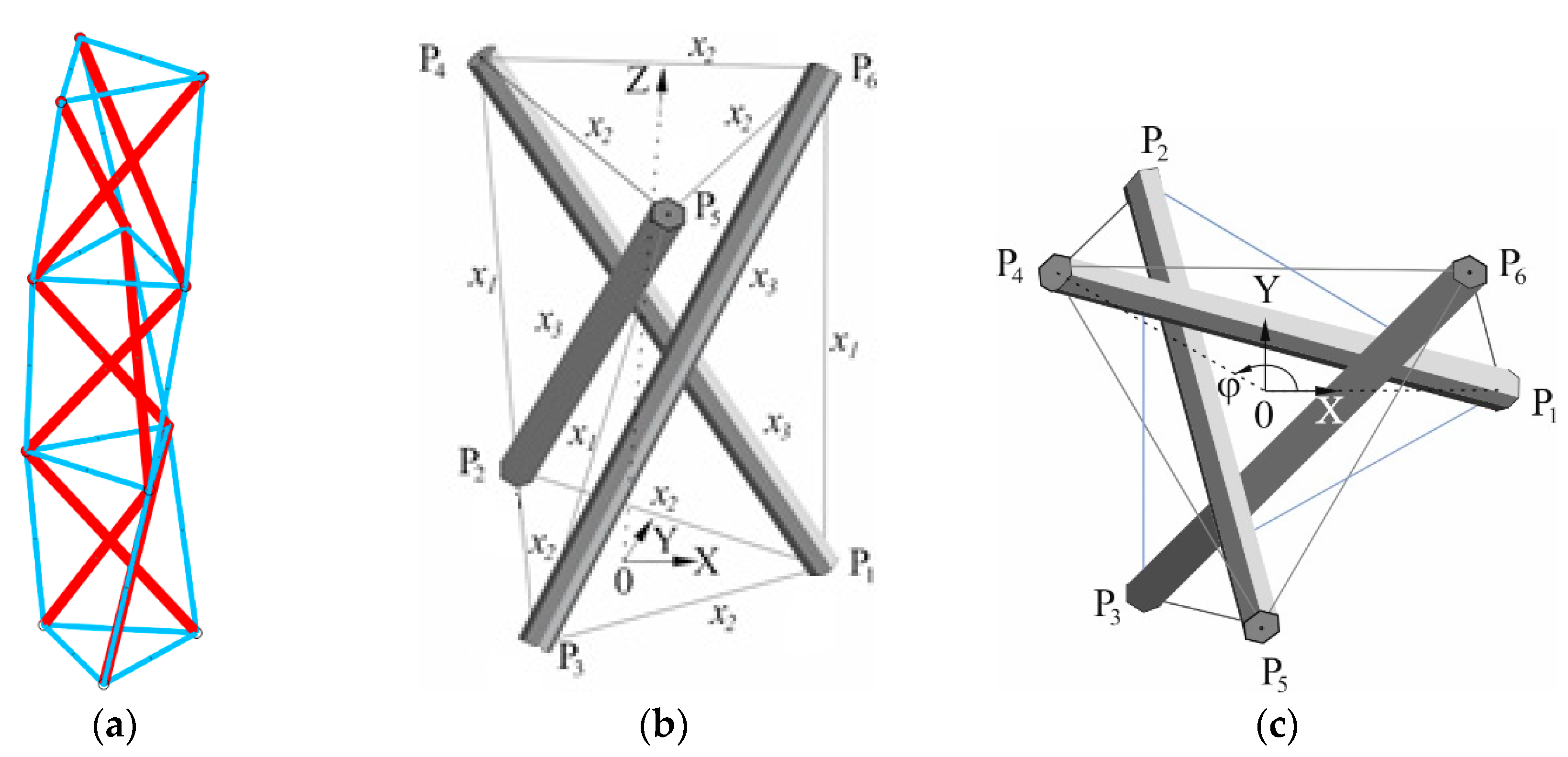
Tensegrity structures are built from compressed struts and tensioned cables. External loads can only be applied at the nodes, which connect elements using ball joints. The system stability and load-bearing capacity is obtained after inducing the prestressing force in its elements. Therefore, from the mechanical point of view, tensegrities can be regarded as a special class of spatial truss. A known example of these types of structure is a tensegrity column composed of several moduli, each of them being a tensegrity simplex (Figure 1). The tensegrity simplex as the fundamental three-dimensional module of low complexity is often called the regular minimal tensegrity prism [1]. It is constructed with three struts and nine cables. Six cables form two equilateral triangles which create horizontal bases of the module. The bases are interconnected between themselves by three other cables and three struts.

The history of tensegrity structures starts from the year 1921 when a sculpture of Karl Ioganson was presented at an exhibition in Moscow [2]. Better known in the west is the artist Kenneth Snelson, creator of his X-Piece structure from 1948 [3,4]. Following the pattern of sculptures by Snelson, the architect Richard Buckminster Fuller patented a class of cable-bar assemblages in 1961, which he named tensegrity structures as an abbreviation of tensile integrity [5].

Although elements forming tensegrity structures can deform in the range of small strains, the structure as a whole can experience large displacements. Therefore, their analysis needs to take into account geometrical non-linearity, where the equilibrium path is a function of the pre-stress level. The response of the Simplex to uniaxial compression was studied numerically in [6] and, further, experimentally in [7]. Both surveys have proven that the module may experience softening or stiffening type of response, as well as that it is a dependent on geometry, prestress level and stiffness of the members. Simplex module design examples, built from highly-elastic polyamide ropes and taking into account geometric nonlinearity, were shown in [8,9] with an incremental-iterative script written in Matlab programming language. Despite the non-linear approach, after inducing the prestress to the structure at a designed magnitude, the computational task can often be linearized, as in many simulation approaches. After the prestressing, small vibrations around the equilibrium points may be analyzed i.e., modal analysis can be used with linearization of these vibrations. This kind of a preliminary research of the simplex with innovative cables was presented in [10]. Determined natural frequencies and modes can further be used to calibrate or validate numerical solutions. In tensegrity structures, the function of the first natural frequency vs. the magnitude of prestress is utilized in vibrational health monitoring or active stiffness control using servomechanisms.

In 1986 Rene Motro conducted a study [11] on a tensegrity simplex, in terms of static and dynamic analysis. The equilibrium path of the axially loaded module, as well as six natural frequencies, were determined. The module was, however, not prestressed. In [12] the relation between the pre-stress and natural frequencies was studied numerically for two-dimensional tensegrity trusses. The results stated that the change of pre-stress level causes the natural frequencies to either rise or fall. The effect of the self-stress on the dynamic properties of the basic spatial tensegrity modules was analyzed in the papers [13,14,15,16]. A dynamic model of the simplex as a system of single-degree-of-freedom subjected to rotation about its vertical axis was discussed in [17]. An active controlled tensegrity was analyzed dynamically in [18], which was a part of a Tensarch project [19]. A solution to attenuate the first natural frequency in order to diminish the response of the analyzed structure was proposed. A five-module tensegrity was studied experimentally and numerically in [20] by means of vibrational behavior, taking into account the effect of active strut movement. The pre-stress effect on the response of the tensegrity structures was also numerically studied, recently in [21] and in [22], with an emphasis on a road bridge appliance. Numerical analyses of statically and dynamically loaded structures was also analyzed in [23]. The effect of the self-stressing force on self-diagnosis, self-repair and active control of a tensegrity structures and modules were analyzed numerically in [24], where it was proven that it is possible to compensate potential damage of the structure by adjusting the prestress level.

The vast majority of presented surveys were of the numerical type, and there were no experimental validations of obtained results. On the other hand, Motro’s experimental analysis did not consider different prestress levels, while the Tensarch project investigations were performed on the different tensegrity grid and were focused on the structural control. Therefore, this study aims to fill the literature gap in terms of experimental identification of modal parameters, taking into account the prestress level of the tensegrity simplex and the contemporary method of measurement.

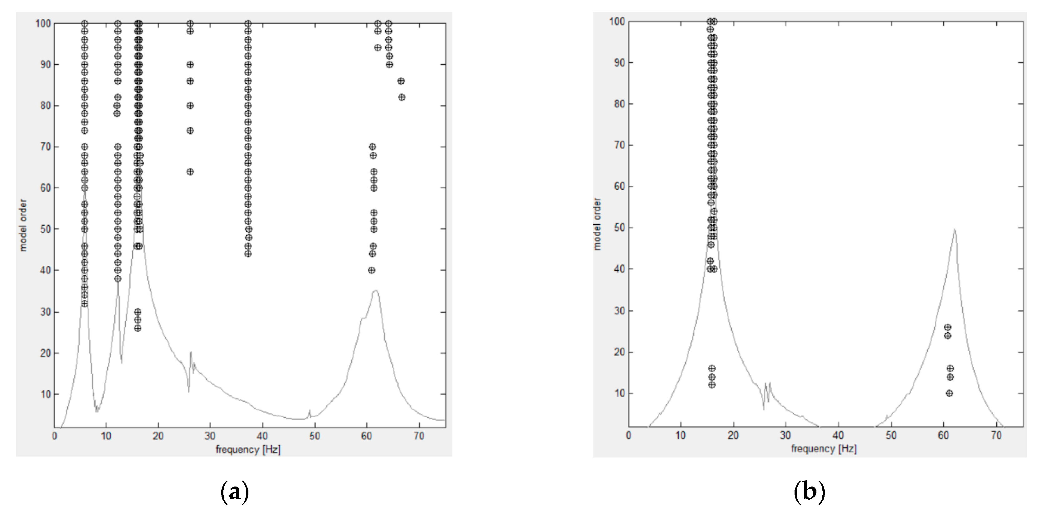
The utilized method is the experimental modal analysis. The method is used in many areas, e.g., for dissipation estimation in materials [25], and for fatigue assessment of tools [26]. However, a majority of tests are considered with structural behavior i.e., determining the damping ratios, natural frequencies and corresponding modes—see, e.g., [27]. In this study, recorded data from an impact hammer strike were post-processed with a system identification method and further extracted using a Matlab [28] toolbox [29].

The article is written in the following order: Section 2 presents the self-stress states of the analyzed module and the description of the physical model, Section 3 includes the process of the experimental modal analysis with its results and the Section 4 includes a discussion with conclusions.

2. The Prestressability of the Experimental Model and Vibration Measurements

Symmetrical prestressable configurations of the left-handed tensegrity simplex are considered. The symmetrical configuration is commonly used in theoretical models of the simplex and it can be described by three variables, e.g.,: the radius $r$ or the side length $L=r\sqrt{3}$ of the triangles, the height $h$ denoting the distance between the horizontal triangles, and the twist angle $\phi$ between the projection of the line $\mathrm{0–4}$ onto the horizontal plane and the $X$-axis (Figure 1). The stable equilibrium configuration is for the angle $\phi =5\pi /6$ and it is taken as the reference configuration. In the Cartesian coordinate system $(0\mathrm{XYZ})$, with the origin at the center of the bottom triangle, we can identify coordinates of the nodes $P_i(\begin{array}{ccc}{X}_i& Y_i& Z_i)\end{array}\hspace{1em}i=1,\dots ,6$ as:

$$\begin{array}{l}{P}_1(\begin{array}{ccc}r& 0& 0\end{array}),\hspace{0.17em}{P}_2(-\begin{array}{ccc}r/2& r\sqrt{3}/2& 0\end{array}),\hspace{0.17em}{P}_3(-\begin{array}{ccc}r/2& -r\sqrt{3}/2& 0\end{array}),\hspace{0.17em}{P}_4(\begin{array}{ccc}r\cos \phi & r\sin \phi & h)\end{array},\\ P_5[\begin{array}{ccc}r\cos (\phi +2\pi /3)& r\sin (\phi +2\pi /3)& h]\end{array},\hspace{1em}{P}_6[\begin{array}{ccc}r\cos (\phi +4\pi /3)& r\sin (\phi +4\pi /3)& h\end{array}],\end{array}$$

(1)

from which additional geometrical parameters can be calculated, e.g., the lengths s and b of the cross-cables and the bars, respectively:

$$s=r\sqrt{{\left(h/r\right)}^2+2+\cos \phi -\sqrt{3}\sin \phi },\hspace{1em}b=r\sqrt{{\left(h/r\right)}^2+2\left(1-\cos \phi \right)}.$$

(2)

The tensegrity simplex is characterized by the one self-stress state that ensures its stability by activating the geometrical stiffness. The self-stress state introduced initially in the members before applying loads has a direct impact on the structural response depending on its level. Together with the cross-sectional areas of tensioned and compressed members, the initial self-stresses are the design parameters that affect the structural performance and cost of a tensegrity structure. The self-stress level $p_0$, which describes the general self-stress state in the tensegrity simplex can be defined as a normal elongation of the cross-cables, i.e., as the strain:

$$p_0=(s_0-s_N)/s_N,\hspace{1em}{s}_N=r\sqrt{{\left(h/r\right)}^2+2-\sqrt{3}},$$

(3)

where the cross-cable length $s_N$ is calculated based on the formula (2) for the angle $\phi =5\pi /6$ at which the tensegrity equilibrium occurs. It follows from (3) that after pre-stressing at a level $p_0$, the length of the cross-cables is equal to $s_0=s_N(1+p_0)$. The other lengths, i.e., the length of the base triangles $L_0$ and the length of the bar $b_0$ can be computed from the analytical model—see [6,8] as:

$$L_0=\frac{E_L{A}_L(1+p_0)L_N{s}_N}{p_0(E_L{A}_L{s}_N-\sqrt{3}{E}_s{A}_s{L}_N/3)+E_L{A}_L{s}_N},\hspace{0.17em}{b}_0=s_N(1+p_0)\hspace{0.17em}\hspace{0.17em}\sqrt{1+\frac{6\sqrt{3}\hspace{0.17em}{E}_L^2{A}_L^2{L}_N^2}{{\left[p_0(3E_L{A}_L{s}_N-\sqrt{3}{E}_s{A}_s{L}_N)+3E_L{A}_L{s}_N\right]}^2}}$$

(4)

where $E_s,\hspace{0.17em}{E}_L$ are the Young’s moduli and $A_s,\hspace{0.17em}{A}_L$ are the cross-section areas of the cross and horizontal cables, respectively. When using the finite element method, we can obtain these lengths by iterative procedures, while having a physical model, by measurements.

Figure 1 shows, that it is possible to calculate the self-stress state of module, without external loading and without any supports in terms of an arbitrary chosen force density $t$ i.e., the ratio between the member force and the member length as $t_{16}=t_{24}=t_{35}=t$ in the cross-cables, $t_{14}=t_{25}=t_{36}=-t$ in the bars and $t_{12}=t_{13}=t_{23}=t_{45}=t_{46}=t_{56}=t/\sqrt{3}$ in the horizontal cables, because for the tensegrity simplex in the equilibrium configuration $\phi =5\pi /6$ without any external loads, the following relationship can be written:

$$\left\{\begin{array}{c}{x}_1\\ x_2\end{array}\right\}=-x_3\left\{\begin{array}{c}1\\ \frac{1}{\sqrt{3}}\end{array}\right\}$$

(5)

where the force density $x_3<0$, i.e., it is assumed to be negative if the bars are under compression.

After the prestressing, the normal forces in the cross-cables $N_s^{}$, the horizontal cables $N_L^{}$ and the bars $N_b^{}$ are:

$$N_s^{}=x_1{s}_0=E_s{A}_s{p}_0,\hspace{1em}{N}_L^{}=x_2^{}{L}_0=\frac{1}{\sqrt{3}}{x}_1^{}{L}_0=\frac{L_0}{\sqrt{3}}\frac{E_s{A}_s}{s_N}\frac{p_0}{1+p_0},\hspace{1em}{N}_b^{}=x_3^{}{b}_0=-x_1^{}{b}_0=-\frac{E_s{A}_s{p}_0}{s_N(1+p_0)}{b}_0,$$

(6)

where $x_1$, $x_2$ and $x_3$ and denote the force densities acting in the cross-cables, horizontal cables and bars, respectively.

Taking in the formulas (6) $p_0=N_s/E_s{A}_s$, the self-stress state can be also expressed in terms of the force in the cross-cables as the parameter $S=N_s$. It is worth mentioning, that the unknown three force densities need to be known, when the deformation of the module preserves the parallelism of the two base triangles, e.g., when the module is under uniform and axial loading.

The coordinates, element numerations, and lengths of the simplex used in the survey are presented in

Table 1. Data on the tested simplex module ($\phi =5\pi /6$).

Self-Stress State
$t_{14}$ (bars)			$t_{12}$ (horizontal cables)					$t_{16}$ (cross-cables)
−t			$t/\sqrt{3}$					t
$L_{14}=b$ [m]			$L_{12}=r\sqrt{3}$ [m]					$L_{16}=s$ [m]
1.280 1			0.431 1					1.193 2
Node	Coordinates 3 [m]				Node and member numbers
	X	Y		Z
$P_1$	0.249	0		0	horizontal cables					cross-cables
$P_2$	−0.125	0.216		0	1	$P_1-P_2$	7		$P_4-P_5$	4	$P_1-P_6$
$P_3$	−0.125	−0.216		0	2	$P_2-P_3$	8		$P_5-P_6$	5	$P_2-P_4$
$P_4$	−0.216	0.125		1.186	3	$P_1-P_3$	9		$P_4-P_6$	6	$P_3-P_5$
$P_5$	0	−0.249		1.186	Bars
$P_6$	0.216	0.125		1.186	10	$P_1-P_4$	11		$P_2-P_5$	12	$P_3-P_6$

¹ In situ measurement, ² Calculated from (2) for $h=r\sqrt{{\left(b/r\right)}^2-2-\sqrt{3}}=1.186m$, ³ Calculated from (1).

, as well as, the self-stress state according to the symmetrical theoretical model.

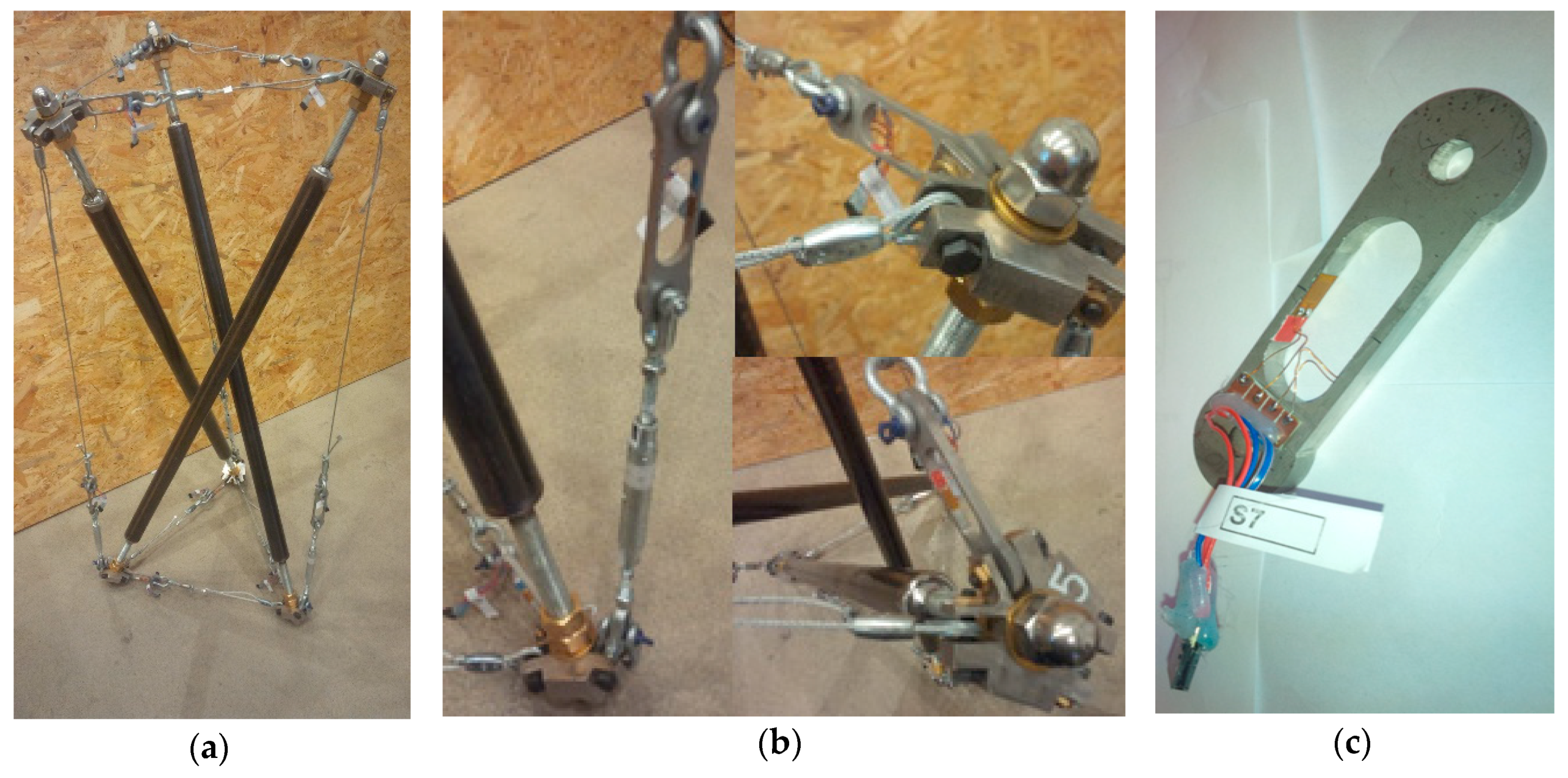
The experiments were performed on the full-scale physical module. The view of the model and some technical details are presented in Figure 2. The bars made of a steel S355 were built from rods of the circular hollow section 42.4 × 2 mm, in which M20 bars were welded into edge parts. The linear density of the bars, i.e., the masses per length of both used sections are similar. The bearing capacity of the bars under compression is sufficient high to withstand expected in experiments the pre-stress levels. The cross and horizontal cables were created using a 3 mm nominal diameter steel line made of 19 wires and thimbled on each side. The net area of the cross-sections of the line is given in

Table 2. Material parameters of the simplex.

	Bars	Horizontal Cables	Cross-Cables
Young’s modulus [GPa]	210	56.0 1	81.1 1
Cross section [mm2]	253.8	5.25	5.25
Mass per length [kg/m]	1.990	0.0436/0.516 2	0.0436/0.516 2
Single joint mass [kg]	0.897	Total model mass [kg]	16.205

¹ Values obtained in the experiment, ² Non-physical, reduced value taken into finite element method (FEM) consistent mass matrix calculations.

, where materials, cross sections and masses of the physical model are gathered. The equivalent moduli of elasticity are presented in Table 2 for the cross and horizontal cables, since they are made apart from steel lines, also of force transducers, roman screws and shackles. The moduli were established based on experimental uniaxial tension tests.

The minimal failure force, given by the manufacturer, is equal to 7.26 kN. The design value of 6.30 kN can be assumed as the bearing capacity after taking a partial material factor. Each cable had attached a force sensor (Figure 2c), while three cross-cables had also additionally attached a roman screw in order to implement and control the prestress level. Nodes were laser cut out of a 20 mm thick stainless steel sheet and further countersigned for M8 bolts, which held the cables. A connection of the bars and nodes was created by regulation of two steel nuts, while a connection of cables and nodes was created using M8 screws (Figure 2b). Crafted specially for the model, the force sensors were attached to all nine cables (Figure 2c). The mass of a single joint was 0.897 kg. They were designed to work with electro-resistive strain gauges, where two active arms are placed on the opposite sides of the four-arm bridge (so called Wheatstone half bridge configuration). The body of the sensor was precisely water cut out of 6 mm thick stainless steel sheet and further processed to obtain a clear surface. The strain gauges were mounted on the two inner sides of the body, with special attention to manufacturers’ requirements [30]. The finisher force sensors were also calibrated for the force using the strain gauge bridge and a universal testing machine to obtain the force-strain function and for the temperature using the strain gauge bridge and climate chamber to obtain the temperature-strain function. This enabled proper readouts on the force during the tests to be obtained, where also temperature variations were taken into account.

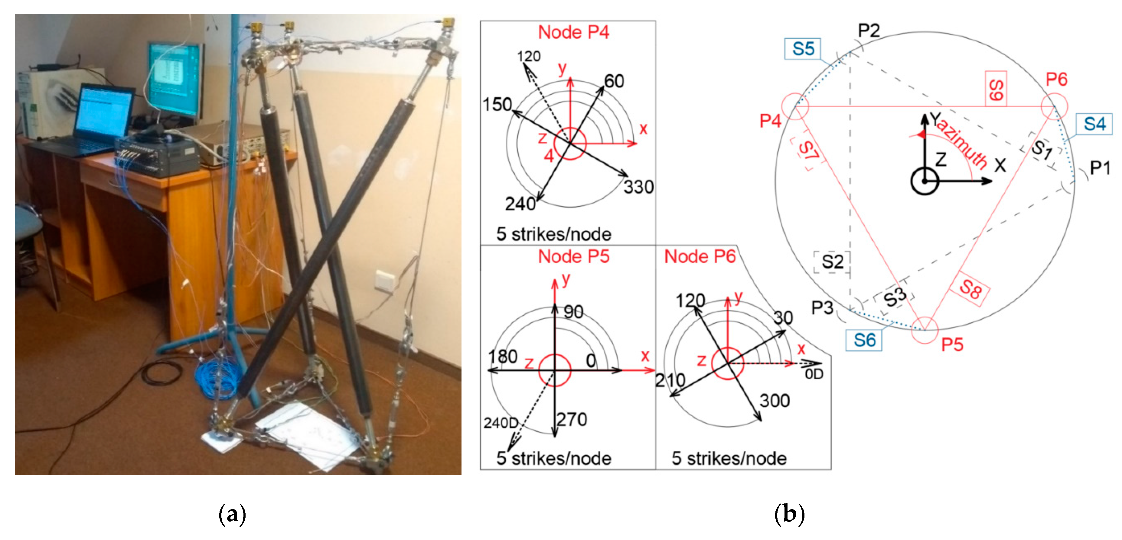
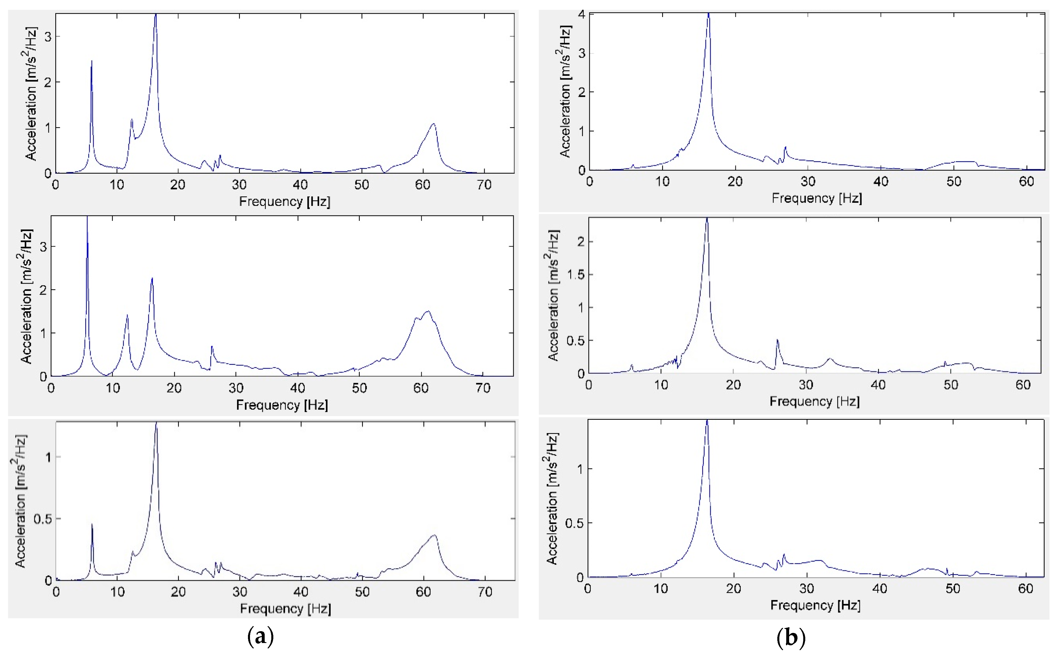
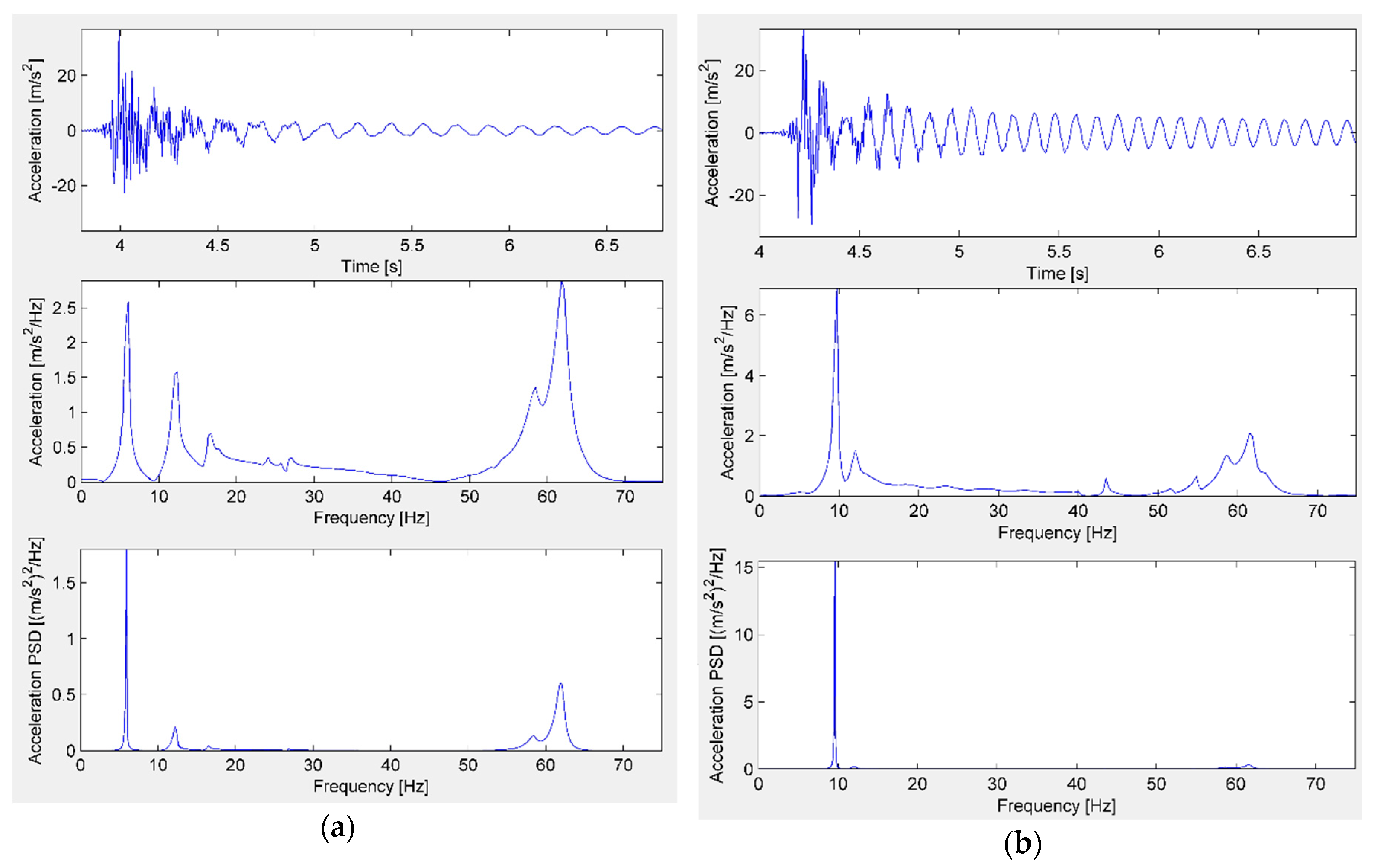
The testing standpoint was composed of the simplex module with three attached, triaxial piezoelectric accelerometers on top of its three nodes, a strain gauge bridge with the force sensors, a dynamic analyzer and impulse hammer (Figure 3). The strain gauge bridge was used to control the values of forces in nine cables—three cross-cables and six horizontal cables in the top and bottom triangle. The dynamic recorder was used to record the values of applied impulses induced by the modal hammer and accelerations of the three, tri-axial accelerometers attached to the upper nodes of the simplex.

The methodology of the test was based on the method of the experimental modal analysis, where both types of signal—the force and accelerations are recorded in the time domain—from the modal hammer impulse and from the accelerometers in the upper nodes. The method utilizes all signals recorded in the test, i.e., all forces that are applied to the structure are measured. Ambient forces such as wind or traffic can be excluded. This method is based on obtaining both the impulse signal and the acceleration signal. At the excitation, piezoelectric transducers change the mechanical vibration energy into an analogous electrical signal, which is afterwards amplified by the amplifier. Furthermore, the analyzer digitizes the analogous signal into discrete series. The time resolution (number of samples measured in time) is dependent on the sampling rate, while the resolution of the recorded magnitudes is dependent on the bit depth.

A complete measuring system is usually composed of three elements: an excitation mechanism, a power amplifier, an analyzer and at least one transducer.

The study was performed using a data acquisition and recording system TEAC brand, model LX-110, using the dedicated software [31]. The acceleration transducers are of the typical, triaxial type consisting of a seismic mass and piezoelectric crystals enclosed in one body. Their parameters are listed in [32]. The hammer is built of a handle connected with a striking head. The idea is similar to the accelerometers, yet providing data on the force values. A detachable mass, as well as, a set of hammer tips with different stiffness enables to adjust the induced frequency of the structure. Generally, the heavier the hammer and softer the tip, the lower the frequencies that are induced. Data on hammer utilized in the test are available in [33].

Figure 3b presents the experimental global coordinate system, where it was possible to measure accelerations of nine signals 4x, 4y, 4z, 5x, 5y, 5z, 6x, 6y, 6z in the one strike of the impulse hammer, as a source of excitation, together with this one force signal induced by this hammer at each pre-stress level. The directions of the strikes are shown also in Figure 3b. One hundred and thirty five acceleration signals and 15 force signals were recorded for each prestress level. The 13 different prestress levels were applied on the whole as shown in

Table 3. Member forces for the each prestress level.

Level		Cables [N]			Bars 2 [N]	Level		Cables [N]			Bars 2 [N]
No	${\mathit{p}}_0\left[{10}^{-6}\right]$	Cross 1	Base 1	Base 2		No	${\mathit{p}}_0\left[{10}^{-6}\right]$	Cross 1	Base 1	Base 2
1	618	263 ± 27	75 ± 13	55	−282	8	5082	2164 ± 28	646 ± 20	450	−2322
2	1294	551 ± 37	169 ± 17	115	−591	9	6135	2612 ± 35	766 ± 23	542	−2802
3	2104	896 ± 40	263 ± 16	187	−961	10	6877	2928 ± 42	849 ± 24	607	−3141
4	2741	1167 ± 38	345 ± 18	243	−1252	11	7264	3093 ± 43	892 ± 23	641	−3318
5	3368	1434 ± 35	421 ± 18	298	−1538	12	7788	3316 ± 45	957 ± 25	687	−3558
6	3981	1695 ± 31	500 ± 20	352	−1818	13	8418	3584 ± 40	1025 ± 25	742	−3845
7	4413	1879 ± 29	559 ± 19	391	−2016

¹ Experimental values, ² Calculated from (5).

in terms of the measured forces in the cross and horizontal (base) cables.

A distribution of the member forces between elements of the same type, i.e., the lower horizontal cables (1–3), the upper horizontal cables (7–9) and the cross-cables (4–6) for exemplary 4th and 13th prestress levels are presented in Figure 4 and correspond with numeration in Table 1. The forces are closely related with each other among each of the three groups during the prestressing process. The theoretical distribution of the member forces seems to be preserved with typical experimental fluctuations connected with crafting and measuring accuracy of the physical model.

3. Results

The presentation of the obtained results are divided into two subsection, from which the second part of the experimental study on our own physical model is of great interest. The modal parameters of the tensegrity simplex, which were determined utilizing the toolbox [29], are presented and discussed in this part together with recorded data as obtained in impact hammer tests.

3.1. Numerical Analysis on Small Vibrations

As mentioned before, a linearization of vibrations around the equilibrium state was assumed. For a chosen pre-stress level, these vibrations are determined in numerical analysis using equations of motion as for a linear multi-degree-of-freedom system of the structure, i.e., by the system of ordinary differential equations governing vectors of order $n$ of the displacements $u(t)$ due to applied dynamic forces $p(t)$ in the matrix equation:

$$M\ddot{u}(t)+C\dot{u}(t)+K_{T}u(t)=p(t)$$

(7)

where $n$ is the number of independent degrees-of-freedom (DOF), the square matrices of order $n$$M,\hspace{0.17em}C,\hspace{0.17em}{K}_T$ are the mass, damping and tangent stiffness matrices and $\ddot{u},\hspace{0.17em}\dot{u}$ are the resulting acceleration and velocity vectors. The complete solution $u(t)$ consists of two contributions: the initial part of the response induced by the initial conditions and the particular solution which satisfied the forcing function $p(t)$. When $p(t)=0$, a very frequently occurring problem in structural dynamics is the free vibration equation to be solved, usually by means of the finite element method as a linearized eigenproblem:

$$K_T{\phi }_k-{\omega }_k^{2}M{\phi }_k=0,$$

(8)

The solution lies in the spectral decomposition of the matrix $M^{-1}{K}_T$. It gives the natural modes and frequencies of the analyzed structure. If the analyzed equlibrium state possess (n) DOFs, then the spectral decomposition of (8) provides (n) frequencies ${\omega }_k$$({\omega }_1<{\omega }_2\dots <{\omega }_n)$ and (n) corresponding eigenvectors ${\phi }_k$.

According to the finite element method (FEM), the system matrices $K_T$ and $M$ are typically build from the element matrices $k_T$ and $m$, which are determined in the local coordinate system. The geometric stiffness element matrix $k_G(S)$ dependent on the pre-stress level, and the elastic stiffnes element matrix $k_E$, build the tangent element matrix $k_T$ by simple addition. The element matrices for the two-node straight finite element for the spatial truss are:

$$\begin{array}{l}{k}_T=k_E+k_G\hspace{1em}\hspace{1em}\hspace{0.17em}\hspace{0.17em}\hspace{0.17em}{k}_E=\frac{E{A}_0}{l_0}\left[\begin{array}{cc}\hspace{0.17em}\hspace{0.17em}{I}_0& -I_0\\ -I_0& \hspace{0.17em}\hspace{0.17em}{I}_0\end{array}\right]\hspace{1em}\hspace{0.17em}\hspace{1em}{k}_G=\frac{S}{l_0}\left[\begin{array}{cc}\hspace{0.17em}\hspace{0.17em}\hspace{0.17em}I& -I\\ -I& \hspace{0.17em}\hspace{0.17em}I\end{array}\right]\\ m=\frac{\rho A_0{l}_0}{6}\left[\begin{array}{cc}2I& I\\ I& 2I\end{array}\right]+\left[\begin{array}{cc}{m}_1^{}I& I\\ I& m_2^{}I\end{array}\right]\hspace{0.17em}\hspace{0.17em}I=\left[\begin{array}{ccc}1& 0& 0\\ 0& 1& 0\\ 0& 0& 1\end{array}\right]\hspace{0.17em}\hspace{0.17em}{I}_0=\left[\begin{array}{ccc}1& 0& 0\\ 0& 0& 0\\ 0& 0& 0\end{array}\right]\end{array}$$

(9)

where $S$ is the element force according to the self-stress and $m_i$ are masses of the nodes.

Some results of a numerical analysis of small vibration conducted by means of our own finite element program are shown in Section 4. The coordinates as well as element lengths and numbering used in the FE analysis are presented in Table 1 (each member is a single finite 3D truss element). The Young’s moduli, cross section and mass per length of the elements were taken as shown in Table 2. Calculations for two types of mass matrices were undertaken: a lumped-mass idealization with the diagonal terms and for the consistent-mass formulation basing on the effective mass of the cables calculated using the weight of the experimental model. The prestressing forces in cross-cables were equal to the measured forces in these elements for each prestress level taken from Table 3. Prestress forces in struts and horizontal cables were distributed using member lengths and the self-stress vector from Equation (5) (based on the known forces in cross-cables). The numerical analysis of the tensegrity simplex was performed for two types of boundary conditions: as a system of the nine dynamic DOFs—three for every upper base traingle node with the bottom triangle fixed the floor, and as a system of 12 DOFs with the bottom supports preventing six DOFs. In general, the boundary conditions may have a great effect on the results of the numerical calculations. However, for the first natural mode, the difference is negligible since the mode is rotational around the vertical axis. The difference may be more visible for modes of a flexible type.

3.2. Processing the Signals and Modal Parameters

From the three known dynamic vibration tests, i.e., forced, ambient and combined, the first was used with an excitaion induced by the impact hammer.

In general, the well-known experimental modal analysis consists of: (1) recording of the signals, (2) identification of the system and (3) approximation of the modal parameters. The last step can be performed by free vibration analysing of the identified system model from step (2), i.e., by modal decomposition. The model is a mathematical solution, estimated on a basis of measured data and can be of parametric or non-parametric type. The latter can be described in a tablularized form, as for example, the frequency response functions (FRF).

Using the Laplace transform of (7) and neglecting the initial conditions provides the frequency-domain method for analysis of response of linear systems to excitations varying arbitrarily with time in the matrix equation:

$$Z(s)U(s)=P(s),$$

(10)

with the dynamic stiffness $Z(s)=M\hspace{0.17em}{s}^2+C\hspace{0.17em}s+K_T$ and $s=i\omega ,\hspace{0.17em}\hspace{0.17em}i=\sqrt{-1}$. Inverting above equation yields:

$$U(s)=H(s)P(s),$$

(11)

with the transfer function matrix $H(s)=Z^{-1}(s)$. The frequency-domain method is an alternative approach to the time-domain method and provides an efficient means of a predicting response. The frequency response analysis can be particularly useful if the linear response of a system subjected to a continuous series of harmonic excitations, i.e., to the periodic forcing function with a frequency $\omega$ is sought. Steady-state response is then given as a frequency sweep through a specified range of frequencies. The response for each excitation frequency ω can be determined from (11). The ‘response function’ $H(\omega )$ is the Fourier transformation of the response matrix.

Each element of the matrix $H(\omega )$ can be itself a frequency response function (FRF) and it is most likely to be able to measure in practice. From FRFs it is possible to determine modal characteristics of structure, which are amenable to direct measurement. However, the measured frequency response functions ought to be subjected to a range of curve-fitting procedures in an attempt to find the mathematical model, which provides the closest description of actually observed behavior. According to the modal theory of mechanical systems, the FRF matrix can be decomposed as:

$$H(\omega )={\displaystyle \sum _{r=1}^N\left(\frac{{\varphi }_r^{}{L}_r^T}{i\omega -{\lambda }_r^{}}+\frac{{\varphi }_r^{*}{L}_r^H}{i\omega -{\lambda }_r^{*}}\right)},$$

(12)

with such modal parameters as the poles ${\lambda }_r={\sigma }_r+i{\omega }_r$, vectors of the mode $r$, the mode shape ${\varphi }_r$ and modal participation factors $L_r$. One element ${\lambda }_r$ contains both the natural frequencies $f_r$ and damping ratios $d_r$ for the $r\mathrm{th}$ normal mode of vibration. They can be determined as $f_r={\omega }_r/(2\pi )$, $d_r=-{\sigma }_r/\sqrt{{\sigma }_r^2+{\omega }_r^2}$, where the number of modes may differ from the number of measured output degrees of freedom and the number of input forces. The meanings of symbols used in (12) are: ${(.)}^{\ast }$—a complex conjugate, ${(.)}^T$—a transpose of the matrix, ${(.)}^H$—a complex conjugate transpose of the matrix (a Hermitian transpose).

To identify modal characteristics of the simplex three steps have been chosen: (1) the hammer test, (2) the method pLSCE and (3) a stabilisation diagram with peak picking. All steps of the experimental modal analysis (EMA) were performed using the Macec toolbox [29], using the deterministic poly-reference least squares complex frequency domain method (pLSCF).

The natural frequencies identified are gathered in

Table 4. First five natural frequencies for 13 prestress levels.

	Frequency [Hz] of Mode No:						Frequency [Hz] of Mode No:
no	1 r	2 f	3 f	4 f	5 r	no	1 r	2 f	3 f	4 f	5 r
1	3.36	11.3	15.8	-	-	8	7.57	11.6	16.1	57.7	62.2
2	4.32	12.1	15.5	-	-	9	8.2	11.5	15.9	57.6	62.7
3	5.29	11.9	15.8	58.4	-	10	8.7	11.6	15.8	57.8	-
4	5.87	12.0	16.3	58.4	-	11	8.98	11.9	16.3	58.5	62.8
5	6.4	12.1	16.4	58.5	62.5	12	9.19	12.0	15.9	58.2	62.8
6	6.78	11.4	15.6	58.0	-	13	9.54	11.7	16.3	-	63.2
7	7.12	11.6	16.0	58.3	62.5

^r Mode of rotational type and ^f flexural type.

, while natural modes are presented in Figure 5. The modal parameters are obtained by connecting the results of modal testing through all setups. Two types of vibration were identified, a so called rotational and flexural mode. By rotational vibrations we will denote rotations of the upper horizontal triangle around the vertical z axis, i.e., three upper nodes are moving along the circle inscribed in the equilateral triangle of these upper nodes (Figure 5a). By flexural vibrations we will denote the rotations of the upper base triangles around the horizontal y axis (Figure 5b).

The signals were recorded with a relatively high, for the test purposes, sampling frequency of 1500 Hz. The acceleration signals did not need such high frequency, yet to record the detail of the short-time transient inducing signal generated by the impact hammer such a frequency was entered. The signals lasted nearly 16 s. The post-processing of the recorded signals involved clearing the offset and decimation by 10, which caused, due to the Nyquyst frequency and aliasing phenomena, the maximum value of frequency being equal to 75 Hz.

Figure 6 presents as an example the signals from the 4th node accelerometer after the FFT for directions x (upper), y (central) and z (lower) after the strike at azimuth 120 degrees (left) and 330 degrees (right). Comparing two different strike azimuths, it is seen that different vibration frequencies were induced. The strike of the direction perpendicular to the circle of the upper triangle at 330 degrees is inducing the dominant, well visible, single flexural mode of vibrations at approximately 16 Hz. This very strong visible frequency is presenting the mode, or as it is shown in stability diagrams, two very closely situated modes. The strike at 120 degrees induces the rotational and flexural modes of vibrations and can be used to find all modes. For this strike all directions of vibrations are showing the same frequencies, although with the different intensity. The frequencies are most clearly seen and they are of the flexural mode at approximately 16 Hz and less than those for the two rotational modes at approximately 5 and 62 Hz. Nevertheless, only the 4y acceleration signal (in the middle of Figure 6) shows clearly that the modes near 16 Hz are actually two different ones. This is not clearly visible when looking only on the signals 4x and 4z. Therefore, measuring three orthogonal directions is helping to find all modes that reveal themselves with different intensity.

Figure 7 presents the acceleration signals in time domain (upper), in the frequency domain (middle) and the power spectrum density of the acceleration in the frequency domain (lower) for the 4th (left) and 13th (right) prestress level. The comparison of the two presented signals shows, that the first natural frequency has increased significantly after the increase of the pre-stress level. For the 4th pre-stress level the concentration of natural frequencies gathers around the value of 6, 12 and 16 [Hz]. At the 13th pre-stress level, the modes are clearer and sharper, and the dominant frequency is induced around the value of 10 [Hz]. The diagram of the PSD acceleration presents an increase of the first mode, which is visible with the increase of the prestress level, where a change from approximately 6 to 10 Hz has occurred.

After the preparation of signals, the post-processing procedure was performed in order to extract natural modes and frequencies. The pLSCF method was used with the following parameters: frequency 1%, damping 5%, vector 1%, transfer norm 50%, the minimum modal phase collinearity 95% and minimum two identified natural modes in one setup. The explanation of the identification parameters and procedures can be found in e.g., [34].

Although choosing the frequency and modes from the stabilization diagram is somehow arbitrary, as shown in an exemplary way in Figure 8, this issue is especially important for tensegrity structures, where the resonance spectrum often includes very closely situated frequencies. This is the case for frequencies around 16 Hz in Figure 8, which is a result of a high degree of a structure’s symmetry. Therefore, third flexural mode (Table 4) had very closely related double eigenmodes. These double natural modes are both presenting a flexural mode for different directions of vibrations. Hence, interferring natural frequencies can be an obstacle in recognizing the correct resonance and is susceptible to human error. The natural frequencies and modes are better or worse seen in the stabilization diagrams, which are subjected to the direction of the measured and induced signal (Figure 8). To find a certain type of mode, it is good to induce only this mode. Figure 8b presents finding only two modes, both of the rotational type, after inducing the impulse for the tangential direction. To find all modes of the structure, it may be good to induce generally more of them by applying a randomly directed signal, such as presented in Figure 8a in the direction of 120 degrees for node P4, wherein one can see at least five modes of the rotational and flexural type.

4. Discussion

The first frequency depends on the self-stress state. This is due the fact that in the simplex one infinitesimal mechanism can be identified. The phenomenon is known in the literature. In the absence of prestressing, the first natural frequency should be zero, and after introducing the self-stress state, it increases. The tendency of rising the natural frequency is clearly visible in the experimental test in the first rotational mode. Successive frequencies are practically insensitive to changes of the prestress level. The rotational modes do depend mainly on the geometrical stiffness matrix, which is a function of the prestress level. Other modes are dependent only on the elastic stiffness matrix, which is dependent on the material, cross section, geometry and boundary conditions.

If the equilibrium equations of the representative node $P_6$ of the simplex are considered under the applied torque $M_t=F_{t}r/3$ associated to the rotation $\phi$ and under the uniform axial loading $F_Z$, the summation of all the forces acting in current configuration can be written as:

$$\begin{array}{l}{g}_1=x_1-x_3/2+\left(x_1+3x_2+x_3\right)\cos \left(\phi +\pi /3\right)-M_t\sin \left(\phi -2\pi /3\right)/L^2=0,\\ g_2=-x_3\sqrt{3}/2+\left(x_1+3x_2+x_3\right)\sin \left(\phi +\pi /3\right)+M_t\cos \left(\phi -2\pi /3\right)/L^2=0,\\ g_3=-h(x_1+x_3)+F_Z/3=0,\end{array}$$

(13)

where the vectors of the total vertical force $F_Z$ and of the moment $M_t$ are acting along the Z-axis.

Solving the system of Equation (13) with respect to the torque $M_t$ and for $F_Z=0$ leads to the following constitutive law for the angle $\phi =\theta +5\pi /6$:

$$M_t=-x_1\sqrt{3}{L}^2\cos \left(\phi -\pi /3\right)=x_1\sqrt{3}{L}^2\sin \theta =k_1\left(1-s_N/s\right)\sqrt{3}{L}^2\sin \theta ,$$

(14)

where the linear elastic stiffness and the geometrically non-linear constitutive model of the cross-cable $x_1=N_s/s=k_1\hspace{0.17em}\left(1-s_N/s\right)$ are assumed. If the cross-cables are elastic, while the horizontal triangles are rigid, the length $L=L_0=const$, and the response of the rigid-elastic model of the simplex is obtained in (14) in the form of the system of a single degree of freedom, which is a function of the self-stress level $p_0$. The same constitutive law as in (14) was derived in [35] starting from the model of a single degree of freedom by means of the energy expression. The derivative of (14) $M_t{}^{\prime }(\theta )$ with respect the angle $\theta$ gives the tangent torsional stiffness of the model and the initial modulus of the elastic response $K_t$ as:

$$\begin{array}{l}{M}_t{}^{\prime }(\theta )=k_1{L}^2\sqrt{3}\left(1-s_N/s\right)\cos \theta +k_1{L}^4\frac{s_N}{s^3}{\sin }^2\theta \\ K_t=k_1{L}^2\sqrt{3}\left(1-s_N/s\right)=k_1{L}^2\sqrt{3}\frac{p_0}{1+p_0}\end{array}$$

(15)

where the initial tangent torsional modulus $K_t$ is zero if there is no prestress.

Using the modulus $K_t$, the first rotational frequency of the simplex at small amplitude can be written as:

$$f_0(N_s)=\frac{1}{2\pi }\sqrt{\frac{K_t}{I_0}}=\frac{1}{2\pi }\sqrt{\frac{\sqrt{3}{N}_s}{m_r{s}_N\left[1+N_s/(E_s{A}_s)\right]}},$$

(16)

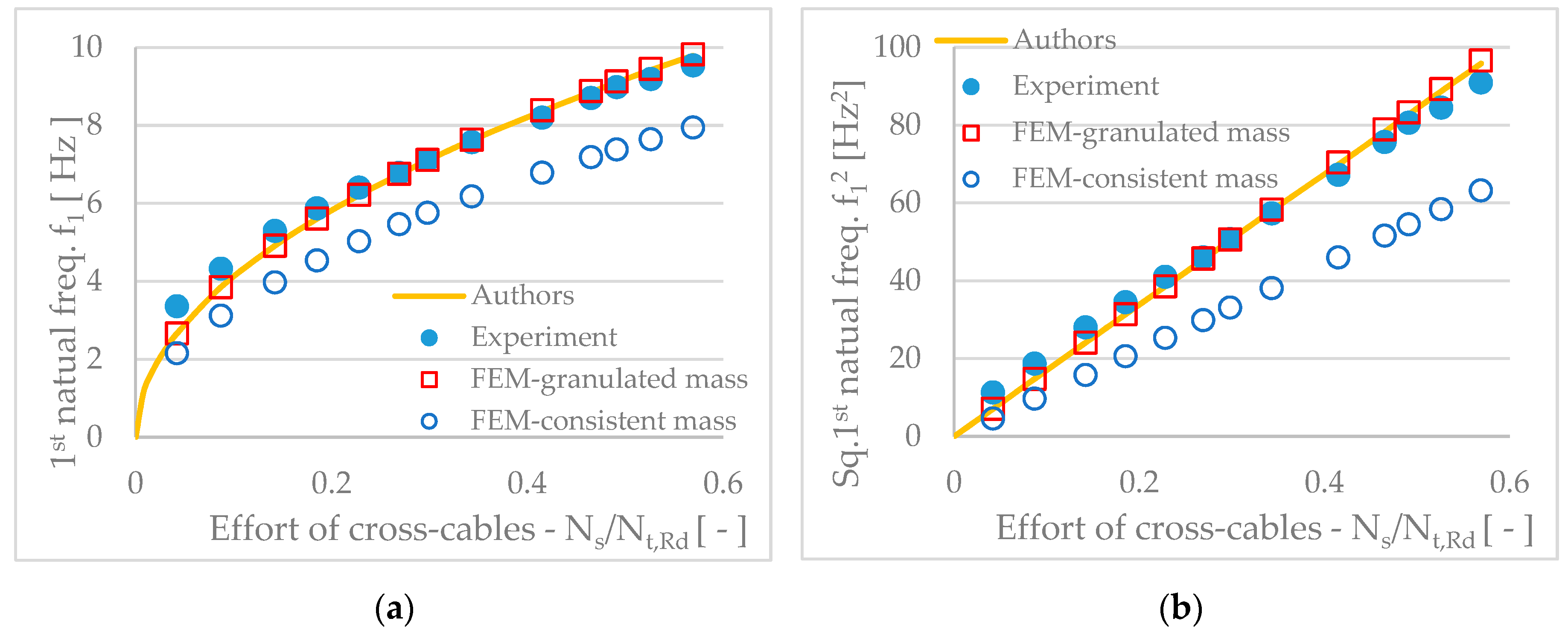
where the effective torsional stiffness $K_t$(15₁) is written depending on the prestress tension force in the cross-cable $N_s=E_s{A}_s{p}_0$, the mass moment of inertia about the simplex vertical axis for the three nodal masses is $I_0=m_r{L}_{}^2$ and $m_r$ denotes the reduced mass of one node. Figure 9 presents the comparison between the experimental results and the formula (16) and the results from the FEM. Additionally, the relationship between the square frequency and the force in the cross-cable is shown. The curve (16) is fitted into the experimental results by means of the curve fitting procedure performed in Matlab [28]. The excellent fit is achieved for the reduced mass $m_r=0.5m_n$, where the mass of the one node $m_n$ is calculated by dividing the weight of the experimental model by six. In the curve fitting procedure, the formula (16) was treated as a parametric equation with the mass $m_r$ as the parameter. The fitting procedure was constructed by changing the mass $m_r$ to match the theoretical solution (16) to the experimental data. The non-linear least-squares fitting procedure was used, in which the best fit was found for the sum of squares to errors $SSE=1.144$ and for the square of the multiple correlation the R-square $R_{sq}=0.9745$. The statistics SSE is indicating a better fit with a value closer to zero. For the R-square statistics the better the fit, the closer the values to one. The sensitivity of the frequency to the self-stress state is high enough to be successfully used to control the dynamic properties of the simplex.

The results from the FEM are presented for a lumped-mass idealization of the finite element mass matrix with the diagonal terms $m_r=0.5m_n$ and for the consistent-mass formulation with the calculated effective mass of the cables based on the weight of the experimental model. Very good agreement with formula (16) and with the experiment was found for the lumped-mass approach. In the case of the consistent-mass approach, the agreement is worse, although the change of the frequency has similar, non-linear characteristics during the prestress in the experiments and FEM calculations. In the FEM calculations the first frequency increases in proportion to the square root of the prestress force in the cross-cable. The difference between the experiments and numerical calculations for the consistent mass matrix decreases with the increase of the prestressing from approximately 60% for the first level through 30% for the fourth to 20% for the 13th level. For the level greater than 1.5 kN the difference is less than 25%, which may be acceptable at the moment, considering the very complex mass distributions in the physical model. It was observed in the experiments when the structure was not prestressed, the gravity caused heavy elements such as nodes to create a little prestress, which is not taken into account in the numerical analysis. Considering both the FEM calculation, quite good agreement was found between results of the finite element method and experimental tests.

It seems that the external loads should act similar to the prestressing. They cause the additional prestress. However, their effect should be greater with the lower prestress level due to the fact that with the increase of the prestressing the member forces caused by the external load gradually decrease relative to the prestress and their effect on the vibration frequency decreases.

Although non-linear analysis should be used to calculate the static load response of the tensegrity structure, the dynamic response can often be linearized around the equilibrium state corresponding to a designed prestress level and small vibrations can be analyzed. It was shown in the paper that the natural frequencies and modes of the simplex can be obtained using the experimental modal analysis approach. Also, usage of the finite element method in numerical simulations, allows to control the stiffness by regulating the level of pre-stressing. However, practice shows that there are some difficulties and an experimental validation can bring useful information, especially if the natural frequencies of the structure are measured and filtered from the whole experimental vibration spectrum.

The effect of self-stress on the overall stiffness of the tensegrity simplex was shown experimentally. The tendency of increasing the first natural frequency with an increase of the prestressing is clear visible in the experiments. It was also shown that adjustment of self-stress levels by means of the prestressing can also be used to control the dynamic properties of tensegrity simplex as the structures with one infinitesimal mechanism.

The vulnerability of tensegrities to dynamic excitation can be an important design issue due to their slenderness and lightness. The experimental validation of designed parameters, in particular modal ones, is essential for proper design in terms of load-bearing capacity and serviceability. Moreover, it serves as a quality control indicator for structural health monitoring purposes.

References

1. Skelton, R.E.; de Oliveira, M.C. Tensegrity Systems, 1st ed.; Springer: New York, NY, USA, 2009. [Google Scholar]
2. Gough, M. In the Laboratory of Constructivism: Karl Ioganson’s Cold Structures. JSTOR 1998, 84, 90. [Google Scholar] [CrossRef]
3. Heartney, E.; Snelson, K. Kenneth Snelson—Art and Ideas; Kenneth Snelson in association with Marlborough Gallery: New York, USA. Available online: http://kennethsnelson.net/KennethSnelson_Art_And_Ideas.pdf (accessed on 6 November 2020).
4. Snelson, K. Snelson On The Tensegrity Invention. Int. J. Space Struct. 1996, 11, 43–48. [Google Scholar] [CrossRef]
5. Motro, R. Tensegrity: Structural Systems for the Future; Kogan Page Science: London, UK, 2003. [Google Scholar]
6. Fraternali, F.; Carpentieri, G.; Amendola, A. On the mechanical modeling of the extreme softening/stiffening response of axially loaded tensegrity prisms. J. Mech. Phys. Solids 2015, 74, 136–157. [Google Scholar] [CrossRef] [Green Version]
7. Amendola, A.; Carpentieri, G.; De Oliveira, M.C.; Skelton, R.; Fraternali, F. Experimental investigation of the softening–stiffening response of tensegrity prisms under compressive loading. Compos. Struct. 2014, 117, 234–243. [Google Scholar] [CrossRef] [Green Version]
8. Małyszko, L. Static response of axially loaded tensegrity prism—Example of Using Proprietary Programming Language. In Lightweight Structures in Civil Engineering. Contemporary Problems XXII; Małyszko, L., Tarczewski, R., Eds.; University of Warmia and Mazur: Olsztyn, Poland, 2016; pp. 43–48. [Google Scholar]
9. Małyszko, L. Design of Tensegrity Modules with UHMWPE Cables Based on Experiments and Nonlinear Behaviour. In Lightweight Structures in Civil Engineering. Contemporary Problems XXIII; Gołębiowska, I., Dutkiewicz, M., Eds.; UTP University of Science and Technology: Bydgoszcz, Poland, 2017; pp. 25–30. [Google Scholar]
10. Małyszko, L.; Rutkiewicz, A.; Bilko, P. Dynamic Response of a Tensegrity Simplex in Impact Hammer Tests. In Lightweight Structures in Civil Engineering. Contemporary Problems XXIV; Kamiński, M., Szafran, J., Eds.; Łódź University of Technology: Łódź, Poland, 2018; pp. 69–75. [Google Scholar]
11. Motro, R.; Najari, S.; Jouanna, P. Static and Dynamic Analysis of Tensegrity Systems. Lect. Notes Eng. 1987, 26, 270–279. [Google Scholar] [CrossRef]
12. Ashwear, N.; Eriksson, A. Natural frequencies describe the pre-stress in tensegrity structures. Comput. Struct. 2014, 138, 162–171. [Google Scholar] [CrossRef]
13. Oppenheim, I.J.; Williams, W.O. Vibration of an elastic tensegrity structure. Eur. J. Mech. A/Solids 2001, 20, 1023–1031. [Google Scholar] [CrossRef]
14. Murakami, H. Static and dynamic analyses of tensegrity structures. Part 1. Nonlinear equations of motion. Int. J. Solids Struct. 2001, 38, 3599–3613. [Google Scholar] [CrossRef]
15. Chen, Y.; Feng, J. Initial prestress distribution and natural vibration analysis of tensegrity structures based on group theory. Int. J. Struct. Stab. Dyn. 2012, 12, 213–231. [Google Scholar] [CrossRef]
16. Nishimura, Y.; Murakami, H. Initial shape-finding and modal analyses of cyclic frustum tensegrity modules. Comput. Methods Appl. Mech. Eng. 2001, 190, 5795–5818. [Google Scholar] [CrossRef]
17. Oppenheim, I.J.; Williams, W.O. Vibration and Damping in Three-Bar Tensegrity Structure. J. Aerosp. Eng. 2001, 14, 85–91. [Google Scholar] [CrossRef]
18. Amouri, S.; Averseng, J.; Quirant, J.; Dubé, J.-F. Structural design and control of modular tensegrity structures. Eur. J. Environ. Civ. Eng. 2014, 19, 687–702. [Google Scholar] [CrossRef]
19. Averseng, J.; Dubé, J.-F.; Crosnier, B.; Motro, R. Active control of a tensegrity plane grid. In Proceedings of the 44th IEEE Conference on Decision and Control, Seville, Spain, 15 December 2006. [Google Scholar]
20. Ali, N.B.H.; Smith, I.F.C. Dynamic behavior and vibration control of a tensegrity structure. Int. J. Solids Struct. 2010, 47, 1285–1296. [Google Scholar] [CrossRef]
21. Obara, P. Monograph nr M116 - Dynamic and Dynamic Stability of Tensegrity Structures; Wydawnictwo Politechniki Świętokrzyskiej: Kielce, Poland, 2019. (In Polish) [Google Scholar]
22. Kasprzak, A. Assessment of the possibility of using tensegrity structures in bridge construction. Ph.D. Thesis, Warsaw University of Technology, Warsaw, Poland, 2014. (In Polish). [Google Scholar]
23. Kłosowska, J. Validation of using tensegrity structures in civil engineering structures. Ph.D. Thesis, Warsaw University of Technology, Warsaw, Poland, 2018. (In Polish). [Google Scholar]
24. Al Sabouni-Zawadzka, A.; Gilewski, W. Inherent Properties of Smart Tensegrity Structures. Appl. Sci. 2018, 8. [Google Scholar] [CrossRef] [Green Version]
25. Cosco, F.; Serratore, G.; Gagliardi, F.; Filice, L.; Mundo, D. Experimental Characterization of the Torsional Damping in CFRP Disks by Impact Hammer Modal Testing. Polymers 2020, 12. [Google Scholar] [CrossRef] [PubMed] [Green Version]
26. Chi, Y.; Dai, W.; Lu, Z.; Wang, M.; Zhao, Y. Real-Time Estimation for Cutting Tool Wear Based on Modal Analysis of Monitored Signals. Appl. Sci. 2018, 8. [Google Scholar] [CrossRef] [Green Version]
27. Reiterer, D.D.T.M.; Lachinger, S.; Fink, U.D.J.; Bruschetini-Ambro, S.-Z. In-Situ Experimental Modal Testing of Railway Bridges. Proceedings 2018, 2, 413. [Google Scholar] [CrossRef] [Green Version]
28. MathWorks Inc. Matlab Programming Fundamentals; The MathWorks, Inc.: Natick, MA, USA, 2020; Available online: https://ch.mathworks.com/help/pdf_doc/matlab/matlab_prog.pdf (accessed on 6 November 2020).
29. Reynders, E.; Schevenels, M.; de Roeck, G. Macec 3.3—A Matlab Toolbox for Experimental and Operational Modal Analysis—User’s Manual; KU Leuven—Structural Mechanics Section: Leuven, Belgium, 1997–2014; pp. 120–127. [Google Scholar]
30. Micro-Measurements. Tech Note TN-505-6—Strain Gage Selection: Criteria, Procedures, Recommendations; Micro-Measurements: Wendell, NC, USA , 2018; Available online: http://www.vishaypg.com/docs/11055/tn505.pdf (accessed on 6 November 2020).
31. Teac Corporation. Recording Unit LX-100 Series Instruction Manual; Teac Corporation: Tokyo, Japan, 2010. [Google Scholar]
32. PCB Piezotronics, Vibration Division. Instruction and Operating Manual of the Model 356B18 ICP Accelerometer; PCB Piezotronics, Inc.: Depew, NY, USA, 1999. [Google Scholar]
33. PCB Piezotronics. Instruction and Operating Manual of the Model 086C03 ICP Impact Hammer; PCB Piezotronics, Inc.: Depew, NY, USA, 2003. [Google Scholar]
34. Guillaume, P.; Verboven, P.; Vanlanduit, S.; Van Der Auweraer, H.; Peeters, B. A poly-reference implementation of the least-squares complex frequency-domain estimator. In Proceedings of the 21th Conference & Exposition on Structural Dynamics, Society for Experimental Mechanics, Kissimmee, FL, USA, 3–6 February 2003. [Google Scholar]
35. Oppenheim, I.; Williams, W. Geometric Effects in an Elastic Tensegrity Structure. J. Elast. 2000, 59, 51–65. [Google Scholar] [CrossRef]
Figure 1. Reference configuration of the tensegrity simplex: (a) tensegrity column; (b) spatial view the tensegrity simplex; (c) top view of the tensegrity simplex φ = 5 π / 6 .
Applsci 10 08733 g001
Figure 2. The model of the simplex: (a) the view; (b) details of the nodes; (c) the force transducer.
Applsci 10 08733 g002
Figure 3. The vibration measurement: (a) the standpoint with accelerometers in the top; (b) notation and directions of the strikes applied to upper nodes.
Applsci 10 08733 g003
Figure 4. The experimental distribution of member forces for the prestress levels: (a) the 4th level; (b) the 13th level.
Applsci 10 08733 g004
Figure 5. The identified type of the natural modes for all prestress levels: (a) the rotational mode; (b) the flexural mode.
Applsci 10 08733 g005
Figure 6. The acceleration in the frequency domain read from the 4th node at directions x (upper), y (central) and z (lower) for striking direction at azimuth: (a) 120 degrees and (b) 330 degrees.
Applsci 10 08733 g006
Figure 7. The acceleration in time domain, the acceleration in frequency domain, the power spectral density (PSD) of the acceleration in frequency domain of the signal 4x induced by the azimuth 240 degree impulse strike for: (a) the prestress level 4; (b) the prestress level 13.
Applsci 10 08733 g007
Figure 8. The stabilization diagram for the 4th level of the prestress, 4x direction of acceleration signal and the impulse at node P4 in direction: (a) 120 degrees and (b) 330 degrees.
Applsci 10 08733 g008
Figure 9. The effect of the prestress level on: (a) the first natural frequency; (b) the square of the first natural frequency.
Applsci 10 08733 g009