Article

MIMO LS-SVR-Based Multi-Point Vibration Response Prediction in the Frequency Domain

1
College of Computer Science and Technology, Huaqiao University, Xiamen 361021, China
2
College of Mechanical and Automation, Huaqiao University, Xiamen 361021, China
3
Department of Mathematics and Statistics, San Diego State University, San Diego, CA 92182, USA
*
Author to whom correspondence should be addressed.
Appl. Sci. 2020, 10(24), 8784; https://doi.org/10.3390/app10248784
Submission received: 26 October 2020 / Revised: 27 November 2020 / Accepted: 4 December 2020 / Published: 8 December 2020
(This article belongs to the Special Issue Nondestructive Testing (NDT): Volume II)

Abstract

:
To predict the multi-point vibration response in the frequency domain when the uncorrelated multi-source loads are unknown, a data-driven and multi-input multi-output least squares support vector regression (MIMO LS-SVR)-based method in the frequency domain is proposed. Firstly, the relationship between the measured multi-point vibration response and unmeasured multi-point vibration response is formulated using the transfer function in the frequency domain. Secondly, the data-driven multiple regression analysis problem of multi-point vibration response prediction in the frequency domain is described formally, and its mathematical model is established. With the measured multi-point vibration response as the input and the unmeasured multi-point vibration response as the output, the vibration response history data are assembled as a MIMO training dataset at each frequency. Thirdly, using the MIMO LS-SVR algorithm and MIMO history training dataset, the multi-point vibration response prediction model is built at each frequency point. By comparing the transmissibility matrix method, multiple linear regression model-based method, and MIMO neural network method, the application scope of the proposed method and its advantages are analyzed. The experimental results for acoustic and vibration experiment on a cylindrical shell verified that the MIMO LS-SVR-based method predicts the multi-point vibration response effectively when the loads are unknown, and has higher precision than the transfer function method, multiple linear regression method, MIMO neural network method, and transmissibility matrix method.

1. Introduction

Excessive vibration is one of the main reasons for the structural damage of a mechanism. It is necessary to predict the vibration response exactly, particularly for the area of machinery, buildings, bridges, and aerospace structures [1,2]. Vibration response prediction methods can be divided into the time domain and frequency domain, which was the first to be studied and is the most mature [3]. At present, traditional methods of multi-point vibration response prediction in the frequency domain for structures are all based on multiple loads excitation and structural characteristics. The main methods include following categories [4,5]: (1) equation deduction and theoretical analytical solution; (2) experimental test-and-measure methods; (3) simulation and numerical calculations, such as finite element analysis; and 4) data-driven multiple regression analysis prediction models.
Because they solve the ordinary differential or partial differential vibration equation, equation deduction and theoretical analytical solution methods [6,7] are only adapted to simple continuum structures (e.g., beam, plate and shell) and are powerless for complex structures.
In the experiments and measure methods [8,9,10], the multiple loads and transfer functions together determine the multi-point vibration response of the mechanical structure. As part of the structural characteristics, transfer functions between multiple loads excitation and multi-point vibration response are obtained in the transfer function experiment. For example, the response function of the system in the frequency domain can be acquired by simultaneously measuring the input spectrum function of the system’s multiple loads excitation and the output spectrum of the multi-point vibration response [11].
When transfer function or frequency response function between loads excitation and vibration response is unknown, the vibration response of the linear time-invariant (LTI) structure can also be acquired by finite element methods (FEM). By discretizing the vibration structure and considering the appropriate boundary conditions and connection conditions, it is easy to determine the multi-point vibration response of complex structures under complex loads excitation [7]. If the model is reasonable, more satisfactory vibration response prediction results can be obtained.
With recent further research on multiple regression analysis prediction models, the development of data-driven vibration response prediction methods is at the highest level of activity [12,13,14,15]. Wu [16] used least squares methods for vibration response prediction. However, if the system has suffered ill-posed problems, the prediction performance is often poor. Uddin [17] used an artificial neural network to predict the response of an offshore floating structure. However, because of the poor performance of the neural network in small-sample experiments and because many super-parameters need to be set, it is not easy to obtain a good prediction model. Support vector regression (SVR) has high prediction accuracy on small training samples and is not easy to overfit. By replacing nonequality constraints with equality constraints in SVR optimization, least squares-SVR (LS-SVR) reduces the high time complexity of the SVR algorithm. LS-SVR also solves the primal-dual problem, and it can replace the quadratic programming problem in SVR by solving a system of linear equations (caused by linear constraints in the optimization objective), and be applied to the regression task in high-dimensional input spaces. Many multiple regression analysis prediction models are essentially optimization problems. They seek the optimal solution for a certain goal using traditional optimization methods, such as gradient descent methods and Newton iterative methods, and fall easily into the local optimal solution [18,19]. To find the global optimal solution for these multiple regression analysis prediction models, the application of intelligent optimization algorithms is also a major trend at present. For example, the use of the particle swarm optimization algorithm to determine the optimal solution of LS-SVR to replace the SVR using traditional gradient descent methods for response prediction is described in [20,21]. Moreover, some response prediction methods have been developed in special fields, such as aeroelasticity and rotorcraft [22,23,24].
At present, most research is focused on vibration response prediction under the condition of known multiple loads excitation [25,26,27,28,29,30]. However, multiple loads excitation is often very difficult to measure and unknown in reality. For the study of response prediction under an unknown load, Zhu [31] solves the response prediction under the single load unknown condition. In the multi-point vibration response prediction problem under the condition of unknown uncorrelated multi-source loads, researchers [32,33,34,35,36,37] have used the transmissibility matrix to build a relationship between the unmeasured multi-point vibration response and measured multi-point vibration response, and predict the unmeasured vibration responses using the transmissibility matrix. However, the transmissibility matrix or transfer function of the LTI structure is often very difficult to obtain. When the transmissibility matrix or transfer function of the LTI structure is unknown, Zhan [38] used the measured vibration response based multiple linear regression model to predict the unmeasured vibration response in the frequency domain without the information of loads. Although this method can achieve good prediction results, the prediction accuracy is often affected by ill-posed problems at resonance frequencies. Multi-input multi-output least squares SVR (MIMO LS-SVR) methods can effectively alleviate the above problems [39].
Therefore, based on the above research, using the measured multi-point vibration response to predict the unmeasured multi-point vibration response in the frequency domain using MIMO LS-SVR methods is proposed.
The main innovations of this study are as follows:
(1)
In the case of unknown uncorrelated multiple loads excitation and transfer functions, the relationship between measured multi-point vibration response and unmeasured multi-point vibration response is derived. Then, the response prediction model based on data is established by using response history data.
(2)
Using the measured vibration response to predict the unmeasured vibration response in the frequency domain using MIMO LS-SVR methods is proposed. Its theoretical correctness, solvability, and applicability are discussed by comparing it with the transmissibility matrix, transfer function with known uncorrelated multi-source loads methods, multiple linear regression methods, MIMO neural network, and MIMO LS-SVR with known loads methods.

2. MIMO LS-SVR-Based Vibration Response Prediction under Unknown Uncorrelated Loads

2.1. Theoretical Inference of the Relationship between Multi-Point Vibration Responses

The problem we study is how to predict the vibration response of some locations which cannot be measured by using the known vibration response under unknown uncorrelated multi-source loads in the frequency domain. For a linear time invariant (LTI) dynamic structure in the frequency domain, the vibration response is split into two parts: measured vibration responses and unmeasured vibration responses. The measured vibration response means the vibration response value could be measured, and the vibration response value is known; the unmeasured vibration response means that the vibration response value is unknown, and is to be predicted in the model. n vibration responses can be classified into n 1 measured vibration response points y m s ( ω ) [ y 1 ( ω ) , y 2 ( ω ) , , y j ( ω ) , y n 1 ( ω ) ] , j = 1 , 2 , , n 1 , and n 2 unmeasured vibration response points y u m s ( ω ) [ y n 1 + 1 ( ω ) , y n 1 + 2 ( ω ) , , y n 1 + h ( ω ) , y n 1 + n 2 ( ω ) ] , h = 1 , 2 , , n 2 , where n 1 + n 2 = n .
For an LTI dynamics structure in the frequency domain, under the condition that m multi-source loads f ( ω ) [ f 1 ( ω ) , f 2 ( ω ) , , f i ( ω ) , f m ( ω ) ] are an uncorrelated random process with zero mean and second-order multiple-joint stationary characteristics, the relationship between the self-power spectrum s f f ( ω ) [ s f 1 f 1 ( ω ) , s f 2 f 2 ( ω ) , , s f i f i ( ω ) , s f m f m ( ω ) ] T of the loads f ( ω ) and the self-power spectrum s y y _ m s ( ω ) [ s y 1 y 1 ( ω ) , s y 2 y 2 ( ω ) , , s f j f j ( ω ) , s y n 1 y n 1 ( ω ) ] T of the vibration response y m s ( ω ) can be expressed as [38]
s y y _ m s ( ω ) = H m s ( ω ) s f f ( ω )
where
H m s ( ω ) [ | H 1 , 1 ( ω ) | 2 | H 1 , i ( ω ) | 2 | H 1 , m ( ω ) | 2 | H j , 1 ( ω ) | 2 | H j , i ( ω ) | 2 | H j , m ( ω ) | 2 | H n 1 , 1 ( ω ) | 2 | H n , 1 i ( ω ) | 2 | H n 1 , m ( ω ) | 2 ] ,
H j , i ( ω ) , i = 1 , 2 , , m , j = 1 , 2 , , n 1 denotes the frequency characteristics of the transfer function from input f i ( ω ) to response y j ( ω ) , and | H j , i ( ω ) | 2 is the modulo square of H j , i ( ω ) . ω = Δ f , 2 Δ f , , l Δ f , , Ω Δ f . Δ f is the frequency resolution. Ω is the total number of frequencies.
Using the least squares generalized inverse for Equation (1), an estimate s ^ f f ( ω ) of the self-power spectrum s f f ( ω ) can be obtained from the self-power spectrum s y y _ m s ( ω ) and H m s ( ω ) :
s ^ f f ( ω ) = ( H m s T ( ω ) H m s ( ω ) ) 1 H m s T ( ω ) s y y _ m s ( ω ) H m s ( ω ) + s y y _ m s ( ω )
Similarly, for the LTI structure in the frequency domain, the relationship between the self-power spectrum s f f ( ω ) of the loads f ( ω ) and the self-power spectrum s y y _ u m s ( ω ) [ s y n 1 + 1 y n 1 + 1 ( ω ) , s y n 1 + 2 y n 1 + 2 ( ω ) , , s f n 1 + h f n 1 + h ( ω ) , s y n 1 + n 2 y n 1 + n 2 ( ω ) ] T of the vibration responses y u m s ( ω ) [25] is
s y y _ u m s ( ω ) = H u m s ( ω ) s f f ( ω )
where
H u m s ( ω ) [ | H n 1 + 1 , 1 ( ω ) | 2 | H n 1 + 1 , i ( ω ) | 2 | H n 1 + 1 , m ( ω ) | 2 | H n 1 + h , 1 ( ω ) | 2 | H n 1 + h , i ( ω ) | 2 | H n 1 + h , m ( ω ) | 2 | H n 1 + n 2 , 1 ( ω ) | 2 | H n 1 + n 2 , i ( ω ) | 2 | H n 1 + n 2 , m ( ω ) | 2 ] ,
Substituting Equation (2) into Equation (3):
s y y _ u m s ( ω ) = H u m s ( ω ) s f f ( ω ) H u m s ( ω ) H m s ( ω ) + s y y _ m s ( ω )
When H u m s ( ω ) , H m s ( ω ) , and s y y _ m s ( ω ) are known, the s y y _ u m s ( ω ) can be obtained using Equation (4). The frequency characteristics of the transfer function H j , i ( ω ) j = 1 , 2 , , n 1   i = 1 , 2 , , m and H n 1 + h , i ( ω ) h = 1 , 2 , , n 2   i = 1 , 2 , , m can be obtained by experiment or the FEM method [36]. In this study, the experimental method is carried out through multi-point excitation to obtain transfer function. In order to get the transfer function, we need to collect the historical data of the load. The transfer function from a load point to a response point can be obtained by single point excitation, and then the transfer function from this point to all response points can be obtained by changing the position of the response measuring point. Then, we can move to another load point to give excitation and repeat the above actions to obtain all the transfer functions of the LTI structure.

2.2. Data-Driven Multiple Regression Analysis Problem Description of Multi-Point Vibration Response Prediction under Unknown Uncorrelated Multi-Source Loads

Let D ( ω ) H u m s ( ω ) H m s ( ω ) + n 2 × n 1 . Thus, Equation (4) can be rewritten as
s y y _ u m s ( ω ) D ( ω ) s y y _ m s ( ω )
When D ( ω ) n 2 × n 1 
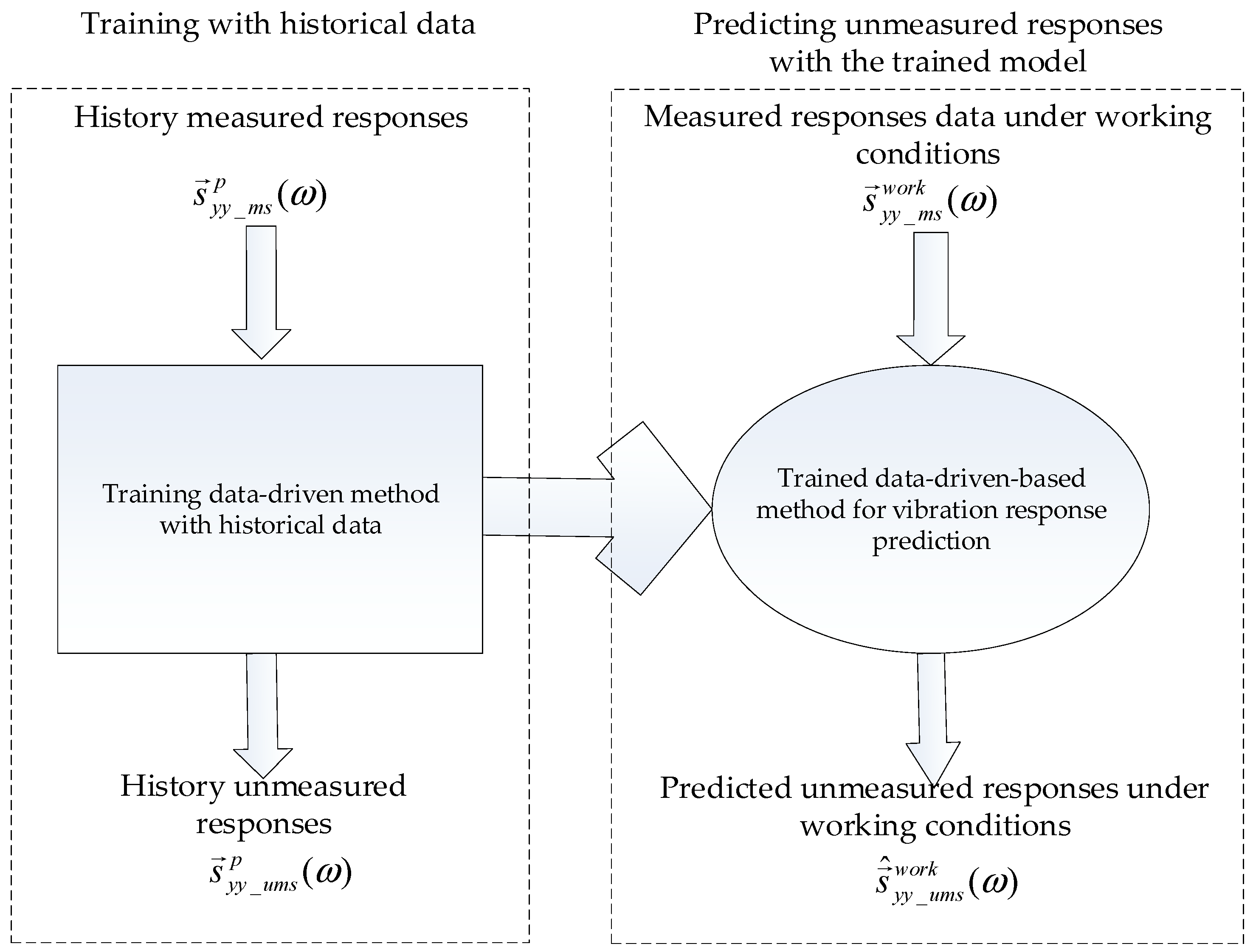
cannot be obtained using transfer functions and least squares generalization, it can be obtained using the history training dataset and a data-driven multi-point vibration response prediction model. Using the measured multi-point vibration response in Equation (3) as the input directly and the unmeasured multi-point vibration response as the output, a multi-input and multi-output multi-point vibration response prediction model for an LTI dynamics structure under unknown uncorrelated multi-source loads can be established using the history training dataset and multiple linear regression model. As shown in Figure 1, after training, the model can be used to predict the unmeasured vibration response in reality.
As shown in Figure 1, the history measured vibration response s y y _ m s p ( ω ) is the input and the history unmeasured vibration response points s y y _ u m s p ( ω ) are the output, p = 1 , 2 , , P , where P is the number of training samples. Similarly, from the historical data for each frequency ( ω = 1 , 2 , , l , , Ω , Ω is the total number of frequencies), the multi-point vibration response prediction model can be built for every frequency using multiple regression analysis, such as multiple linear regression model, MIMO neural network, or LS-SVR.
After the model is trained, the multi-point vibration response prediction model can be used to predict the unmeasured multi-point vibration response in a real-work condition. The measured multi-point vibration responses s y y _ m s w o r k ( ω ) are the input of the MIMO model, and the output of the model s ^ y y _ u m s w o r k ( ω ) is the predicted unmeasured multi-point vibration response data.
Clearly, the greater the amount of the history dataset that is used to train the data-driven multi-point vibration response model, the better the results the model acquires for all multiple regression analysis methods.

2.3. Procedure for Building and Applying the MIMO LS-SVR-Based Multi-Point Vibration Response Prediction Model

It can be seen from Section 2.2 that when D ( ω ) cannot be obtained, the problem can be transformed into a data-driven problem. The data-driven problem for an LTI structure can be solved using a MIMO LS-SVR with a linear or nonlinear kernel function. Thus, the next step is to use MIMO LS-SVR to acquire the complex relation D ( ω ) for each frequency.
LS-SVR [40,41] is a regression prediction model, which is developed and improved from Support vector machine (SVM). It is widely used in classification, numerical estimation, and density estimation. Its basic principle is to map the inputs into the high-dimensional space through the kernel function, and then find a hyperplane in the high-dimensional space to build a regression model in the hyperplane.
In the linear model, the predicted response S ^ y y _ u m s ( ω ) can be expressed as Equation (6), and the prediction model can be obtained by solving W ( ω ) .
S ^ y y _ u m s ( ω ) = W ( ω ) S y y _ m s ( ω ) + b 0 ( ω )
where S ^ y y _ u m s ( ω ) [ s y y _ u m s 1 ( ω ) , s y y _ u m s 2 ( ω ) , , s y y _ u m s p ( ω ) , , s y y _ u m s P ( ω ) ] , W ( ω ) is [ n 2 × n 1 ] matrix of regression coefficients, S y y _ m s ( ω ) [ s y y _ m s 1 ( ω ) , s y y _ m s 2 ( ω ) , , s y y _ m s p ( ω ) , , s y y _ m s P ( ω ) ] , b 0 ( ω ) is [ n 2 × 1 ] vector of model offset.
SVR uses a kernel function to map S y y _ m s ( ω ) to a high dimensional feature space to obtain the kernel matrix K ( ω ) :
K ( ω ) = ( k 1 , 1 ( ω ) k 1 , P ( ω ) k P , P ( ω ) k P , P ( ω ) )
k ( ω ) is the kernel function. In this study, the radial basis function (RBF) kernel function is used.
k i , j ( ω ) = exp ( s i y y _ u m s ( ω ) s j y y _ u m s ( ω ) 2 2 σ ( ω ) 2 )
where σ ( ω ) means the kernel width parameter.
The solution of LS-SVR problem can be solved by constructing Lagrange function to solve its corresponding linear Karush–Kuhn–Tucker (KKT):
[ b 0 ( ω ) B ( ω ) ] [ 0 I P Τ ( ω ) I p ( ω ) K ( ω ) + γ ( ω ) I p ( ω ) ] = [ 0 S y y _ u m s ( ω ) ]
where I p ( ω ) is a [ P × n 2 ] vector of ones, γ ( ω ) is a weight vector, and B ( ω ) represents regression vector.
It can be seen from Equations (8) and (9) that LS-SVR has two hyper-parameters ( σ ( ω ) , γ ( ω ) ) .
The [ b 0 ( ω ) B ( ω ) ] in LS-SVR can be obtained by training the model with a training set, and then LS-SVR can be used to predict the response under a real-work condition.
The procedure for building and applying the MIMO LS-SVR-based multi-point vibration response prediction in the frequency domain is shown in Figure 2.
(1)
With the measured multi-point vibration responses as the input and the unmeasured multi-point vibration responses as the output, the multi-point vibration response prediction model can be established using the historical training dataset and MIMO LS-SVR.
(2)
After training, the model can be used to predict the unmeasured vibration response under a real-work condition.

2.4. Theoretical Comparison of Response Prediction Methods

The computation of the condition number of transfer function matrix H ( ω ) is given by
c o n d ( H ( ω ) ) = | | H ( ω ) Τ H ( ω ) | | | | ( H ( ω ) Τ H ( ω ) ) 1 | |
For nearby resonance frequencies, the condition number of the transfer function matrix H ( ω ) is very large. Moreover, there exists an ill-conditioned part in the least squares generalized inverse of the transfer function matrix [36].
The least squares generalized inverse is needed in the transfer function method and the transmissibility matrix method. The least squares generalized inverse is also needed in the multiple linear regression methods. Because of the existence of an ill-conditioned part in the least squares generalized inverse, the transmissibility matrix and multiple linear regression are not robust to the measurement error, particularly for nearby resonance frequencies.
However, because there are no ill-conditioned parts or a need to use the least squares generalized inverse to calculate the transfer function matrix, using the measured multi-point vibration response to predict the unmeasured multi-point vibration response in the frequency domain using MIMO LS-SVR methods is robust for measurement noise. Simultaneously, the MIMO neural network [42] also has the above advantages, but the neural network requires many samples and hyperparameters to improve the prediction performance, and it is easy to overfit. It is not easy for the MIMO neural network to achieve a good prediction in small sample experiments. Therefore, MIMO LS-SVR is more suitable for response prediction in this study.
The comparison of the different methods are shown in Table 1.

2.5. Application Scopes of the Proposed Methods

The system in this paper needs to satisfy the following conditions:
(1)
This method can only be used in frequency domain, but not in time domain.
(2)
The structure must be linear time invariant. Otherwise, it is impossible to convert the data from time domain to frequency domain.
(3)
The locations of multiple load points must be unchanged; the loads applied at each load point are stationary with stable random excitation.
(4)
The history data of the measured multi-points’ response and the unmeasured multi-points’ response are needed. The locations of response points must be known. Because the location is different, the response will change accordingly. The number of measured multi-points must be greater than or equal to the number of loads, which means n 1 > m .

3. Experimental Verification

3.1. Acoustic and Vibration Experimental Devices on a Cylindrical Shell

The experimental device was a cylindrical shell structure. The cylindrical shell structure was fixed on a vibration table using a fixture and hung using elastic rubber ropes as shown in Figure 3a. There was an acoustic reverberation acoustic excitation (including an acoustic excitation sensor) in the interior of the cylindrical shell, as shown in Figure 3b. Additionally, the vibration table (including a vibration excitation sensor) on the exterior was the source of the vibration excitation, as shown in Figure 3c. Figure 3d shows the layout diagram for the measured vibration response. The position and direction of the vibration excitation of the vibration table and external acoustic reverberation of the acoustic excitation were fixed in each experiment, and the sensor response measuring point can reflect the main vibration of the system. In the experiments, a single spherical noise excitation source and a single suspended vibration table excitation were respectively applied to the device, and 18 measuring points were selected to record the response data.

3.2. Experimental Design and Data Processing

3.2.1. Data Acquisition

In this experiment, the vibration magnitudes of the spherical noise excitation source and suspension vibration excitation sources of different magnitudes were combined to obtain data of different independent and irrelevant experiments, and the response data of the system under all different conditions were taken as sample data. The acoustic stimulator had three orders of magnitude and the vibration stimulator had five orders of magnitude. The level of each load was not the same, and the signal generator controlled the excitation platform and spherical sound source. The uncorrelated multiple loads excitation and measuring multi-point positions were unchanged.
Therefore, there were 15 groups of combined stimuli with acoustic and vibration union independent loads. All the data collected were used as the entire sample data.

3.2.2. Fourier Transform of the Vibration Response Data

The data were first transformed from the time domain to the frequency domain using a fast Fourier transform. Thus, frequency data with a frequency from 0 Hz to 6400 Hz were obtained and the frequency resolution Δ f was 4 Hz. Then, based on the frequency resolution, the total number of frequencies Ω was 1601 groups.

3.2.3. Split of the Measured and Unmeasured Vibration Response Points

In this experiment, the 8th group was taken as the test set, and the other 14 groups as the training set. There were 18 vibration response measured points. n 1 measured vibration response multi-point data were chosen as the input and n 2 unmeasured response points’ data ( n 1 + n 2 = n ) were chosen as the output to train the MIMO LS-SVR model, where n denotes the total number of points’ responses used in the model. As discussed above, the number of measured points responses should be less than or equal to the training set sample. To satisfy the constraint of the applicable scope, n was 18. When multiple responses were predicted at the same time, the number of measured points was 16 and the number of unmeasured points was 2.

3.3. Evaluation Index

To validate the correctness and precision of the proposed methods, the predicted response must be compared with the real response; the 3 dB relative error is widely used for this in engineering practice. Given predicted response s ^ f n 1 + h f n 1 + h ( l Δ f ) and real response s f n 1 + h f n 1 + h ( l Δ f ) , to satisfy the 3 dB relative error, the condition is
10 log 10 | s ^ f n 1 + h f n 1 + h ( l Δ f ) s f n 1 + h f n 1 + h ( l Δ f ) | 3   a n d   10 log 10 | s f n 1 + h f n 1 + h ( l Δ f ) s ^ f n 1 + h f n 1 + h ( l Δ f ) | 3
For each frequency ω ( ω = Δ f , 2 Δ f , , l Δ f , , Ω Δ f , where Δ f is the frequency resolution and Ω is the total number of frequencies), the predicted response and true response did not satisfy Equation (7), which was recorded as a frequency 3 dB error. The percentage of the frequency 3 dB error was taken as the percentage of 3 dB.
In order to evaluate the prediction performance of the whole model, the mean absolute percentage error (MAPE) and root mean square error (RMSE) were also used to evaluate the model. The formulae are as follows:
M A P E = 1 Ω l = 0 Ω | ( s f n 1 + h f n 1 + h ( l Δ f ) s ^ f n 1 + h f n 1 + h ( l Δ f ) ) | s f n 1 + h f n 1 + h ( l Δ f )
R M S E = l = 1 Ω ( s f n 1 + h f n 1 + h ( l Δ f ) s ^ f n 1 + h f n 1 + h ( l Δ f ) ) 2 Ω
The smaller the RMSE and MAPE, the closer the predicted value is to the true value.

3.4. Parameter Settings of the MIMO LS-SVR Regression Prediction Model

For each frequency, a MIMO LS-SVR prediction model must be built. Additionally, in this experiment, the frequency value was between 0 Hz and 6400 Hz, and the frequency resolution Δ f was 4 Hz. Hence, the total number of different frequencies Ω was 1601. Thus, 1601 MIMO LS-SVR models had to be built.
The MIMO LS-SVR uses an RBF kernel function. Additionally, to obtain the best value of the hyperparameters (for LS-SVR, they were σ and γ ), a grid search method was applied to obtain the most suitable parameter values, in which we first tested several combination values, then set a range around the best combination value, and then grid searched within the range. The parameters of the penalty and regularization terms were optimally solved using a grid search, and the obtained gamma was 20.0 and sigma was 49.5. The experimental results of the vibration response prediction based on MIMO LS-SVR were obtained for the above parameters.

3.5. Comparison of Results among Different Multi-Point Vibration Response Prediction Methods

In order to verify the model performance of MIMO LS-SVR-based method, it was compared with the transmissibility matrix based method, transfer function with load based method (a method for predicting vibration response using known load and transfer function), multiple linear regression (MLR)-based method, MIMO neural network-based method (layers: 16-64-32-2, activation function: Rectified Linear Unit (ReLU), loss: MSE, epochs: 50, optimizer: Root Mean Square prop(RMSprop), learning rate: 0.0001, batch size: 2) and MIMO LS-SVR with load-based method (prediction of vibration response from known load using MIMO LS-SVR).
Table 2 shows the percentage of the number of frequencies whose energy prediction error was over 3 dB for different methods, where t1 and t2 represent two predicted vibration responses in the MIMO model. Figure 4 shows the energy dB of the true vibration response and predicted vibration response, the results within two horizontal lines indicate that the errors between the predicted results and the real results do not exceed 3 dB.
Table 3 shows the RMSE value of predicted vibration response in different methods, and Table 4 shows the MAPE value of predicted vibration response in different methods.
In order to verify the influence of different number of measurement points on accuracy, different number of measurement responses were selected to predict the unmeasured responses of point 1 and point 5 under different levels of noise. The results are shown in Table 5:
In order to verify the anti-noise ability of the method when there are few measured points, the two points measured response (equal to the number of uncorrelated load sources) is selected to predict the unmeasured responses of point 1 and point 5 under different levels of noise. The noise formula is s y y ( ω ) n o i s e = s y y ( ω ) ( 1 + n o i s e _ l e v e l r a n d ( 1 , 1 ) ) , where r a n d produces a random number in the range (−1, 1), and n o i s e _ l e v e l is the level of noise. The results are shown in Table 6:

3.6. Experimental Result Analysis of the Response Prediction

(1)
The natural resonance frequencies of the system can be obtained by detecting the peak values at high fluctuations of the response. The condition numbers of the structure’s frequencies around the natural resonance frequencies are shown in Table 7. As shown in Table 7 and Figure 4, because of the large condition number, the frequencies of the multi-point vibration response prediction error over 3 dB of data were mainly near the resonance frequencies.
(2)
As shown in Table 2, Table 3 and Table 4, the predicted multi-point vibration response of MIMO LS-SVR-based methods was very close to the real multi-point vibration response, and the average error over 3 dB was approximately 1%. The average error over 3 dB of the methods that predicted the unmeasured multi-point vibration response using the measured multi-point vibration response (transmissibility matrix, MIMO LS-SVR) was better than the methods that predicted the unmeasured multi-point vibration response using known loads (transfer function with loads and MIMO LS-SVR with loads) at most points, which indicates that the prediction methods that predict the unmeasured response using the measured response still have good prediction performance when the uncorrelated multi-source loads are unknown, even better than some methods for predicting response using known loads.
(3)
Compared with the MIMO neural network method and MLR, the predictive performance of MIMO SVR is much higher than that of MIMO NN and MLR, because these three methods predict the unknown response with known response when the load is unknown, so it can be seen from the Table 2, Table 3 and Table 4 that SVR is more suitable for the application in this situation.
(4)
As shown in Figure 4 and Table 2, Table 3 and Table 4, MIMO LS-SVR-based method has the best result compared with other methods on the indicators of the over 3 dB and MAPE, indicating that the predictive ability of MIMO LS-SVR-based method is better than that of other methods on the indicators of relative error; and on RMSE, MIMO LS-SVR-based method also has a good predictive effect. Although it was not as high as that for the transmissibility matrix-based methods, the MIMO LS-SVR-based method predicted a response without the transmissibility matrix and regardless of whether the structures were linear or nonlinear.
(5)
It can be seen from Table 5 that the fewer the measurement points, the worse the accuracy of the LS-SVR model, but even if there are only two measurement points (equal to the number of uncorrelated load sources), the LS-SVR model can still maintain high accuracy. Moreover, it is found from Table 6 that the LS-SVR model can maintain high performance even when there is only one measurement point, which indicates that the LS-SVR model has high applicability.

4. Conclusions

In this paper, a novel problem was proposed: how to use the measured multi-point vibration response to predict the unmeasured multi-point vibration response in the frequency domain under unknown uncorrelated multi-source loads using data-driven multiple regression analysis. After completing the problem description, the solution of this problem was presented, which was an MIMO LS-SVR-based multi-point vibration response prediction model using the measured multi-point vibration response and the unmeasured multi-point vibration response history training dataset. The experimental verification results for acoustic and vibration sources on union loads experimental devices on a cylindrical shell demonstrated that this proposed approach is more effective and has higher accuracy than transmissibility matrix-based methods and multiple linear regression model-based multi-point vibration response prediction methods.
Because this method cannot be used when the measurement position is unknown, in the next step, we can study how to predict the position and response simultaneously. If the multiple loads excitations are correlated with each other in the frequency domain, the relationship between the multiple loads excitation and vibration responses is much more complex, and the phase becomes very important. Moreover, due to the phase loss of this method, the predicted vibration response power spectrum of unknown points cannot be converted to the time domain. Therefore, phase information containing the multi-point dynamic random vibration response prediction algorithm in the frequency domain is a further research direction. Additionally, validating this method on nonlinear time invariant structures is also future work.

Author Contributions

Conceptualization, C.W., D.C., H.H. and W.Z.; methodology, C.W., D.C., H.H. and W.Z.; software, D.C., H.H. and W.Z.; validation, D.C., H.H. and W.Z.; writing—original draft preparation, D.C., H.H. and W.Z.; writing—review and editing, C.W., D.C., H.H. and W.Z.; supervision, C.W., X.L. and J.C.; project administration, C.W.; funding acquisition, C.W., X.L. and J.C.; Correspondence, C.W. All authors have read and agreed to the published version of the manuscript.

Funding

This research was funded by the National Natural Science Foundation of China grant numbers 51305142 and 51305143, the China Postdoctoral Science Foundation grant number 2014M552429 and the Promotion Program for Young and Middle-aged Teachers in Science and Technology Research at Huaqiao University grant number ZQN-PY212.

Conflicts of Interest

The authors declare no conflict of interest.

References

  1. Farrar, C.R.; Worden, K. An introduction to structural health monitoring. Philos. Trans. R. Soc. A Math. Phys. Eng. Sci. 2007, 365, 303–315. [Google Scholar] [CrossRef] [PubMed]
  2. Farrar, C.R.; Worden, K. Structural Health Monitoring: A Machine Learning Perspective; John Wiley & Sons: Hoboken, NJ, USA, 2012. [Google Scholar]
  3. Paik, I.; Roesset, J.M. Use of Quadratic Transfer Functions to Predict Response of Tension Leg Platforms. J. Eng. Mech. 1996, 122, 882–889. [Google Scholar] [CrossRef]
  4. Vicario, F.; Phan, M.Q.; Betti, R.; Longman, R.W. Output-only observer/Kalman filter identification (O3KID). Struct. Control Health Monit. 2014, 22, 847–872. [Google Scholar] [CrossRef]
  5. Marcello, M. Structural Damage Assessment through Parametric and Nonparametric Models. Ph.D. Thesis, Columbia University, New York, NY, USA, 2020. [Google Scholar]
  6. Albert, C.G.; Veronesi, G.; Nijman, E.; Rejlek, J. Prediction of the vibro-acoustic response of a structure-liner-fluid system based on a patch transfer function approach and direct experimental subsystem characterisation. Appl. Acoust. 2016, 112, 14–24. [Google Scholar] [CrossRef] [Green Version]
  7. Wu, Z.Z.; Liu, W.N.; Ma, L.X.; Wang, W.B. Prediction method for metro environmental vibrations based on measured frequency response functions. Eng. Mech. 2015. [Google Scholar] [CrossRef]
  8. Somashekar, V.; Harikrishnan, S.; Ahmed, P.A.; Kamesh, D. Vibration Response Prediction of the Printed Circuit Boards Using Experimentally Validated Finite Element Model. Procedia Eng. 2016, 144, 576–583. [Google Scholar] [CrossRef]
  9. Mao, W.; Tian, M.; Yan, G. Research of load identification based on multiple-input multiple-output SVM model selection. Proc. Inst. Mech. Eng. Part C J. Mech. Eng. Sci. 2011, 226, 1395–1409. [Google Scholar] [CrossRef]
  10. Wang, C.; Wu, Y.; Jiao, J.; Huang, X.; Gou, J.; Yan, G. Load Identification of Acoustic and Vibration Multi-source Following Linear Regression and Least-Squares of Generalized Matrix Inverse method in Frequency Domain. Sens. Transducers 2014, 168, 268–275. [Google Scholar]
  11. Wang, J.; Wang, C.; Zhong, B.; Wang, T.; Guo, W.; Chen, W.; Sun, C. Uncorrelated multi-sources load identification in frequency domain based on improved Tikhonov regularization method. Int. J. Appl. Electromagn. Mech. 2016, 52, 983–990. [Google Scholar] [CrossRef]
  12. Yinfeng, D.; Yingmin, L.; Ming, L.; Mingkui, X. Nonlinear structural response prediction based on support vector machines. J. Sound Vib. 2008, 311, 886–897. [Google Scholar] [CrossRef]
  13. Yin, Z.Y.; Sun, Y.D. A vibration response prediction method in frequency domain for liquid piping systems in vessels. J. Ship Mech. 2013, 17, 1352–1360. [Google Scholar] [CrossRef]
  14. Thormann, R.; Widhalm, M. Linear-Frequency-Domain Predictions of Dynamic-Response Data for Viscous Transonic Flows. AIAA J. 2013, 51, 2540–2557. [Google Scholar] [CrossRef]
  15. Wu, Z.; Liu, W.; Ma, L.; Wang, W. Frequency domain analytical method for predicting metro environmental vibration based on soil frequency response function. China Railw. Sci. 2014, 35, 105–112. [Google Scholar] [CrossRef]
  16. Wu, S.F.; Natarajan, L.K. Analysis of Vibro-acoustic Responses of a Complex Structure Using Helmholtz Equation Least Squares Based Nearfield Acoustical Holography. Chin. J. Automot. Eng. 2011, 1, 237–247. [Google Scholar]
  17. Uddin, A.; Jameel, M.; Razak, H.A.; Islam, A.B.M.S. Response Prediction of Offshore Floating Structure Using Artificial Neural Network. Adv. Sci. Lett. 2012, 14, 186–189. [Google Scholar] [CrossRef] [Green Version]
  18. Lian, J.; He, L.; Wang, H. Prediction of vibration response of powerhouse structures based on LS-SVR optimized by PSO. Eng. Sci. 2011, 13, 45–50. [Google Scholar] [CrossRef]
  19. Xu, G.B.; Han, W.W.; Wang, H.J. Vibration response prediction of a powerhouse structure based on SSPSO-GRNN. J. Vib. Shock 2015, 34, 104–109. [Google Scholar] [CrossRef]
  20. Hughes, K.; Campbell, J.; Vignjevic, R. Application of the finite element method to predict the crashworthy response of a metallic helicopter under floor structure onto water. Int. J. Impact Eng. 2008, 35, 347–362. [Google Scholar] [CrossRef] [Green Version]
  21. Hossain, A.; Humphrey, L.; Mian, A. Prediction of the dynamic response of a mini-cantilever beam partially submerged in viscous media using finite element method. Finite Elem. Anal. Des. 2012, 48, 1339–1345. [Google Scholar] [CrossRef]
  22. Patt, D.; Liu, L.; Friedmann, P.P. Rotorcraft Vibration Reduction and Noise Prediction Using a Unified Aeroelastic Response Simulation. J. Am. Helicopter Soc. 2005, 50, 95–106. [Google Scholar] [CrossRef]
  23. Sivasakthivel, P.S.; Velmurugan, V.; Sudhakaran, R. Prediction of vibration amplitude from machining parameters by response surface methodology in end milling. Int. J. Adv. Manuf. Technol. 2010, 53, 453–461. [Google Scholar] [CrossRef]
  24. Morse, T.L.; Williamson, C.H.K. Prediction of vortex-induced vibration response by employing controlled motion. J. Fluid Mech. 2009, 634, 5–39. [Google Scholar] [CrossRef]
  25. Tandon, N.; Choudhury, A. An analytical model for the prediction of the vibration response of rolling element bearings due to a localized DEFECT. J. Sound Vib. 1997, 205, 275–292. [Google Scholar] [CrossRef]
  26. Živanović, S.; Pavić, A.; Reynolds, P. Probability-based prediction of multi-mode vibration response to walking excitation. Eng. Struct. 2007, 29, 942–954. [Google Scholar] [CrossRef]
  27. Hollkamp, J.J.; Gordon, R.W.; Spottswood, S.M. Nonlinear modal models for sonic fatigue response prediction: A comparison of methods. J. Sound Vib. 2005, 284, 1145–1163. [Google Scholar] [CrossRef]
  28. Dalenbring, M. Validation of estimated isotropic viscoelastic material properties and vibration response prediction. J. Sound Vib. 2003, 265, 269–287. [Google Scholar] [CrossRef]
  29. Jones, C.A.; Pavic, A.; Reynolds, P.; Harrison, R.E. Verification of equivalent mass–spring–damper models for crowd–structure vibration response prediction. Can. J. Civ. Eng. 2011, 38, 1122–1135. [Google Scholar] [CrossRef]
  30. Chan, Y.-J.; Ewins, D.J. Prediction of Vibration Response Levels of Mistuned Integral Bladed Disks (Blisks): Robustness Studies. J. Turbomach. 2011, 134, 044501. [Google Scholar] [CrossRef]
  31. Zhu, C.C.; Wang, M.L.; Zeng, Q.M. Prediction of response of vibration environmental test based on vibration transfer feature. J. Southwest Jiaotong Univ. 2002, 37, 1–4. [Google Scholar] [CrossRef]
  32. Ribeiro, A.M.R.; Maia, N.M.M.; Silva, J.M.M. Response prediction from a reduced set of known responses using the transmissibility. In Proceedings of the 18th International Modal Analysis Conference (IMAC XVIII), San Antonio, TX, USA, 7–10 February 2000; pp. 425–427. [Google Scholar]
  33. Gajdatsy, P.; Janssens, K.; Desmet, W.; Van Der Auweraer, H. Application of the transmissibility concept in transfer path analysis. Mech. Syst. Signal Process. 2010, 24, 1963–1976. [Google Scholar] [CrossRef]
  34. Law, S.; Li, J.; Ding, Y. Structural response reconstruction with transmissibility concept in frequency domain. Mech. Syst. Signal Process. 2011, 25, 952–968. [Google Scholar] [CrossRef]
  35. Urgueira, A.P.V.; Almeida, R.A.B.; Maia, N.M.M. On the use of the transmissibility concept for the evaluation of frequency response functions. Mech. Syst. Signal Process. 2011, 25, 940–951. [Google Scholar] [CrossRef]
  36. Wang, Z.; Zhu, P. Response prediction for modified mechanical systems based on in-situ frequency response functions: Theoretical and numerical studies. J. Sound Vib. 2017, 400, 417–441. [Google Scholar] [CrossRef]
  37. Zhan, W.; Wang, C.; Zhang, H.; Lai, X.; Chen, Y. Transfer functions and loads identification based response prediction in situation of unknown uncorrelated multi-source loads. Int. J. Appl. Electromagn. Mech. 2019, 59, 1029–1039. [Google Scholar] [CrossRef]
  38. Wang, C.; Zhan, W. Multivariant linear regression model based response prediction in situation of unknown uncorrelated multiple sources load. Vibroeng. Procedia 2017, 14, 271–277. [Google Scholar] [CrossRef]
  39. Wu, Z.; Ding, C.; Li, G.; Han, X.; Li, J. Learning solutions to the source inverse problem of wave equations using LS-SVM. J. Inverse Ill Posed Probl. 2019, 27, 657–669. [Google Scholar] [CrossRef]
  40. Li, Y.; Shao, X.; Cai, W. A consensus least squares support vector regression (LS-SVR) for analysis of near-infrared spectra of plant samples. Talanta 2007, 72, 217–222. [Google Scholar] [CrossRef]
  41. De Magistris, M.; Di Bernardo, M.; Manfredi, S.; Petrarca, C.; Yaghouti, S. International Journal of Circuit Theory and Applications. Int. J. Circuit Theory Appl. 2016, 27, 605–615. [Google Scholar] [CrossRef]
  42. Zhu, C.C.; Wang, M.L.; Zeng, Q.M.; Wang, D.S. Neural network prediction for responses of random vibration environment tests. J. Vib. Shock 2007, 26, 42–45. [Google Scholar] [CrossRef]
Figure 1. Data-driven multi-point vibration response prediction under unknown uncorrelated multi-source loads.
Applsci 10 08784 g001
Figure 2. Procedure for building and applying the multi-input multi-output least squares support vector regression (MIMO LS-SVR)-based multi-point vibration response prediction model in the frequency domain under unknown uncorrelated multi-source loads.
Applsci 10 08784 g002
Figure 3. (a) Acoustic and vibration experimental devices. (b) Acoustic excitation. (c) Vibration excitation source. (d) Vibration response point layout diagram. (Reprinted from International Journal of Applied Electromagnetics and Mechanics, Vol 59, Wei Zhan et al., Transfer functions and loads identification based response prediction in situation of unknown uncorrelated multi-source loads, 1029–1039, No.3, Copyright (2020), with permission from IOS Press).
Applsci 10 08784 g003
Figure 4. Energy dB error of the different methods. (a) t1 = 1. MIMO LS-SVR. (b) t2 = 5. MIMO LS-SVR. (c) t1 = 1. MIMO LS-SVR with loads. (d) t2 = 5. MIMO LS-SVR with loads. (e) t1 = 1. Transmissibility matrix. (f) t2 = 5. Transmissibility matrix. (g) t1 = 1. Transfer function with loads. (h) t2 = 5. Transfer function with loads. (i) t1 = 1. Multiple linear regression (MLR). (j) t2 = 5. MLR. (k) t1 = 1. MIMO Neural network. (l) t2 = 5. MIMO Neural network.
Applsci 10 08784 g004aApplsci 10 08784 g004bApplsci 10 08784 g004c
Table 1. Comparison of the different methods.
MethodsTransmissibility MatrixTransfer Function with LoadMultiple Linear RegressionMIMO Neural NetworkMIMO LS-SVR
Comparison Index
Need transfer function or notYesYesNoNoNo
RobustnessMediumMediumBadGoodGood
Need to search for hyperparameters or notNoNoNoYesYes
Matrix inverse illnesses exist or notYesYesYesNoNo
ExplanatoryGoodGoodMediumBadBad
Time complexityGoodGoodMediumBadBad
Suitable for linear or nonlinear systemsLinear onlyLinear onlyLinear onlyBoth linear and nonlinearBoth linear and nonlinear
Table 2. Percentage of the number of frequencies whose energy prediction error is over 3 dB for different models (%).
Model t1t2t1t2t1t2
152689
Transmissibility matrix>3 dB1.310.443.250.691.121.37
<−3 dB1.060.370.750.751.191.06
total2.370.814.001.442.312.44
Transfer function with loads >3 dB1.751.374.561.871.872.00
<−3 dB1.811.561.251.941.501.50
total3.562.945.813.813.373.50
Multiple linear regression>3 dB1.441.695.251.751.621.75
<−3 dB3.944.316.934.623.945.37
total5.376.0012.186.375.567.12
MIMO Neural network>3 dB3.561.622.812.444.254.56
<−3 dB2.752.063.252.624.814.93
total6.313.696.065.069.069.49
MIMO LS-SVR with loads>3 dB1.871.753.622.442.252.44
<−3 dB0.310.310.120.560.370.19
total2.192.063.753.002.622.62
MIMO LS-SVR>3 dB0.560.252.250.500.690.94
<−3 dB0.120.000.810.120.120.19
total0.690.253.060.620.811.12
Table 3. Mean absolute percentage error (MAPE) of the predicted multi-point vibration response for different models.
Modelt1t2t1t2t1t2
152689
Transmissibility matrix0.178830.155980.510880.163460.178780.19932
Transfer function with loads0.229500.221840.508250.234030.233080.24108
MLR0.221130.235951.201810.234940.233650.24227
MIMO Neural network1.797560.298730.374600.327260.382010.45450
MIMO LS-SVR with loads0.223140.219730.396500.233720.228950.23774
MIMO LS-SVR 0.143600.145050.377150.150980.155140.16821
Table 4. Root mean square error (RMSE) of the predicted multi-point vibration response for different models.
Modelt1t2t1t2t1t2
152689
Transmissibility matrix0.015660.022200.015970.030560.007260.01261
Transfer function with loads0.025290.065620.029800.051010.017180.01667
MLR0.026310.021490.039830.054770.025240.03301
MIMO Neural network0.071720.127260.059260.056440.030490.03019
MIMO LS-SVR with loads0.033480.061370.025460.045230.017800.01565
MIMO LS-SVR0.016820.037230.020470.027040.009060.01653
Table 5. Performance of the MIMO LS-SVR model under different number of measurement points.
ModelIndex (Mean)24816
MIMO LS-SVR>3 dB1.440.590.530.41
<−3 dB0.280.220.160.06
total1.720.810.690.47
MAPE0.218140.181920.157270.14433
RMSE0.038950.029810.030460.02702
Table 6. Performance of the MIMO LS-SVR model under different level of noise.
ModelIndex (Mean)0%5%10%20%30%40%
MIMO LS-SVR>3 dB1.441.341.943.755.656.65
<−3 dB0.280.440.723.125.186.31
total1.721.782.656.8710.8412.96
MAPE0.218140.227600.257310.327550.377530.39701
RMSE0.038950.037560.051470.087840.091420.15710
Table 7. Condition number of the structure’s frequencies around natural resonance frequencies.
OrderFrequencies around Resonance Frequencies Condition Number
11005.6944
2132449.7810
3280188.3306
4332138.5945
553698.9278
65967.8165
786443.5228
892825.5819
912683.0790
1013363.2506
1114241.7005
1214447.2473
1316846.1383
14174412.0795
1518123.9039
1618647.0644
Publisher’s Note: MDPI stays neutral with regard to jurisdictional claims in published maps and institutional affiliations.

