Screening Patients with Early Stage Parkinson’s Disease Using a Machine Learning Technique: Measuring the Amount of Iron in the Basal Ganglia

Abstract

The purpose of this study was to determine whether a support vector machine (SVM) model based on quantitative susceptibility mapping (QSM) can be used to differentiate iron accumulation in the deep grey matter of early Parkinson’s disease (PD) patients from healthy controls (HC) and Non-Motor Symptoms Scale (NMSS) scores in early PD patients. QSM values on magnetic resonance imaging (MRI) were obtained for 24 early PD patients and 27 age-matched HCs. The mean QSM values in deep grey matter areas were used to construct SVM and logistic regression (LR) models to differentiate between early PD patients and HCs. Additional SVM and LR models were constructed to differentiate between low and high NMSS scores groups. A paired t-test was used to assess the classification results. For the differentiation between early PD patients and HCs, SVM had an accuracy of 0.79 ± 0.07, and LR had an accuracy of 0.73 ± 0.03 (p = 0.027). SVM for NMSS classification had a fairly high accuracy of 0.79 ± 0.03, while LR had 0.76 ± 0.04. An SVM model based on QSM offers competitive accuracy for screening early PD patients and evaluates non-motor symptoms, which may offer clinicians the ability to assess the progression of motor symptoms in the patient population.

1. Introduction

Effective screening for early Parkinson’s disease (PD) is essential, as early diagnosis and treatment can postpone the progression of symptoms and complications caused by the disease [1]. Early detection can also economically reduce the burden of elderly patients [2]. Despite the importance of early diagnosis, PD is still under-recognized in its early stages [3], perhaps partially because existing diagnostic criteria are mainly based on subjective symptoms [4]. Additionally, in the early stages of PD, nonmotor symptoms (NMS), such as olfactory problems, depression, and rapid eye movement sleep disorder, are more prominent than motor symptoms, further complicating the early diagnosis of this disease [3,5].

Recent studies have demonstrated that iron accumulation in the deep grey matter (e.g., the substantia nigra (SN), globus pallidus (GP), dentate nucleus (DN), red nucleus (RN), caudate nucleus (CN), and putamen (PUT)) may serve as a potential biomarker of PD [6,7,8]. Quantitative susceptibly mapping (QSM) on magnetic resonance imaging (MRI) may be useful in detecting this iron accumulation [9]. QSM uses the phase difference induced by differences in tissue susceptibility to estimate magnetic susceptibility. Because iron is the primary source of these susceptibility changes, QSM has been used in patients PD patients to measure iron distribution [8,10]. In this research, patients with PD demonstrated significantly increased QSM values in the basal ganglia areas than healthy volunteers [10]. Research has also shown that the amount and extent of iron deposition in the brain vary depending on the severity of disease [6]. Thus, QSM may prove valuable in the diagnosis of PD.

Recently, researchers have begun to assess the use of machine learning techniques for the diagnosis of PD. A support vector machine (SVM), one of the most potent classification algorithms based on machine learning techniques, has been used in such studies [11,12], demonstrating accuracy rates of 86% [12] and 97% [11] for the detection of moderately advanced PD in patients with atypical forms of parkinsonism using diffuse tensor imaging and susceptibility-weighted imaging each. However, these studies focused on patients with advanced PD; no previous studies have assessed the use of an SVM model to detect early PD.

Therefore, the purpose of this study was to assess the potential of machine learning-based screening for early PD. We constructed an SVM model using QSM values to distinguish between patients with early PD and healthy volunteers and compared them with those from logistic regression (LR) models. As non-motor symptoms and motor symptoms are related to the pathologic severity of PD [13], we constructed separate SVM and LR models to distinguish between patients with low Non-Motor Symptoms Scale (NMSS) scores and those with high NMSS scores.

2. Materials and Methods

The Institutional Review Board approved the study protocol of the Seoul National University-Seoul Metropolitan Government Boramae Medical Center (SNU-SMG Boramae Medical Center—IRB 26-2016-107, approval date: 22 September 2016). The requirement for informed consent was waived because the data were collected retrospectively.

2.1. Subjects

Twenty-four patients with early PD (16 women, 8 men; mean age, 69 years; range, 56–79 years) and 27 age-matched healthy controls (HCs) (20 women, 7 men; mean age, 65 years; range, 53–82 years) who had undergone 3 Tesla MRI (Achieva 3.0T, Koninklijke Philips N.V., Amsterdam, The Netherlands) were retrospectively recruited for this study. The clinical diagnosis of early PD was evaluated by movement disorder specialists (Chaewon Shin and Jee-Young Lee) based on United Kingdom brain bank criteria [14]. Disease duration of early PD was defined as the duration from the onset of motor symptoms (mean, 0.8 years; range, 0–3 years). The severity of PD was measured with Hoehn and Yahr stage and Movement Disorder Society-sponsored revision of the Unified Parkinson’s Disease Rating Scale (MDS-UPDRS) part II and III scores [15]. NMSS scores were evaluated with the Korean version of the NMSS (K-NMSS) [16]. HC patients with no neurological disease other than HC were selected. The demographic and clinical characteristics of early PD and HC are summarized in

Table 1. Demographic and clinical characteristics of the study cohort.

Characteristic	Patients with Early PD a (n = 24)	HCs b (n = 27)	p-Value
Mean age, years (range)	68.8 (56–79)	65.3 (53–82)	0.139 *
Sex (male:female)	8:16	7:20	0.759 †
Mean disease duration, years (range) ‡	0.8 (0–3)	-	-
Mean NMSS c score (range)	18 (4–47)	-	-
Mean Hoehn and Yahr stage (range)	1.6 (1–2.5)	-	-
Mean MDS-UPDRS d (part III sum) (range)	17.8 (4–40.5)	-	-

* p value from Student t-test. ^† p value from chi-square test. ^‡ Disease duration defined as duration from the onset of motor symptoms. ^a, PD = Parkinson’s disease, ^b, HC = healthy control, ^c, NMSS = Non-motor Symptoms Scale, ^d, MDS-UPDRS = Movement Disorder Society-sponsored revision of the Unified Parkinson’s Disease Ratings Scale.

. The 24 early PD patients data and 27 HC patients data were collected retrospectively from a study performed by Shin et al. [17].

2.2. MR Data Acquisition

All the participants were scanned with 3D gradient echo images using an Achieva 3T MR system (Philips, Amsterdam, The Netherlands). The scan parameters were: resolution, 0.4 × 0.4 × 2 mm³; 70 to 80 slices (to cover the whole brain); repetition time, 18.16 to 19.78 ms; echo time, 25.65 to 27.98 ms; matrix size, 512 × 512; flip angle, 10°; and the number of receiver channels in the head coil, 8. The 3D gradient echo images were then used directly for processing.

2.3. QSM Reconstruction

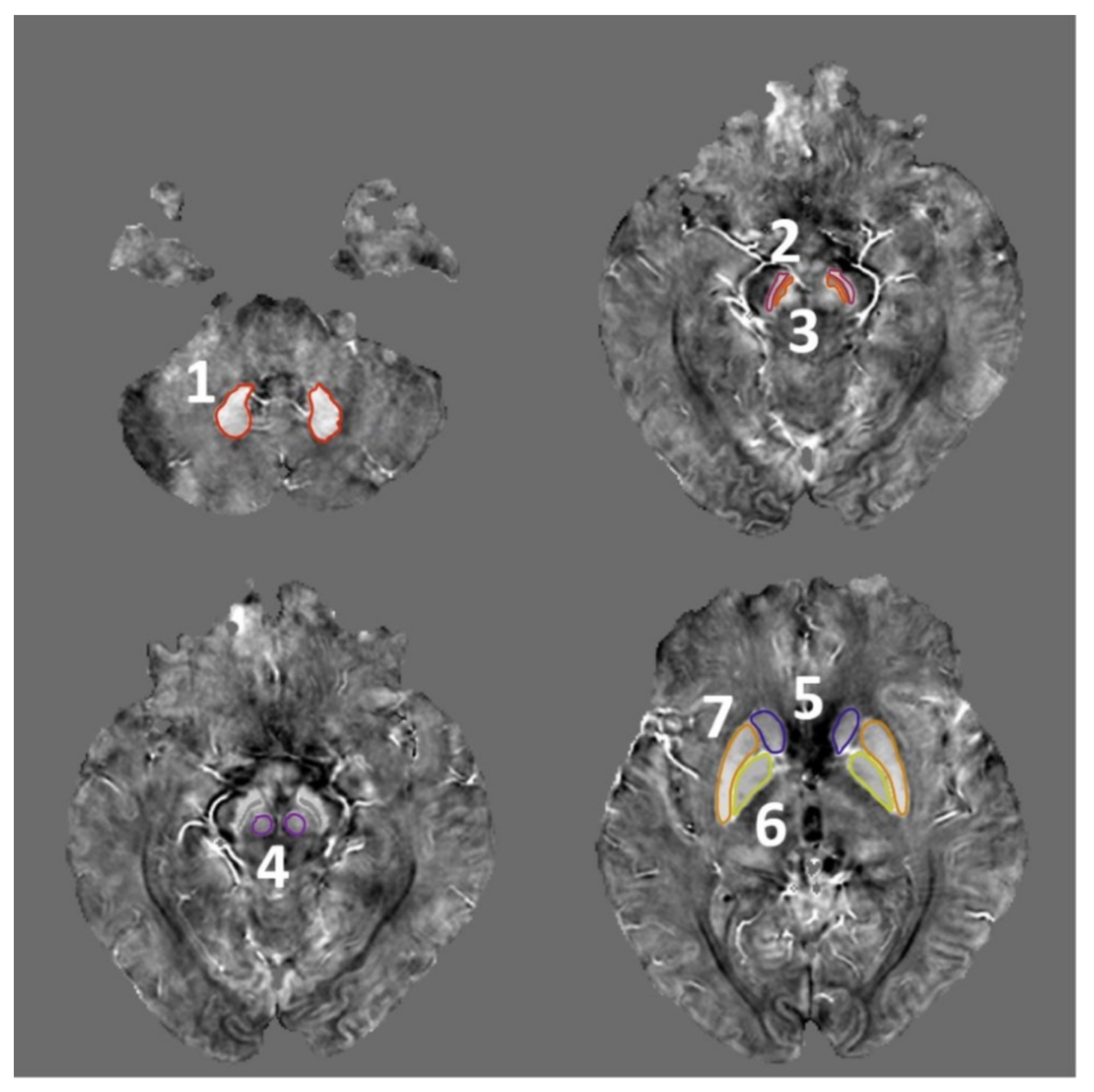
QSM was reconstructed with a susceptibility tensor imaging software suite (Version 2.2, Brain Imaging & Analysis Center, Durham, NC, USA). The process consisted of 3 steps. In the first step, the acquired phase map was unwrapped to a continuous phase image with HARmonic (background) PhasE Removal using the Laplacian operator (HARPERELLA) [18]. Because magnetic sources other than brain tissue (e.g., bone) can affect the obtained field, the second step involved removing the background field, originating from outside the tissue of interest [19]. These two steps were performed simultaneously by estimating the phase originating from the background and applying fast Fourier transform-based inverse Laplacian. In the third step, the magnitude image and tissue field from the first step were combined to reconstruct the QSM image. Because the inversion from k-space to field map is ill-conditioned due to the insufficiency of k-space values, magnetic susceptibility obtained from k-space includes streaking artifacts. Thus, we used the least-squares algorithm-based method to identify the artifacts and exclude them from obtained susceptibility maps.

2.4. ROI Selection

To obtain mean QSM values in deep gray matter, seven regions of interest (ROIs), including the CN, PUT, GP, SN pars compacta (SNc), SN pars reticulate (SNr), RN, and DN, were manually drawn on two to three adjacent slices of each reconstructed QSM image (Figure 1). We selected these seven ROIs because they are correlated with the pathogenesis and progression of PD [6]. The thalamus was excluded because it had a wider area than the other regions and was challenging to delineate uniformly on the images.

2.5. Classification Models

SVM is a powerful method for solving a two-class classification problem. The primary objective of SVM is to determine the hyperplane that maximizes the distance from each datum of different classes or margins [20]. The specific data nearest to the hyperplane and thus are most relevant to its construction are called support vectors. If the examples from different classes are severely overlapping, the input data dimension can be manipulated using Gaussian kernel functions to enhance the classification performance.

LR has been widely used for classification problems in the clinical field [21] and has become a gold standard for data analysis [22]. LR provides a model for estimating the dependence of a binary response variable, and this model can fit into an S curve using various methods. The LR model is based on the linear combination of predictors and is fitted using maximum likelihood estimation. Classification is accomplished by estimating probability to the set threshold.

In this study, the SVM and LR models were constructed using MATLAB R2014a (The MathWorks Inc., Natick, MA, USA).

2.6. Feature Selection

To achieve the optimal performance of SVM and LR models, backward elimination based on Fisher’s score (F-score) was used for the feature selection. F-score was calculated using the following equation:

$$\mathrm{F}\left(\mathrm{i}\right)= \frac{{\left({\overline{x_i}}^{(+)}-\overline{x_i}\right)}^2+{\left({\overline{x_i}}^{(-)}-\overline{x_i}\right)}^2}{\frac{1}{n_{+}-1}{{\displaystyle \sum }}_{k=1}^{n+}{\left(x_{k,i}{}^{(+)}-{\overline{x_i}}^{(+)}\right)}^2+\frac{1}{n_{-}-1}{{\displaystyle \sum }}_{k=1}^{n-}{\left(x_{k,i}{}^{(-)}-{\overline{x_i}}^{(-)}\right)}^2}.$$

(1)

In this equation, $\overline{x_i}$, ${\overline{x_i}}^{(+)}$, and ${\overline{x_i}}^{(-)}$ are the average QSM values of the ith feature of the whole, PD (positive), and HC (negative) datasets, respectively, and $x_{k,i}{}^{(+)}$ and $x_{k,i}{}^{(-)}$ are the kth QSM value of the ith feature for the positive and negative subjects, respectively. $n_{+}$ and $n_{-}$ represent the numbers of positive and negative subjects, respectively.

F-score measures the deviation between the two groups of real numbers [23]: a larger F-score represents a larger deviation. We included values from the ROI with the highest F-score to the ROI with the lowest F-score to apply backward elimination.

For a subclassification model, PD cases were divided into two groups based on the median NMSS score in study patients (15.5 ±11.5); when median NMSS was set as the threshold, the two groups were defined as high NMSS score (mean ± SD, 26.6 ± 10.0) and low NMSS score (mean ± SD, 9.4 ± 3.8). The F-scores of ROIs for these groups were compared.

2.7. Performance Assessment

Evaluation of the proposed method was based on accuracy, sensitivity, specificity, and area under the receiver operating characteristics curve (AUC). Accuracy was defined as the ratio of correctly diagnosed subjects to all subjects. Sensitivity was defined as the ability to detect true positives (early PD) as positives, and specificity was defined as detecting true negatives (HC) as negatives. The receiver operating characteristic curve was defined as the plot of the classification ability, with the x-axis representing the false-positive rate (1-specificity) and the y-axis representing the true positive rate (sensitivity). Theoretically, AUC would be in the range of 0.5 to 1, with an AUC of 1 representing the perfect classification result.

To evaluate the performance of SVM and LR, we applied two methods for classification models. The first method was to use all datasets to obtain average performance from 10-fold cross-validation. Because data distribution in folds for training and validation affects the performance of models due to the small number of datasets, data distribution was randomized 10 times and divided differently into folds. Thus, each cross-validation has different training and validation datasets. The average performance of models was calculated. The second method was to use 80% of datasets for training and 20% of datasets for the test. The training was performed to determine optimal features; datasets validated one time and training model with the optimal features. For NMSS classification models, data were not divided into training and test sets because the number of datasets is only 48. Instead, the first method was performed to evaluate the average performance of the NMSS models.

For SVM, the nested cross-validation was performed to measure the optimal performance. The nested cross-validation is used to search hyperparameters of the SVM model during cross-validation. The nested cross-validation consists of two folds: inner and outer folds. The inner fold determines the optimal hyperparameters of a classification model, changing the hyperparameters of the model iteratively. In the outer fold, the same dataset is applied to the classification model tuned with optimal hyperparameters to estimate generalization error [24].

A paired t-test was used to compare SVM and LR models’ results with the same number of features and compare the best SVM and LR models. Paired t-tests were used to assess the accuracy, sensitivity, specificity, and AUC of the models, and a p-value < 0.05 was considered significant.

3. Results

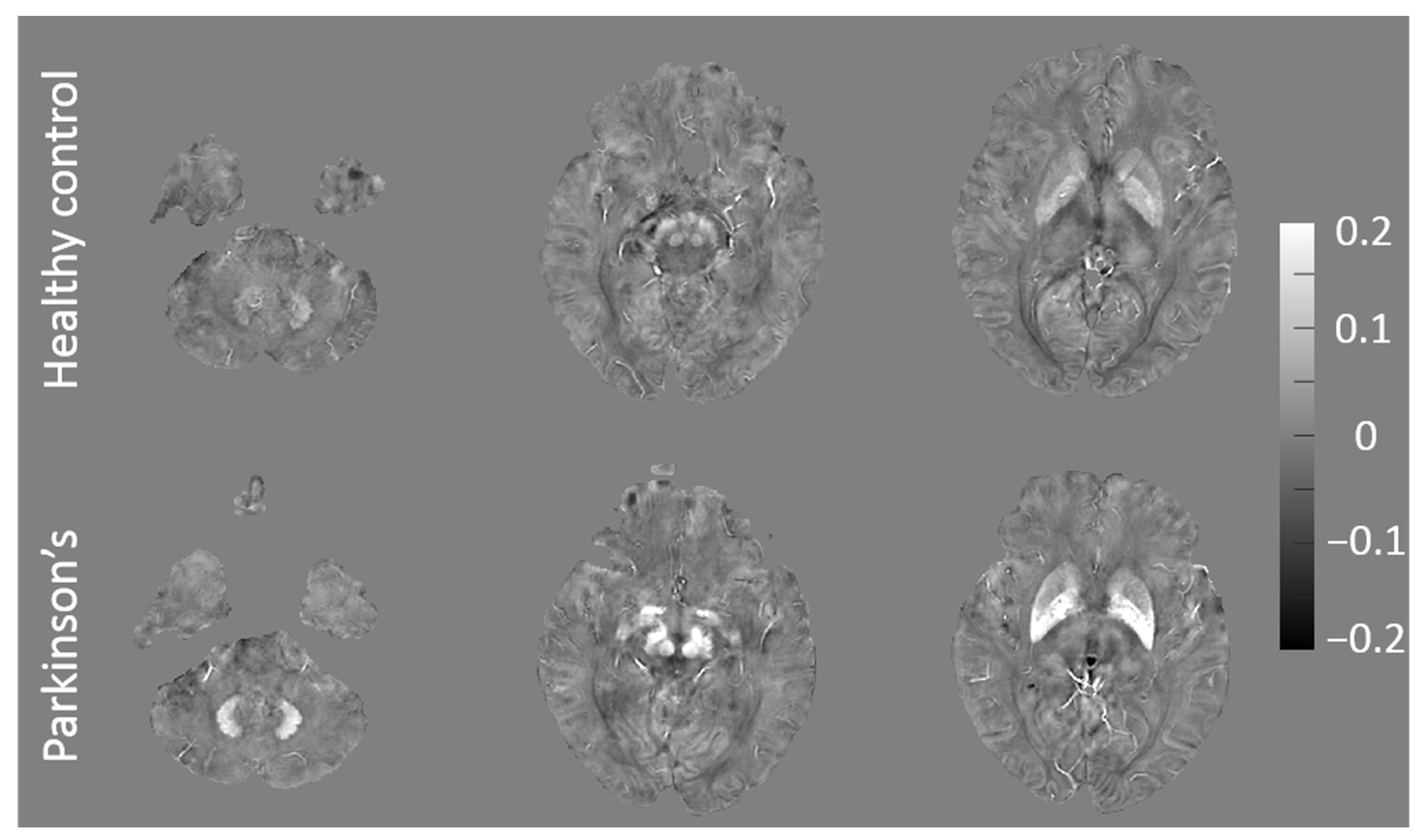
3.1. QSM and F-Scores for Patients with Early PD and HCs

Figure 2 shows representative QSM images of HC and early PD. By visual inspection, QSM images of early PD shows brighter signals in basal ganglia areas than HC, demonstrating iron accumulation in early PD.

Mean QSM values for the seven ROIs in patients with PD and HCs are shown in

Table 2. QSM Values and F-scores for Patients with Early PD ^a and HCs ^b.

ROI c	Mean QSM k Value ± SD, ppm		F-score l
	Patients with Early PD (n = 24)	HCs (n = 27)
GP d	0.142 ± 0.034	0.134 ± 0.038	14.634
DN e	0.101 ± 0.031	0.095 ± 0.026	11.461
SNr f	0.131 ± 0.044	0.115 ± 0.044	11.261
SNc g	0.130 ± 0.043	0.125 ± 0.041	9.349
RN h	0.102 ± 0.032	0.097 ± 0.034	9.251
CN i	0.070 ± 0.025	0.059 ± 0.021	7.497
PUT j	0.109 ± 0.049	0.094 ± 0.025	6.910

^a, PD = Parkinson’s disease, ^b, HC = healthy control, ^c, ROI = region of interest, ^d, GP = globus pallidus, ^e, DN = dentate nucleus, ^f, SNr = substantia nigra pars reticulate, ^g, SNc = substantia nigra pars compacta, ^h, RN = red nucleus, ⁱ, CN = caudate nucleus, ^j, PUT = putamen, ^k, QSM = quantitative susceptibility mapping, ^l, F-score = Fisher’s score.

. The mean QSM values for early PD patients were approximately 10% higher (range, 0.070–0.142 ppm) than the values for HCs (range, 0.059–0.134 ppm). In comparisons of F-scores for patients with PD and HCs, GP demonstrated the highest F-score, and PUT demonstrated the lowest, meaning that the largest difference between patients with PD and HCs was in the GP.

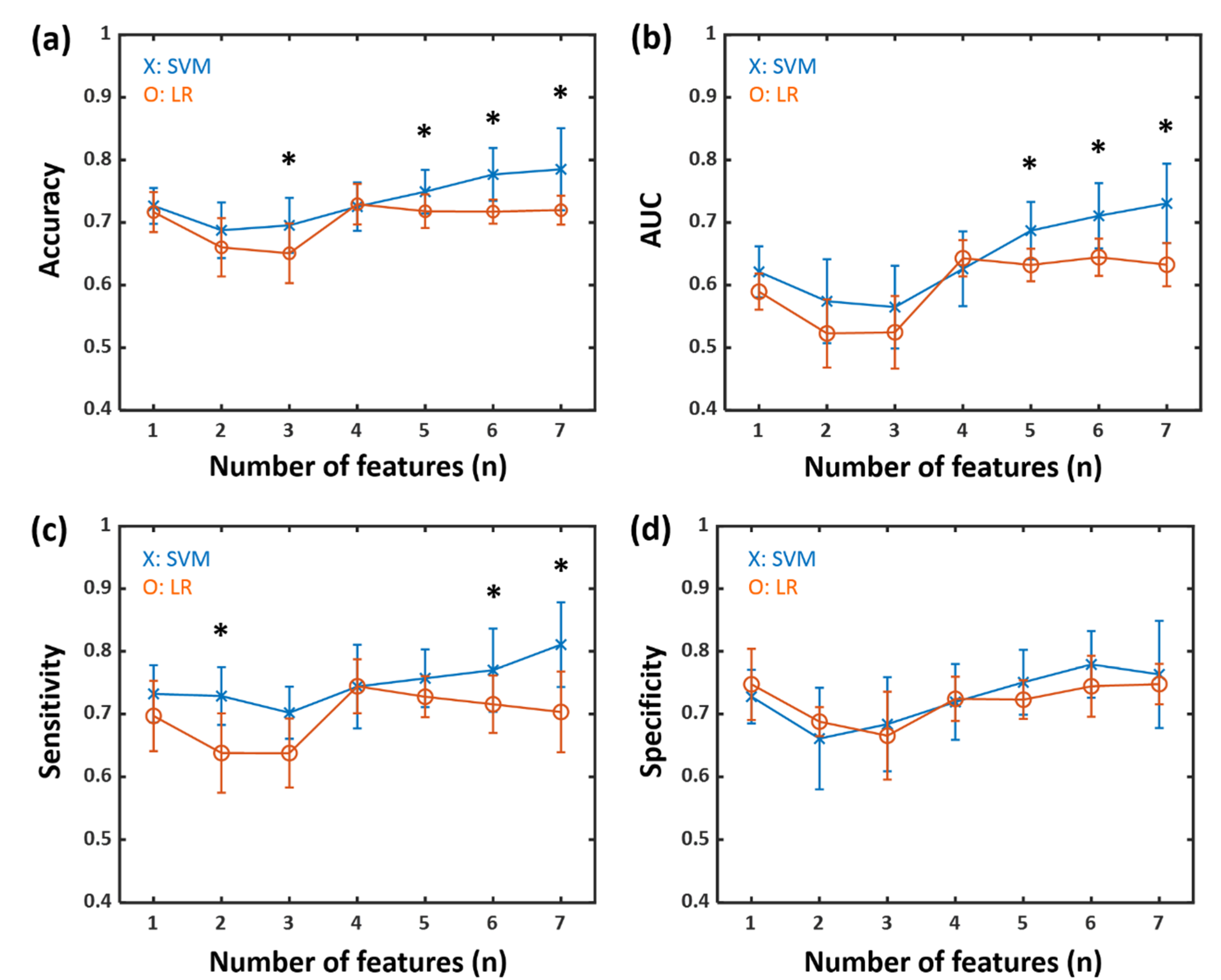
3.2. Classification Results for Patients with Early PD and HCs

When training and test datasets were not separated, backward elimination results based on F-score are shown in Figure 3. The best performance for SVM was observed when all seven ROIs were used. For LR, the best performance was observed when four features were used (GP, DN, SNr, and SNc).

When we compared the performance of the best SVM model (using GP, RN, DN, SNr, SNc, CN, and PUT) with LR models with the same features, the calculated p-value was less than 0.01 inaccuracy, AUC, and sensitivity, demonstrating a significant difference between the performance of the SVM model using all seven ROIs and the performance of LR models.

The optimal SVM model demonstrated accuracy, sensitivity, specificity, and AUC values of 0.79 ± 0.07, 0.81 ± 0.07, 0.76 ± 0.09, and 0.73 ± 0.06, respectively (Figure 3). The optimal LR model demonstrated accuracy, sensitivity, specificity, and AUC values of 0.73 ± 0.03, 0.74 ± 0.04, 0.72 ± 0.04, and 0.64 ± 0.03, respectively. SVM had approximately 10% higher accuracy than LR overall. The performance of the best SVM model was significantly different from that of the best LR model (p = 0.027 in accuracy, p = 0.001 in AUC, and p = 0.017 in sensitivity) except for specificity (p = 0.199).

Table 3. Classification results of SVM ^a and LR ^b from the training set.

	The Number of Features
		1	2	3	4	5	6	7
Accuracy
	SVM a	0.67	0.65	0.65	0.64	0.72	0.71	0.76
	LR b	0.58	0.55	0.59	0.70	0.69	0.70	0.72
AUC c
	SVM a	0.58	0.45	0.40	0.48	0.62	0.63	0.70
	LR b	0.40	0.37	0.36	0.59	0.58	0.62	0.64
Sensitivity
	SVM a	0.68	0.54	0.56	0.55	0.81	0.89	0.77
	LR b	0.49	0.49	0.52	0.69	0.62	0.64	0.72
Specificity
	SVM a	0.70	0.76	0.72	0.75	0.67	0.60	0.84
	LR b	0.69	0.67	0.68	0.75	0.82	0.79	0.72

^a, support vector machine, ^b, logistic regression, ^c, area under the receiver operating curve.

shows classification results from training data when separating datasets into training and test. The SVM model with all features shows the best performance (accuracy = 0.76, AUC = 0.70, sensitivity = 0.77, and specificity = 0.84), while LR has accuracy, AUC, sensitivity, and specificity of 0.72, 0.64, 0.72, and 0.72, respectively. When using all features for the SVM and LR models, in the test set, SVM revealed better accuracy (=0.8), AUC (=0.90), and sensitivity (=0.75) than those of LR (accuracy = 0.75, AUC = 0.64, and sensivity = 0.5) except for specificity (SVM = 0.88 and LR = 0.92). An LR model with GP, DN, SNr, and SNc selected in Figure 3 also had the same performance as the LR model with all features in the test set.

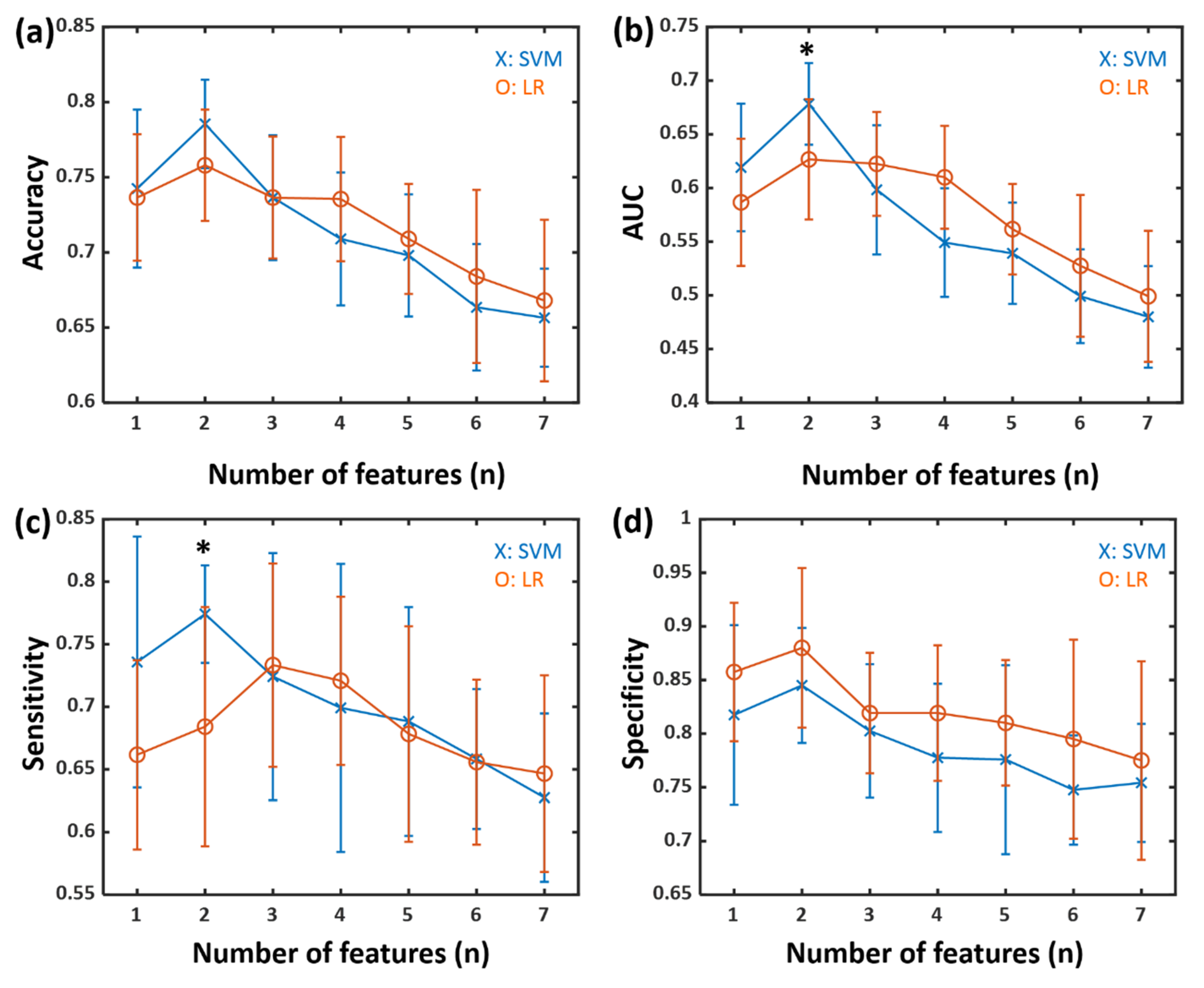
3.3. Classification Results for High and Low NMSS Score Groups

Mean QSM values for the high and low NMSS score groups are shown in

Table 4. QSM ^a values and F-scores ^b for patients with high or low NMSS ^c score.

ROI d	Mean QSM Value ± SD, ppm		F-score
	High NMSS (n = 12)	Low NMSS (n = 12)
GP e	0.136 ± 0.029	0.149 ± 0.037	17.772
RN f	0.106 ± 0.028	0.099 ± 0.035	10.544
DN g	0.102 ± 0.033	0.100 ± 0.031	10.426
SNr h	0.129 ± 0.043	0.133 ± 0.045	9.070
SNc i	0.127 ± 0.045	0.134 ± 0.042	9.063
CN j	0.074 ± 0.027	0.067 ± 0.023	7.846
PUT k	0.111 ± 0.042	0.107 ± 0.056	5.005

High and low Non-motor Symptoms Scale (NMSS) score groups were divided based on the median value of the NMSS within study patients (15.5). ^a, QSM = quantitative susceptibility mapping, ^b, F-scores = Fisher’s score, ^c, NMSS = non-motor symptoms scale, ^d, ROI = region of interest, ^e, GP = globus pallidus, ^f, RN = red nucleus, ^g, DN = dentate nucleus, ^h, SNr = substantia nigra pars reticulata, ⁱ, SNc = substantia nigra pars compacta, ^j, CN = caudate nucleus, ^k, PUT = putamen.

. The difference between QSM values in these groups was only 0.5% for all ROIs (high NMSS score group = 0.112 ± 0.02 ppm; low NMSS score group = 0.113 ± 0.03 ppm).

In terms of F-scores, GP again demonstrated the highest (17.772), and PUT again demonstrated the lowest (5.005) (Table 3). We implemented SVM and LR models for high and low NMSS score classification. The optimal features for the SVM and LR models were GP and RN. With the selected two ROIs, the SVM model demonstrated accuracy, sensitivity, specificity, and AUC values of 0.79 ± 0.03, 0.77 ± 0.04, 0.85 ± 0.06, and 0.68 ± 0.04, respectively, while the LR model showed those of 0.76 ± 0.04, 0.68 ± 0.10, 0.88 ± 0.07, and 0.63 ± 0.06, respectively (Figure 4).

When the optimal SVM model (using GP and RN) and the LR model (using GP and RN) were compared, p-values for sensitivity and AUC were < 0.05; the p value for accuracy and specificity were 0.09 and 0.525, respectively.

4. Discussion

Because early treatment of PD enhances patients’ quality of life, effective early screening methods are essential. Dopamine imaging and the assessment of alpha-synuclein levels in the blood or spinal fluid have been considered the standard screening tools, but these methods have limitations; for instance, dopamine imaging may lack cost competitiveness as a screening tool. Meanwhile, recent MRI studies have demonstrated that iron accumulation in the basal ganglia may serve as a potential biomarker of PD. In this study, we used QSM, a new MRI technique, to noninvasively measure iron accumulation in the brain and thus differentiate between patients with early PD and HCs. This technique demonstrated its ability to serve as a rapid machine learning-based screening tool in this patient population.

Early PD diagnosis is challenging, as only subtle symptoms appear in the early stages [25]. The SVM model constructed in this study had an accuracy of 79% for identifying early PD, an accuracy rate similar to that demonstrated by experienced neurologists using clinical criteria (approximately 76%) [26]. Therefore, this machine learning-based technique, therefore, offers a diagnostic accuracy rate comparable to that demonstrated by experienced neurologists but independent of the clinicians’ involved skills.

We found that QSM values were higher in patients with early PD than in HCs in all ROIs (GP, RN, DN, SNr, SNc, CN, and PUT). A previous study reported that iron accumulates in the basal ganglia (e.g., SNc) in patients with early PD and is progressively stored in nearby areas [6]. Our study also suggests that iron deposition in the deep grey matter may occur in early PD patients.

In this study, we found that GP demonstrated the highest F-score for differentiating between patients with early PD and HCs. A previous study of QSM values demonstrated that iron accumulation in GP is prevalent in early PD [6], and another study found a positive correlation between GP iron content and PD severity [27]. However, data regarding these potential correlations are still limited; further research is needed to investigate the importance of GP iron content in patients with early PD.

SVM has the best performance in discriminating early PD and HC when all features are used. The previous studies have demonstrated significant elevation of QSM values in basal ganglia regions such SNc, SNr, GP, or RN in PD, and the iron accumulation has a progressive pattern extending from SNc to adjacent basal ganglia regions as with the disease progression in patients with early PD [6,28,29]. In a perspective of classifying PD and HCs with SVM, this broad progressive pattern in the basal ganglia allows more information on constructing the classification model, resulting in better performance when using more features as shown in Figure 3.

SVM showed higher performance than LR. SVM uses a kernel function to transform datasets into the required form of data. Because data of this study has a high dimension, SVM with the kernel function is superior to deciding a hyperplane to classify patients with early PD compared to LR. In a multivariate problem with data, SVM performance is better than LR [30]. Figure 3 also shows that the overall performance of SVM increases as the number of features increases, whereas LR does not. The kernel function in SVM helps solve the high dimensional non-linear classification problem [31].

Applying QSM to an SVM model for screening patients with potential early PD has the advantage of simplicity. In a previous study, an SVM model demonstrated an accuracy of 87%, a sensitivity of 79%, and a specificity of 93% in differentiating between patients with early PD and HCs; however, multiple modalities were used, including resting-state functional MRI (i.e., the amplitude of low-frequency fluctuations, regional homogeneity, and regional functional connectivity strength) and brain structural images (i.e., volume characteristics from grey matter, white matter, and cerebrospinal fluid) [32]. This use of multiple modalities makes the technique difficult to apply in a clinical setting. The simplicity of using QSM, on the other hand, allows for this method to be easily incorporated in clinical fields.

In a sub-analysis of patients with low or high NMSS scores, GP and RN were selected as the test features with the best performance. However, limited data exist regarding the potential correlation between NMSS score and QSM values in GP and SN [28], with one study demonstrating no significant correlation between NMSS score and QSM values [17]. Further studies are therefore needed regarding the potential association between iron accumulation and NMSS score.

Despite the subtle difference in QSM values we observed for low and high NMSS score groups, the proposed SVM model demonstrated a relatively high accuracy of 79% in differentiating between groups. The nonlinear approach of SVM may have allowed for a relatively high classification power, even though each value did not demonstrate the statistical significance reported in previous research [17]. Because non-motor symptoms affect the quality of life, this simple screening method of differentiating between patients with low and high NMSS scores may be clinically meaningful.

Although QSM and SVM have demonstrated usefulness for screening, QSM as a technique has some limitations, and this study was limited in some methodological aspects. The major limitation of QSM is the offset problem which occurs during the inversion process from k-space to field map [9]; offset compensation is required on QSM images. In this study, we constructed SVM models using a relatively small sample size. To address this limitation, 10-fold cross-validation was repeated in randomized order 10 times to calculate the models’ average performance. Even though the models demonstrated high accuracy rates, further studies using larger sample sizes may be needed. The recent trend for machine learning–related classification is to use a deep learning approach. However, because of the small sample size in this study, a traditional SVM model may be more appropriate, as the deep learning approach requires thousands, millions, or even billions of samples [33]. In addition, it is difficult to eliminate the comorbidity factor in the SVM based QSM method. Thus, clinicians should consider clinical data, along with QSM results, in diagnosing or screening early PD patients. Finally, we manually drew ROIs in deep gray matter to obtain QSM values in this study; recent studies have reported using auto segmentation of deep gray matter areas on a QSM map [34,35]. Adopting this approach with our suggested models may improve the practicality of this technique.

5. Conclusions

In conclusion, this study demonstrated the potential of a machine learning-based screening method for early PD using QSM values in deep nuclei. The SVM model based on QSM values demonstrated an accuracy rate comparable to that demonstrated by experienced neurologists. Furthermore, the SVM model for differentiating between patients with low and high NMSS scores may offer clinicians a method for following up motor symptoms progression. These SVM models are expected to be useful as rapid screening tools in this patient population.

References

1. Murman, D.L. Early treatment of Parkinson’s disease: Opportunities for managed care. Am. J. Manag. Care 2012, 18, S183–S188. [Google Scholar] [PubMed]
2. De Lau, L.M.; Breteler, M.M. Epidemiology of Parkinson’s disease. Lancet Neurol. 2006, 5, 525–535. [Google Scholar] [CrossRef]
3. Chaudhuri, K.R.; Schapira, A.H.V. Non-motor symptoms of Parkinson’s disease: Dopaminergic pathophysiology and treatment. Lancet Neurol. 2009, 8, 464–474. [Google Scholar] [CrossRef]
4. Jankovic, J. Parkinson’s disease: Clinical features and diagnosis. J. Neurol. Neurosurg. Psychiatry 2008, 79, 368–376. [Google Scholar] [CrossRef] [PubMed] [Green Version]
5. Chaudhuri, K.R.; Healy, D.G.; Schapira, A.H.V. Non-motor symptoms of Parkinson’s disease: Diagnosis and management. Lancet Neurol. 2006, 5, 235–245. [Google Scholar] [CrossRef]
6. Guan, X.; Xuan, M.; Gu, Q.; Huang, P.; Liu, C.; Wang, N.; Xu, X.; Luo, W.; Zhang, M. Regionally progressive accumulation of iron in Parkinson’s disease as measured by quantitative susceptibility mapping. NMR Biomed. 2017, 30, e3489. [Google Scholar] [CrossRef] [Green Version]
7. Sofic, E.; Riederer, P.; Heinsen, H.; Beckmann, H.; Reynolds, G.; Hebenstreit, G.; Youdim, M. Increased iron (III) and total iron content in post mortem substantia nigra of parkinsonian brain. J. Neural. Transm. 1988, 74, 199–205. [Google Scholar] [CrossRef]
8. Zecca, L.; Youdim, M.B.; Riederer, P.; Connor, J.R.; Crichton, R.R. Iron, brain ageing and neurodegenerative disorders. Nat. Rev. Neurosci. 2004, 5, 863–873. [Google Scholar] [CrossRef]
9. Wang, Y.; Liu, T. Quantitative susceptibility mapping (QSM): Decoding MRI data for a tissue magnetic biomarker. Magn. Reson Med. 2015, 73, 82–101. [Google Scholar] [CrossRef] [Green Version]
10. Barbosa, J.H.O.; Santos, A.C.; Tumas, V.; Liu, M.; Zheng, W.; Haacke, E.M.; Salmon, C.E.G. Quantifying brain iron deposition in patients with Parkinson’s disease using quantitative susceptibility mapping, R2 and R2. Magn. Reson Imaging 2015, 33, 559–565. [Google Scholar] [CrossRef]
11. Haller, S.; Badoud, S.; Nguyen, D.; Garibotto, V.; Lovblad, K.; Burkhard, P. Individual detection of patients with Parkinson disease using support vector machine analysis of diffusion tensor imaging data: Initial results. AJNR Am. J. Neuroradiol. 2012, 33, 2123–2128. [Google Scholar] [CrossRef] [PubMed] [Green Version]
12. Haller, S.; Badoud, S.; Nguyen, D.; Barnaure, I.; Montandon, M.; Lovblad, K.; Burkhard, P. Differentiation between Parkinson disease and other forms of Parkinsonism using support vector machine analysis of susceptibility-weighted imaging (SWI): Initial results. Eur. Radiol. 2013, 23, 12–19. [Google Scholar] [CrossRef] [PubMed] [Green Version]
13. Becker, G.; Müller, A.; Braune, S.; Büttner, T.; Benecke, R.; Greulich, W.; Klein, W.; Mark, G.; Rieke, J.; Thümler, R. Early diagnosis of Parkinson’s disease. J. Neurol. 2002, 249, iii40–iii48. [Google Scholar] [CrossRef]
14. Hughes, A.; Daniel, S.; Kilford, L.; Lees, A. Accuracy of clinical diagnosis of idiopathic Parkinson’s disease: A clinico-pathological study of 100 cases. J. Neurol. Neurosurg. Psychiatry 1992, 55, 181–184. [Google Scholar] [CrossRef] [PubMed] [Green Version]
15. Goetz, C.G.; Tilley, B.C.; Shaftman, S.R.; Stebbins, G.T.; Fahn, S.; Martinez-Martin, P.; Poewe, W.; Sampaio, C.; Stern, M.B.; Dodel, R. Movement Disorder Society-sponsored revision of the Unified Parkinson’s Disease Rating Scale (MDS-UPDRS): Scale presentation and clinimetric testing results. Mov. Disord. 2008, 23, 2129–2170. [Google Scholar] [CrossRef]
16. Koh, S.-B.; Kim, J.W.; Ma, H.-I.; Ahn, T.-B.; Cho, J.W.; Lee, P.H.; Chung, S.J.; Kim, J.-S.; Kwon, D.Y.; Baik, J.S. Validation of the Korean-version of the nonmotor symptoms scale for Parkinson’s disease. J. Clin. Neurol. 2012, 8, 276–283. [Google Scholar] [CrossRef]
17. Shin, C.; Lee, S.; Lee, J.-Y.; Rhim, J.H.; Park, S.-W. Non-Motor Symptom Burdens Are Not Associated with Iron Accumulation in Early Parkinson’s Disease: A Quantitative Susceptibility Mapping Study. J. Korean Med. Sci. 2018, 33, e96. [Google Scholar] [CrossRef]
18. Li, W.; Avram, A.V.; Wu, B.; Xiao, X.; Liu, C. Integrated Laplacian-based phase unwrapping and background phase removal for quantitative susceptibility mapping. NMR Biomed. 2014, 27, 219–227. [Google Scholar] [CrossRef] [Green Version]
19. Li, W.; Wang, N.; Yu, F.; Han, H.; Cao, W.; Romero, R.; Tantiwongkosi, B.; Duong, T.Q.; Liu, C. A method for estimating and removing streaking artifacts in quantitative susceptibility mapping. Neuroimage 2015, 108, 111–122. [Google Scholar] [CrossRef] [Green Version]
20. Cortes, C.; Vapnik, V. Support-vector networks. Mach. Learn. 1995, 20, 273–297. [Google Scholar] [CrossRef]
21. Lemon, S.C.; Roy, J.; Clark, M.A.; Friedmann, P.D.; Rakowski, W. Classification and regression tree analysis in public health: Methodological review and comparison with logistic regression. Ann. Behav. Med. 2003, 26, 172–181. [Google Scholar] [CrossRef] [PubMed]
22. Lemeshow, S.; Hosmer, D.W., Jr. A review of goodness of fit statistics for use in the development of logistic regression models. Am. J. Epidemiol 1982, 115, 92–106. [Google Scholar] [CrossRef] [PubMed]
23. Chen, Y.-W.; Lin, C.-J. Combining SVMs with various feature selection strategies. In Feature Extraction. Studies in Fuzziness and Soft Computing; Guyon, I., Nikravesh, M., Gunn, S., Zadeh, L.A., Eds.; Springer: Berlin/Heidelberg, Germany, 2006; Volume 207, pp. 315–324. [Google Scholar]
24. Stone, M. Cross-validatory choice and assessment of statistical predictions. J. R. Stat. Soc. Ser. B 1974, 36, 111–133. [Google Scholar] [CrossRef]
25. Tolosa, E.; Wenning, G.; Poewe, W. The diagnosis of Parkinson’s disease. Lancet Neurol. 2006, 5, 75–86. [Google Scholar] [CrossRef]
26. Rajput, A.; Rozdilsky, B.; Rajput, A. Accuracy of clinical diagnosis in parkinsonism—A prospective study. Can. J. Neurol. Sci. 1991, 18, 275–278. [Google Scholar] [CrossRef] [Green Version]
27. Ye, F.Q.; Allen, P.S.; Martin, W.W. Basal ganglia iron content in Parkinson’s disease measured with magnetic resonance. Mov. Disord. 1996, 11, 243–249. [Google Scholar] [CrossRef] [PubMed]
28. Langkammer, C.; Pirpamer, L.; Seiler, S.; Deistung, A.; Schweser, F.; Franthal, S.; Homayoon, N.; Katschnig-Winter, P.; Koegl-Wallner, M.; Pendl, T. Quantitative susceptibility mapping in Parkinson’s disease. PLoS ONE 2016, 11, e0162460. [Google Scholar] [CrossRef]
29. He, N.; Ling, H.; Ding, B.; Huang, J.; Zhang, Y.; Zhang, Z.; Liu, C.; Chen, K.; Yan, F. Region-specific disturbed iron distribution in early idiopathic Parkinson’s disease measured by quantitative susceptibility mapping. Hum. Brain Mapp. 2015, 36, 4407–4420. [Google Scholar] [CrossRef]
30. Salazar, D.A.; Vélez, J.I.; Salazar, J.C. Comparison between SVM and logistic regression: Which one is better to discriminate? Rev. Colomb Estadística 2012, 35, 223–237. [Google Scholar]
31. Fernández-Delgado, M.; Cernadas, E.; Barro, S.; Amorim, D. Do we need hundreds of classifiers to solve real world classification problems? J. Mach. Learn. Res. 2014, 15, 3133–3181. [Google Scholar]
32. Long, D.; Wang, J.; Xuan, M.; Gu, Q.; Xu, X.; Kong, D.; Zhang, M. Automatic classification of early Parkinson’s disease with multi-modal MR imaging. PLoS ONE 2012, 7, e47714. [Google Scholar] [CrossRef] [PubMed] [Green Version]
33. Marcus, G. Deep learning: A critical appraisal. arXiv 2018, arXiv:1801.00631. [Google Scholar]
34. Milletari, F.; Ahmadi, S.-A.; Kroll, C.; Plate, A.; Rozanski, V.; Maiostre, J.; Levin, J.; Dietrich, O.; Ertl-Wagner, B.; Bötzel, K.; et al. Hough-CNN: Deep learning for segmentation of deep brain regions in MRI and ultrasound. Comput. Vis. Image 2017, 164, 92–102. [Google Scholar] [CrossRef] [Green Version]
35. Cobzas, D.; Sun, H.; Walsh, A.J.; Lebel, R.M.; Blevins, G.; Wilman, A.H. Subcortical gray matter segmentation and voxel-based analysis using transverse relaxation and quantitative susceptibility mapping with application to multiple sclerosis. J. Magn. Reson Imaging 2015, 42, 1601–1610. [Google Scholar] [CrossRef] [PubMed]
Figure 1. Manually segmented regions of interest. 1, Dentate nucleus; 2, substantia nigra pars compacta; 3, substantia nigra pars reticulata; 4, red nucleus; 5, caudate nucleus; 6, globus pallidus; 7, putamen.
Applsci 10 08732 g001
Figure 2. Representative quantitative susceptibly mapping (QSM) images of healthy control and patient with the early stage of Parkinson’s disease. The patient shows brighter signals in basal ganglia areas than the healthy control, demonstrating iron accumulation in the early stage of Parkinson’s disease.
Applsci 10 08732 g002
Figure 3. Performance of SVM and LR in classifying patients with early Parkinson’s disease (PD) and healthy controls (HC) using backward elimination of features. The results for SVM and LR are shown in regard to (a) accuracy, (b) area under the receiver operating curve (AUC), (c) sensitivity, and (d) specificity. The features were included as the training set from the region of interest with the highest F-score to the region of interest with the lowest F-score. Asterisk (*) shows significance (p < 0.05). LR = logistic regression, SVM = support vector machine.
Applsci 10 08732 g003
Figure 4. Performance of SVM and LR in classifying low and High Non-motor Symptoms Scale (NMSS) groups using backward elimination of features. The results are shown in regard to (a) accuracy, (b) area under the receiver operating curve (AUC), (c) sensitivity, and (d) specificity. The features were included as the training set from the region of interest with the highest F-score to the region of interest with the lowest F-score. Asterisk (*) shows significance (p < 0.05). SVM = support vector machine. LR = logistic regression.
Applsci 10 08732 g004