Abstract
Retinal artery–vein (AV) classification is a prerequisite for quantitative analysis of retinal vessels, which provides a biomarker for neurologic, cardiac, and systemic diseases, as well as ocular diseases. Although convolutional neural networks have presented remarkable performance on AV classification, it often comes with a topological error, like an abrupt class flipping on the same vessel segment or a weakness for thin vessels due to their indistinct appearances. In this paper, we present a new method for AV classification where the underlying vessel topology is estimated to give consistent prediction along the actual vessel structure. We cast the vessel topology estimation as iterative vascular connectivity prediction, which is implemented as deep-learning-based pairwise classification. In consequence, a whole vessel graph is separated into sub-trees, and each of them is classified as an artery or vein in whole via a voting scheme. The effectiveness and efficiency of the proposed method is validated by conducting experiments on two retinal image datasets acquired using different imaging techniques called DRIVE and IOSTAR.
1. Introduction
Discovering abnormal vasculature provides vital medical signs, since vascular changes are often a sign of the onset of symptoms. Thus, the timely recognition may allow preventive treatments and can reduce related risks. Retinal vessels, which are of interest in this paper, are especially known to be a biomarker for neurologic, cardiac, and systemic diseases, as well as ocular diseases [1]. In particular, the arteriolar–venular ratio (AVR), which is a ratio between the widths of arterioles and venules, is directly affected by diabetic retinopathy and cholesterol levels [2]. It is also known to be correlated with cognitive decline [3], stroke [4], and coronary heart disease [5]. Therefore, it is important to precisely assess such a clinical parameter for monitoring, diagnostic, and treatment purposes.
To perform such a quantitative analysis in a retinal image, several tasks, such as optic disc detection [6], binary vessel segmentation [7,8]—which just separates vessels from the background without considering their types—and artery–vein (AV) classification [9,10,11,12]—where vessels are further classified into arteries and veins—should precede. Thereafter, vessel width measurement is conducted for separate arteries and veins in a determined concentric zone surrounding the optic disc for calculating the AVR [13]. For reliable and accurate measurement, the constituent tasks are traditionally conducted in a manual or semi-automatic manner, which is laborious and time-consuming.
Over the years, there have been attempts to develop automatic methods that are confidently usable in clinical practice for retinal vessel analysis. In this paper, we present a method for AV classification where the underlying vessel topology is estimated to better classify thin vessels. In the topology estimation, a whole vessel structure graph is separated into sub-trees branching out from the optic disc based on actual physical connectivity. We believe that observing the changes in thinner vessels can provide an even earlier biomarker, since those are more vulnerable to pathological changes than thick vessels. Although the current success of convolutional neural networks (CNNs) also shed light on AV classification [12], it still shows a weakness on thin vessels. Indistinct appearances, e.g., brightness characteristics, of thin vessels could be insufficient in differentiating between arteries and veins. We found that there is an accuracy gap between thick and thin vessels when a CNN-based pixelwise AV classification model is applied. In the proposed method, the AV classification is conducted on a tree basis to complement unreliable classification of thin vessels using the estimated topology (Figure 1). This presents less noisy results than the pixelwise classification, which are thus more adoptable in the following steps for computing the AVR.
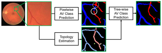
Figure 1.
Illustration of our topology-aware retinal artery–vein (AV) classification method, where estimated vessel topology is used to perform tree-wise AV classification. Red and blue colors represent classified arteries and veins, respectively. Different colors in the estimated topology map represent separate sub-trees. Tree-wise AV classification is used to correct the pixelwise classification errors on thin vessels, highlighted by white circles, which may occur due to their indistinct appearances.
Several graph-theoretic approaches have been developed with similar objectives, which are to make use of the underlying vessel topology for improved AV classification [9,10,11]. In [9], different rule-based algorithms are applied for each node degree to classify the node type into connecting, bifurcation, crossing, and meeting points in a graph generated from the vessel segmentation. Afterward, starting from the edge farthest from the optic disc center, each edge is iteratively labeled based on the estimated type of the connected node. Meanwhile, Estrada et al. [10] use a global likelihood model to attain the most plausible label set given a semi-automatically extracted planar vessel graph. Recently, the concept of dominant set clustering is adopted and gradually applied twice for topology estimation and AV classification in [11]. Compared to the previous works, different heuristic rules for different node degrees [9], complex optimization schemes for the solution [10], and manual feature design for classification [9,10,11] are not required in the proposed method.
In our work, topology estimation is formulated as iterative vascular connectivity prediction, which is specifically implemented as deep-learning-based pairwise classification between vessel pixels across a junction. We note that we will use the junction as a term including bifurcation and crossing in this work. In the proposed network, the connectivity classification is efficiently carried out for any pixel pair on top of vascular shape features, which are learned using thickness/orientation supervisions generated from segmentation ground-truths (GTs). This design is based on the observation that: (1) Shape is more distinct than appearance on thin vessels, (2) thickness/orientation changes at a bifurcation show specific patterns that can be learned [14], and (3) thickness/orientation are not abruptly changed on the same vessel at a crossing.
The main contributions of our work are as follows. (1) Our work is the first, to the best of our knowledge, to cast vessel topology estimation as an iterative connectivity prediction, which is implemented as deep-learning-based pairwise classification. (2) For both efficiency and effectiveness in the testing time, the connectivity prediction is carried out on top of convolutional feature maps learned using vascular shape supervisions, which enables a batch processing of a bunch of pixel pairs. (3) To evaluate the proposed method on the public DRIVE dataset, topology GTs are acquired for the set, and it will be made publicly available for the community (https://github.com/syshin1014/VCP).
We demonstrate the effectiveness of the proposed method by conducting comparative studies on two retinal image datasets.
2. Methods
Figure 2 depicts the test time block diagram of the proposed method, which is composed of four sequential phases: (1) pixelwise prediction on the optic disc and vessel, (2) vessel graph construction, (3) vessel topology estimation, and (4) final AV classification. An initial planar vessel graph is constructed from the pixelwise AV classification result. Then, the graph is re-structured as multiple sub-trees based on predicted vascular connectivities between vessel segments at each junction. Finally, each tree is classified as an artery or vein in whole via a voting scheme. Each phase will be detailed in the following sections.
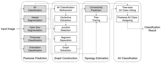
Figure 2.
Block diagram of the proposed method for AV classification at test time. Pixelwise prediction on the optic disc and vessel, graph construction, topology estimation, and the final AV classification are sequentially performed. Each block is also composed of several parallel or sequential steps. The arrows denote information flow. Gray-color boxes represent steps where the trained networks are involved. The thickness/orientation classifications are auxiliary tasks for the connectivity classification, and their relationship is not represented here. Please refer to the corresponding sections for details.
2.1. Pixelwise Prediction on the Optic Disc and Vessel
With each specialized role in the overall framework for improved AV classification, we conduct optic disc segmentation, binary vessel segmentation, and thickness/orientation classification, as well as AV classification, using CNNs.
2.1.1. Optic Disc Segmentation
The optic disc is the entry point of vessels, and it is therefore crowded with tangled vessels. Since estimating the vessel topology for such a region is nearly impossible, we perform optic disc segmentation to exclude that region from the subsequent procedures.
2.1.2. Vessel Segmentation and AV Classification
We conduct binary vessel segmentation alongside AV classification. Although this may seem to be redundant, we found that training both tasks in a multi-task manner is effective in terms of improving the accuracy. Furthermore, we use the binary vessel segmentation to filter out false positives in the AV classification, since it performs better than AV classification on separating vessels from the background.
2.1.3. Vascular Thickness/Orientation Classification
GT labels for these can be generated from vessel segmentation GTs. As for the thickness, a distance transform is firstly applied to the segmentation GT for computing distances to the closest vessel boundary. Then, for each pixel on vessel centerlines, the distance value is doubled and recorded. As for the orientation, vessel centerlines are partitioned into segments of a certain length (five pixels here). The angle between the x-axis and the straight line connecting the end points of each segment is computed in a range of . The computed thickness/orientation values are respectively assigned to nearby vessel pixels using Voronoi tessellation. The computed thickness/orientation values are finally quantized to train classification models.
2.1.4. Network Architecture
We adopt the network in [7], which is based on the VGG-16 network [15], as our base network. In this network, the final output is inferred from concatenated multi-scale features of the VGG-16. Before the concatenation, feature maps are resized to have identical spatial resolutions. A more complex network called U-Net [16] showed no differences in the performance.
For all five aforementioned tasks, we use pixelwise softmax cross-entropy losses. The loss for optic disc segmentation, which is easily generalizable for other tasks, is defined as:
where and are the one-hot encoded GT label and the class prediction for pixel , respectively. The weights for class-balancing are omitted for brevity. X is a set of pixels involved in the training, which is the set of all pixels in an image unless otherwise noted. We experimentally confine X to centerline pixels in thickness model training. This coincides with an impression that the thickness might be more well defined at on-centerline pixels than at off-centerline pixels.
Figure 3 visualizes three network architectures used for topology-aware AV classification. The first network is for optic disc segmentation and is the base network itself in terms of the architecture (Figure 3a). The second is a multi-task network for binary vessel segmentation and AV classification, which is composed of one shared encoder and two separate decoders for each task (Figure 3b). These two correlated tasks are grouped for both efficiency and effectiveness. The loss function for training this network is defined as the weighted summation of two losses and , and is given by:
where and are the weights for each task.
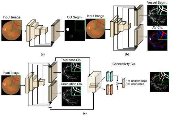
Figure 3.
Three networks for topology-aware AV classification. For each network, an input image and the corresponding ground-truth (GT) image for training are presented. For all three component networks, we adopt the network of [7] as the backbone network. (a) Network for optic disc segmentation (OD segm.). (b) Multi-task network for binary vessel segmentation and AV classification (cls.), which is composed of one shared encoder and two separate decoders for each task. (c) Network for vascular connectivity classification, including multi-task auxiliary outputs for thickness/orientation classifications. To ensure the symmetry of this pairwise classification, a Hadamard product symbolized by ⊙ is used on the 256-dim outputs of a fully connected layer applied on the concatenated thickness/orientation features. This is followed by the final fully connected inference layer. The connectivity GT label for training is decided from the rightmost topology GT. Note that different intensity values in the thickness/orientation GTs represent different classes. Different colors in the topology GT represent separate sub-trees. Further details regarding the network can be found in Section 3.2.
The third is another multi-task network for thickness/orientation classification (Figure 3c). While the vessel segmentation and AV classification themselves are desired outputs from the second network, thickness/orientation classifications in this network are trained as auxiliary tasks to learn desired features, which will be input for the vascular connectivity classification. The connectivity classification is implemented using fully connected (fc) layers on top of the concatenation of the penultimate layer features of the auxiliary tasks. For any two pixels that are respectively on different vessel segments joining at a junction, features extracted at their image coordinates are fed into the fc layers. One of the desired properties for the pairwise classification is to satisfy symmetry, which means that the output is the same regardless of the input order. To accomplish this, we use a Hadamard product (element-wise product) of two feature vectors to make a single vector for the final inference [17], as shown in Figure 3c. We again use a softmax cross-entropy loss for the connectivity classification, which is termed . The connectivity GT label for training is decided from topology GTs exemplified in Figure 3c. The loss function for training the connectivity classification network is then defined as the weighted summation of the two auxiliary task losses, and , and the connectivity classification loss , which is given by:
where , , and are the weights for each task.
2.2. Graph Construction
In the methods of [9,11], an initial graph constructed from the vessel segmentation result is modified using heuristic methods to correct typical error types like a false link between parallel vessels. We can see from Figure 4 that using the vessel segmentation result for the graph construction is inherently prone to making false links between arteries and veins. Therefore, we construct a graph from the pixelwise AV classification result instead.
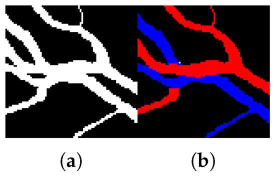
Figure 4.
An example of (a) binary vessel segmentation and (b) AV classification on arteries (red) and veins (blue) that are parallel and touching each other.
Before the graph construction, the AV classification result is simply refined by multiplying with the binary vessel segmentation. It reduces false positives, since the vessel segmentation is better in separating vessels from background. We also remove vessels within the segmented optic disc, as mentioned in Section 2.1.1. Then, the following are performed on the refined AV classification map: (1) centerline extraction by morphological thinning for arteries and veins, (2) logical OR operation on the two centerline maps of (1) for generating a single map, (3) junction detection by locating intersection points on the centerlines, and (4) vessel segment separation by removing the detected junction points.
An initial graph is constructed as an undirected graph. is a set of vertices and is defined by setting each vessel segment as a vertex. Thus, the number of vertices, N, is equal to the number of vessel segments. We will call as the j-th vertex or the j-th segment according to the context. Since each segment is composed of many pixels, we denote the j-th segment as a set , where is the number of centerline pixels composing the j-th segment. E is a set of edges, and an edge is constructed for every possible segment pair at every junction. For a junction where four segments join, we have numbers of edges. All of those pairs are considered in the connectivity prediction.
2.3. Vessel Topology Estimation
2.3.1. Vascular Connectivity Prediction
The output of the connectivity classification network in Figure 3c is a probability, between two vessel pixels, of being physically connected. More specifically, the probability is defined between a pixel on the j-th segment and another pixel on the k-th segment. W represents the learned network parameters. We note that the connectivity classification is carried on top of convolutional vascular shape features, which enables a batch processing given a bunch of pixel pairs.
The connectivity probability between the j-th and the k-th vessel segments is then computed by averaging the probabilities of pixel pairs, and is defined by:
where is a set of all possible pixel pairs within a certain distance range from the junction. By repeating this computation for all segment pairs defined in E, we finally acquire a set of the connectivity probabilities of all segment pairs, which is .
2.3.2. Tree Tracing via Connectivity Prediction
Algorithm 1 shows the pseudocode of our simple and intuitive algorithm for tree tracing. While the farthest part from the optic disc center is firstly labeled in [9], we start the tracing from the thinnest terminal segment (segment with a terminal pixel). Since vessels become thinner when being spread out, we believe that the criterion based on the thickness is more appropriate to choose the stable start point for tracing, which is located in a uncrowded region. The thickness of the j-th segment is defined by:
where is the predicted class probability vector for the thickness on pixel , which can be acquired as a side output from the connectivity classification network in Figure 3c.
| Algorithm 1: Tree tracing via connectivity prediction. |
 |
In Algorithm 1, starting from the terminal pixel of a selected terminal segment, tracking along the segment and tree label propagation to connected segments are iteratively performed until all segments are tracked. In consequence, all vessel segments are assigned respective tree labels by which the initial graph is divided into multiple trees.
2.4. Final AV Classification
Each separate tree is then classified as an artery or vein using a voting scheme where the probability vectors of all constituent centerline pixels are averaged. To prevent false AV classification as a result of erroneous tree construction, we also compute the segment-wise probability again using a voting scheme without considering the tree estimation result. If the segment-wise probability of being an artery/vein is higher than 0.8, the vessel segment is re-assigned a label as an artery/vein.
To facilitate a direct comparison with the pixelwise AV classification results, we need to remake those from the centerline classification results. Each pixel on the binary vessel segmentation is assigned an AV class according to the distances to the nearest artery and vein centerline pixels. Since the vessels within the segmented optic disc are not considered in the graph construction, the prediction of the region is copied directly from the pixelwise prediction.
3. Results and Discussion
3.1. Dataset
We experimented on two retinal image datasets, namely DRIVE [18] and IOSTAR [19], which were acquired using a fundus camera and a scanning laser ophthalmoscope (SLO) camera, respectively. For training the networks in Figure 3, GTs for optic disc segmentation, AV classification, and topology estimation are required, along with those for binary vessel segmentation.
The DRIVE dataset, which consists of 40 images, was divided into the first and last half for testing and training, respectively. Two AV GT datasets, called AV-DRIVE [20] and CT-DRIVE [9], are publicly available for the DRIVE dataset. In the AV-DRIVE dataset, all vessel pixels were marked as arteries or veins for all training and testing images. On the other hand, vessel centerline pixels were labeled only for the test set images in the CT-DRIVE dataset. We evaluated a model trained with the AV-DRIVE training set on the CT-DRIVE test set. The GTs for optic disc segmentation and topology were manually achieved by the first and second authors, who both have more than five years of experience in developing technology for vessel analysis. Furthermore, the achieved GT was inspected and verified by a board-certified ophthalmologist to ensure its validity.
For the IOSTAR dataset, we used available AV classification and topology GTs introduced respectively in [11,19], and acquired our own GTs for optic disc segmentation. Since the topology GTs were made for the downsampled version of the images, we accordingly transformed the other GTs to coincide with the size. For 18 images that had all the types of GTs, the first and last halves were used for training and testing, respectively.
3.2. Evaluation Details
In order to train the auxiliary tasks of the connectivity classification network as classification tasks, we quantized the calculated thickness and orientation values. For the thickness, we made five classes using quantization boundaries of [1.5, 3, 5, 7]. For the orientation task, every pixel was classified into one of seven classes, including six classes evenly dividing the range of and one background class.
To cope with the increased problem complexity compared to the binary vessel segmentation, which was an original task solved in [7], we changed the number of channels of multi-scale features from 16 to 32 for the thickness/orientation classification. We used two fc layers, one layer before and after the Hadamard product, for the connectivity classification, and the number of units of the first fc layer was set to 256.
Since the tasks of AV and thickness/orientation classifications are about the type and shape characteristics of vessels, we trained those networks using a pretrained network trained for the vessel segmentation. When training the multi-task network for binary vessel segmentation and AV classification, we used 1, 10, and for , , and the learning rate on the DRIVE set, and 0.01, 1, and on the IOSTAR set. As for the training of the connectivity classification network, we use a two-step training scheme. We firstly trained the network only using the auxiliary tasks, and then trained the whole network. Thus, we used in the first step. In the second step, we used 100/10 for and / for the learning rate on the DRIVE/IOSTAR sets, respectively. and were always fixed to 1. We used the learning rate value of for the optic disc segmentation network. We used an Adam optimizer [21] to train all the networks.
The types of data augmentation used for training each network are summarized in Table 1. A local contrast enhancement using a high-pass filter was applied to an input image for all the networks in the DRIVE set, while it was applied only for the connectivity classification network in the IOSTAR set. We used a threshold of 0.5 for the connectivity probability for all datasets.

Table 1.
Data augmentation used for training the networks, each of which is for (a) optic disc segmentation, (b) binary vessel segmentation and AV classification, and (c) vascular connectivity classification. Horizontal flipping, rotation (rot.), scaling, elastic deformation, cropping, random brightness, and contrast adjustment are selectively applied according to the task and the dataset.
To evaluate the proposed AV classification method, we adopted the three metrics—sensitivity, specificity, and accuracy—used in [10]. The sensitivity and specificity are defined by:
where , , , and are the true positives, true negatives, false positives, and false negatives, respectively. Here, arteries and veins are regarded as positives and negatives, respectively. The accuracy is defined as the mean of the sensitivity and the specificity.
3.3. Comparison with Previous Methods
3.3.1. Quantitative Evaluation
Table 2 compares our method with the previous methods on the CT-DRIVE dataset. It is clear that our method outperforms the compared methods, except that of [10]. We note that the proposed method operates in a fully automatic manner, while the method in [10] assumes a semi-automatically extracted input graph. In addition, it is much more time-consuming than the proposed method due to its complex optimization step for the solution.
Table 2.
Performances of different AV classification methods on the CT-DRIVE dataset. Accuracy (Acc), sensitivity (Se), specificity (Sp), and average per-image computation time are presented.
Table 3 shows the performances separately for thick and thin vessels on the IOSTAR dataset. Thick vessels are defined as being wider than three pixels. The corresponding results of the pixelwise prediction and using a segment-wise voting are also presented for comparison. We can see that: (1) The proposed tree-wise prediction method based on estimated tree structure improves the performance both on thick and thin vessels, which results in an overall accuracy improvement, and (2) the performance is also higher than that of using a segment-wise voting scheme, which means that the use of the underlying vessel topology is effective for better AV classification. We also report the area under the receiver operating characteristic curve of the vascular connectivity classification. The values were calculated as 91.1% and 82.7% for the CT-DRIVE and IOSTAR sets, respectively.
Table 3.
Performances of the proposed AV classification method on thick and thin vessels for the IOSTAR dataset. The boundary for the thick and thin vessels is a width of three pixels. The performances of the pixelwise prediction and using a segment-wise voting are also presented for comparison.
3.3.2. Qualitative Evaluation
Figure 5 and Figure 6 show the qualitative results for the CT-DRIVE and IOSTAR datasets, respectively. We can see that: (1) The tree-wise results based on the estimated vessel topology clearly show the improvement on thin or terminal vessels compared to the pixelwise prediction results, and (2) the proposed method gives more spatially consistent results along the vessel structure. The abrupt class changes either on each segment or between connected segments are suppressed in the results by the proposed method.
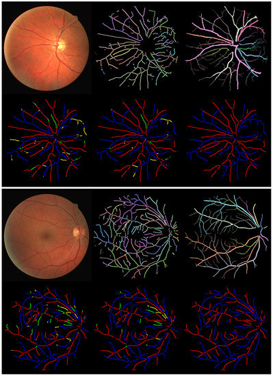
Figure 5.
Two example results from the CT-DRIVE dataset. The six images for a single case are, in row-major order beginning from the top-left, the original input image, estimated topology of the proposed method, GT annotation of the topology, pixelwise AV classification result, tree-wise classification result of the proposed method, and AV GT annotation. Different colors in the topology GT represent separate trees. In each result, correctly classified arteries and veins are marked as red and blue, respectively. Centerlines incorrectly labeled as veins are in green, while those incorrectly labeled as arteries are in yellow.
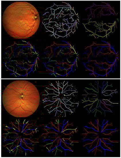
Figure 6.
Two example results from the IOSTAR dataset. The six images for a single case are, in row-major order beginning from the top-left, the original input image, estimated topology of the proposed method, GT annotation of the topology, pixelwise AV classification result, tree-wise classification result of the proposed method, and AV GT annotation. Different colors in the topology GT represent separate trees. In each result, correctly classified arteries and veins are marked as red and blue, respectively. Pixels incorrectly labeled as veins are in green, while those incorrectly labeled as arteries are in yellow.
4. Conclusions
We have proposed a novel framework for AV classification based on vessel topology estimation, which is implemented as iterative vascular connectivity prediction. The experimental results on two retinal image datasets proved the effectiveness of the proposed method. The prevention of abrupt class flipping on the same vessel tree, which can be easily observed in the pixelwise prediction result, results in more spatially consistent classification results and a special improvement for thin vessels. In the current method, the topology estimation is performed by a series of independent connectivity classifications from the end of the vessel, which is computationally efficient, but may produce an error when multiple junctions exist in a small region. For future works, we plan to extend the proposed method to utilize a longer tracing history to better classify the vascular connectivity.
Author Contributions
Conceptualization, S.Y.S., S.L., I.D.Y., and K.M.L.; methodology, S.Y.S. and S.L.; software, S.Y.S.; validation, S.Y.S., S.L., I.D.Y., and K.M.L.; formal analysis, S.Y.S.; investigation, S.Y.S. and S.L.; resources, S.L., I.D.Y., and K.M.L.; data curation, S.Y.S.; writing—original draft preparation, S.Y.S.; writing—review and editing, S.L., I.D.Y., and K.M.L.; visualization, S.Y.S. and S.L.; supervision, S.L., I.D.Y., and K.M.L.; project administration, I.D.Y. and K.M.L.; funding acquisition, S.L., I.D.Y., and K.M.L. All authors have read and agreed to the published version of the manuscript.
Funding
This work was supported by the National Research Foundation of Korea (NRF) grants funded by the Korean government (MSIT) (No. 2017R1A2B2011862, 2019R1A2C1085113, and 2020R1F1A1051847).
Institutional Review Board Statement
Not applicable.
Informed Consent Statement
Patient consent was waived due to all data being from publicly available sources provided by the authors of the studies referenced in the manuscript [9,11,18,19,20].
Data Availability Statement
Restrictions apply to the availability of these data. All data were obtained from publicly available sources provided by the authors of the studies referenced in the manuscript [9,11,18,19,20]. Generated data in this work will be made publicly available: https://github.com/syshin1014/VCP.
Conflicts of Interest
The authors declare no conflict of interest. The funders had no role in the design of the study; in the collection, analyses, or interpretation of data; in the writing of the manuscript, or in the decision to publish the results.
References
- Rousso, L.; Sowka, J. Review of Optometry: Annual Retina Report: Recognizing Abnormal Vasculature. Available online: https://www.reviewofoptometry.com/article/recognizing-abnormal-vasculature (accessed on 30 December 2020).
- Sun, C.; Wang, J.J.; Mackey, D.A.; Wong, T.Y. Retinal Vascular Caliber: Systemic, Environmental, and Genetic Associations. Surv. Ophthalmol. 2009, 54, 74–95. [Google Scholar] [CrossRef] [PubMed]
- Lesage, S.R.; Mosley, T.H.; Wong, T.Y.; Szklo, M.; Knopman, D.; Catellier, D.J.; Cole, S.R.; Klein, R.; Coresh, J.; Coker, L.H.; et al. Retinal microvascular abnormalities and cognitive decline. Neurology 2009, 73, 862–868. [Google Scholar] [CrossRef] [PubMed]
- Wang, J.J.; Liew, G.; Klein, R.; Rochtchina, E.; Knudtson, M.D.; Klein, B.E.; Wong, T.Y.; Burlutsky, G.; Mitchell, P. Retinal vessel diameter and cardiovascular mortality: Pooled data analysis from two older populations. Eur. Heart J. 2007, 28, 1984–1992. [Google Scholar] [CrossRef] [PubMed]
- Liew, G.; Wang, J.J. Retinal vascular signs: A window to the heart? Rev. Esp. Cardiol. (Engl. Ed.) 2011, 64, 515–521. [Google Scholar] [CrossRef] [PubMed]
- Niemeijer, M.; Abràmoff, M.D.; van Ginneken, B. Fast detection of the optic disc and fovea in color fundus photographs. Med. Image Anal. 2009, 13, 859–870. [Google Scholar] [CrossRef] [PubMed]
- Maninis, K.K.; Pont-Tuset, J.; Arbeláez, P.; Van Gool, L. Deep Retinal Image Understanding. In Medical Image Computing and Computer-Assisted Intervention—MICCAI 2016; Ourselin, S., Joskowicz, L., Sabuncu, M.R., Unal, G., Wells, W., Eds.; Springer International Publishing: Cham, Switzerland, 2016; pp. 140–148. [Google Scholar]
- Shin, S.Y.; Lee, S.; Yun, I.D.; Lee, K.M. Deep vessel segmentation by learning graphical connectivity. Med. Image Anal. 2019, 58, 101556. [Google Scholar] [CrossRef] [PubMed]
- Dashtbozorg, B.; Mendonça, A.M.; Campilho, A. An Automatic Graph-Based Approach for Artery/Vein Classification in Retinal Images. IEEE Trans. Image Process. 2014, 23, 1073–1083. [Google Scholar] [CrossRef] [PubMed]
- Estrada, R.; Allingham, M.J.; Mettu, P.S.; Cousins, S.W.; Tomasi, C.; Farsiu, S. Retinal Artery-Vein Classification via Topology Estimation. IEEE Trans. Med. Imaging 2015, 34, 2518–2534. [Google Scholar] [CrossRef] [PubMed]
- Zhao, Y.; Xie, J.; Su, P.; Zheng, Y.; Liu, Y.; Cheng, J.; Liu, J. Retinal Artery and Vein Classification via Dominant Sets Clustering-Based Vascular Topology Estimation. In Medical Image Computing and Computer Assisted Intervention—MICCAI 2018; Frangi, A.F., Schnabel, J.A., Davatzikos, C., Alberola-López, C., Fichtinger, G., Eds.; Springer International Publishing: Cham, Switzerland, 2018; pp. 56–64. [Google Scholar]
- Welikala, R.; Foster, P.; Whincup, P.; Rudnicka, A.; Owen, C.; Strachan, D.; Barman, S. Automated arteriole and venule classification using deep learning for retinal images from the UK Biobank cohort. Comput. Biol. Med. 2017, 90, 23–32. [Google Scholar] [CrossRef] [PubMed]
- Niemeijer, M.; Xu, X.; Dumitrescu, A.V.; Gupta, P.; van Ginneken, B.; Folk, J.C.; Abramoff, M.D. Automated Measurement of the Arteriolar-to-Venular Width Ratio in Digital Color Fundus Photographs. IEEE Trans. Med. Imaging 2011, 30, 1941–1950. [Google Scholar] [CrossRef] [PubMed]
- Sherman, T.F. On connecting large vessels to small. The meaning of Murray’s law. J. Gen. Physiol. 1981, 78, 431–453. [Google Scholar] [CrossRef] [PubMed]
- Simonyan, K.; Zisserman, A. Very Deep Convolutional Networks for Large-Scale Image Recognition. arXiv 2014, arXiv:1409.1556. [Google Scholar]
- Ronneberger, O.; Fischer, P.; Brox, T. U-Net: Convolutional Networks for Biomedical Image Segmentation. In Medical Image Computing and Computer-Assisted Intervention—MICCAI 2015; Navab, N., Hornegger, J., Wells, W., Frangi, A., Eds.; Springer International Publishing: Cham, Switzerland, 2015; pp. 234–241. [Google Scholar]
- Atarashi, K.; Oyama, S.; Kurihara, M.; Furudo, K. A Deep Neural Network for Pairwise Classification: Enabling Feature Conjunctions and Ensuring Symmetry. In Advances in Knowledge Discovery and Data Mining; Kim, J., Shim, K., Cao, L., Lee, J.G., Lin, X., Moon, Y.S., Eds.; Springer International Publishing: Cham, Switzerland, 2017; pp. 83–95. [Google Scholar]
- Staal, J.; Abramoff, M.D.; Niemeijer, M.; Viergever, M.A.; van Ginneken, B. Ridge-based vessel segmentation in color images of the retina. IEEE Trans. Med. Imaging 2004, 23, 501–509. [Google Scholar] [CrossRef] [PubMed]
- Zhang, J.; Dashtbozorg, B.; Bekkers, E.; Pluim, J.P.W.; Duits, R.; ter Haar Romeny, B.M. Robust Retinal Vessel Segmentation via Locally Adaptive Derivative Frames in Orientation Scores. IEEE Trans. Med. Imaging 2016, 35, 2631–2644. [Google Scholar] [CrossRef] [PubMed]
- Qureshi, T.A.; Habib, M.; Hunter, A.; Al-Diri, B. A manually-labeled, artery/vein classified benchmark for the DRIVE dataset. In Proceedings of the 26th IEEE International Symposium on Computer-Based Medical Systems, Porto, Portugal, 20–22 June 2013; pp. 485–488. [Google Scholar] [CrossRef]
- Kingma, D.P.; Ba, J. Adam: A Method for Stochastic Optimization. arXiv 2014, arXiv:1412.6980. [Google Scholar]
Publisher’s Note: MDPI stays neutral with regard to jurisdictional claims in published maps and institutional affiliations. |
© 2020 by the authors. Licensee MDPI, Basel, Switzerland. This article is an open access article distributed under the terms and conditions of the Creative Commons Attribution (CC BY) license (http://creativecommons.org/licenses/by/4.0/).