Large Eddy Simulation of Film Cooling with Bulk Flow Pulsation: Comparative Study of LES and RANS

Abstract

The effects of bulk flow pulsations on film cooling in gas turbine blades were investigated by conducting large eddy simulation (LES) and Reynolds-averaged Navier–Stokes simulation (RANS). The film cooling flow fields under 32 Hz pulsation in the mainstream from a cylindrical hole inclined 35° to a flat plate at the average blowing ratio of M = 0.5 were numerically simulated. The LES results were compared to the experimental data of Seo, Lee, and Ligrani (1998) and Jung, Lee, and Ligrani (2001). The credibility of the LES results relative to the experimental data was demonstrated through a comparison of the time-averaged adiabatic film cooling effectiveness, time- and phase-averaged temperature contours, Q-criterion contours, time-averaged velocity profiles, and time- and phase-averaged U_rms profiles with the corresponding RANS results. The adiabatic film cooling effectiveness predicted using LES agreed well with the experimental data, whereas RANS highly overpredicted the centerline effectiveness. RANS could not properly predict the injectant topology change in the streamwise normal plane, but LES reproduced it properly. In the case of the injectant trajectory, which greatly influences film cooling effectiveness, RANS could not properly predict the changes in the streamwise velocity peak due to flow pulsation, but they were predicted well with LES. RANS greatly underpredicted the streamwise velocity fluctuations, which determine the mixing of main flow and injectant, whereas LES prediction was close to the experimental data.

1. Introduction

The idealized Brayton cycle indicates that the efficiency of gas turbines could be increased by increasing the turbine inlet temperature [1]. However, the blade surface temperature should be maintained below a tolerable limit to avoid excessive thermal stress on the blade. Film cooling is a widely used cooling method for turbine blades. The coolant bled from the compressor is injected onto the blade surface through small holes on the surface, and the resulting coolant film protects the surface from the hot mainstream by reducing the surface temperature.

Multiple variables affect the performance of film cooling, and they are often studied by performing numerical analysis to save cost and time. In film cooling flow fields, turbulence is generated, and it can be modeled by conducting Reynolds-averaged Navier–Stokes simulations (RANSs), large eddy simulations (LESs), or by using a hybrid approach such as detached eddy simulation. It is known that the LES approach predicts the mixing between the mainstream and the coolant better than RANS turbulence models, even though its computation time is considerably longer [2,3,4].

Multiple numerical studies have been conducted to understand the film cooling physics under a steady main flow. Walters and Leylek (2000) used RAMPANT code [5] to simulate film cooling on a flat plate [6]. They used the standard k-ε of Launder and Spalding for a 3-D unstructured mesh. They found that the model could not well predict coolant reattachment in the narrow field near the hole at high blowing ratios. In addition, the RANS results overpredicted the centerline effectiveness and showed less lateral coolant spreading on the wall. Tyagi and Acharya (2003) performed an LES for film cooling [7]. They used a dynamic mixed model as the subgrid scale model and applied the velocity profiles obtained using the RANS approach to the delivery tube inlet. Their LES results yielded better predictions of the adiabatic film cooling effectiveness than the RANS results because LES was able to predict the coherent structures generated due to film cooling. Rozati and Tafti (2007) investigated the effects of turbulence in the freestream on film cooling by conducting LES [8]. They found that LES was able to capture the counter-rotating vortex pair (CRVP) and that a fully turbulent jet decreased the film cooling effectiveness by increasing mixing with the main flow.

Na et al. (2007) showed that a ramp placed upstream of the hole increased the film cooling effectiveness by inducing interaction between the main flow and the jet further away from the wall, resulting in the formation of a weaker horseshoe vortex [9]. In their simulations, the realizable k-ε model was used. Johnson, Shyam, and Hah (2011) studied the effects of ratios of the delivery tube length to hole diameter (L/D), momentum ratio, and grid resolution on the effectiveness of adiabatic film cooling by using the realizable k-ε model [10]. They found that grid refinement around the trailing edge of the hole was effective for improving the effectiveness of film cooling at high momentum ratios. In addition, they stated that the adiabatic film cooling effectiveness decreased when the jet had high momentum and the L/D ratio was small because of higher jet lift-off.

LES does not guarantee the best CFD (Computational Fluid Dynamics) results. Wojtas, Makowski, and Orciuch (2020) predicted the course of barium sulfate precipitation in jet reactors by CFD simulations and compared the results with the experimental data [11]. They performed the simulations using both LES and RANS models, showing that the results were similar and did not differ from each other significantly even though the LES approach required high computational cost. However, according to most numerical studies on film cooling, the LES approach is superior to the RANS method in predicting film cooling performance under the steady flow condition.

However, an unsteady main flow could be induced in the flow fields of film cooling due to various reasons, such as potential flow interactions, shockwaves, passing wakes, or freestream turbulence in the combustion chamber [12]. Understanding the effects of such an unsteady main flow on film cooling performance is crucial for improving the design of turbine components. However, the experimental and numerical studies on the effects of an unsteady main flow on film cooling are scarce.

Coulthard, Volino, and Flack (2000) experimentally investigated the effects of jet pulsing on film cooling performance [13]. They showed that, at higher pulsation frequencies of coolant injection, the effectiveness of film cooling decreased. They added that the best film cooling performance was obtained at M = 0.5. Nikitopoulos and Acharya (2009) numerically studied the effect of jet pulsation on film cooling and found that the effectiveness of film cooling could be controlled and improved through jet pulsation [14]. They reported that frequency, duty cycle, and blowing ratio are the three parameters that affected the film cooling performance. Even when the instability pattern in the main flow might be extremely complex, the oscillations could be approximated in the sinusoidal form because the instability pattern would be more similar to a sinusoidal waveform compared to a simple pulse.

Among the causes of the aforementioned unsteadiness of the main flow, potential flow interaction was recognized as important, and experimental studies pertaining to the effects of bulk flow pulsation on film cooling have been published. Seo, Lee, and Ligrani (1998) discussed the effects of pulsations in the main flow on film cooling at the frequencies of 2, 16, and 32 Hz [12]. They reported that, when the pulsation frequencies were increased at the average blowing ratio of M = 0.5 and short L/D, the film cooling effectiveness decreased and the heat transfer coefficients increased. Jung, Lee, and Ligrani (2001) reported that the flow structures of film cooling have phase-averaged and time-averaged velocity profiles and Reynolds stresses at 0, 2, 16, and 32 Hz for the average blowing ratio of M = 0.5 [15]. They showed that, when the pulsation frequencies were increased, the effect of increasing the frequency on the flow structures became stronger.

In this study, numerical (LES) simulations of film cooling from a cylindrical hole on a flat plate were conducted by applying bulk flow pulsations of 32 Hz. The LES results were compared to the experimental data and the RANS results to verify the improvement offered by the LES approach relative to the RANS approach in terms of predicting film cooling performance under unsteady flow conditions. First, we checked how LES and RANS separately predict changes in film cooling performance under pulsation of the main flow. It was found which turbulence model for RANS best predicts the film cooling performance. Second, we examined how LES and RANS predict the behavior of the injectant by comparing the time-averaged and phase-averaged temperature fields with the experimental results. There have not been any studies on the behavior of the coolant by comparing the phase-averaged temperature fields obtained by experiment, LES, and RANS. The comparison is presented in this paper. Next, by comparing the flow field according to the phase, we found that certain flow structures did not appear in unsteady RANS (URANS) but did appear in LES. Finally, we compared the changes in turbulence intensity due to pulsation, followed by a discussion about the turbulence intensity characteristics by phase.

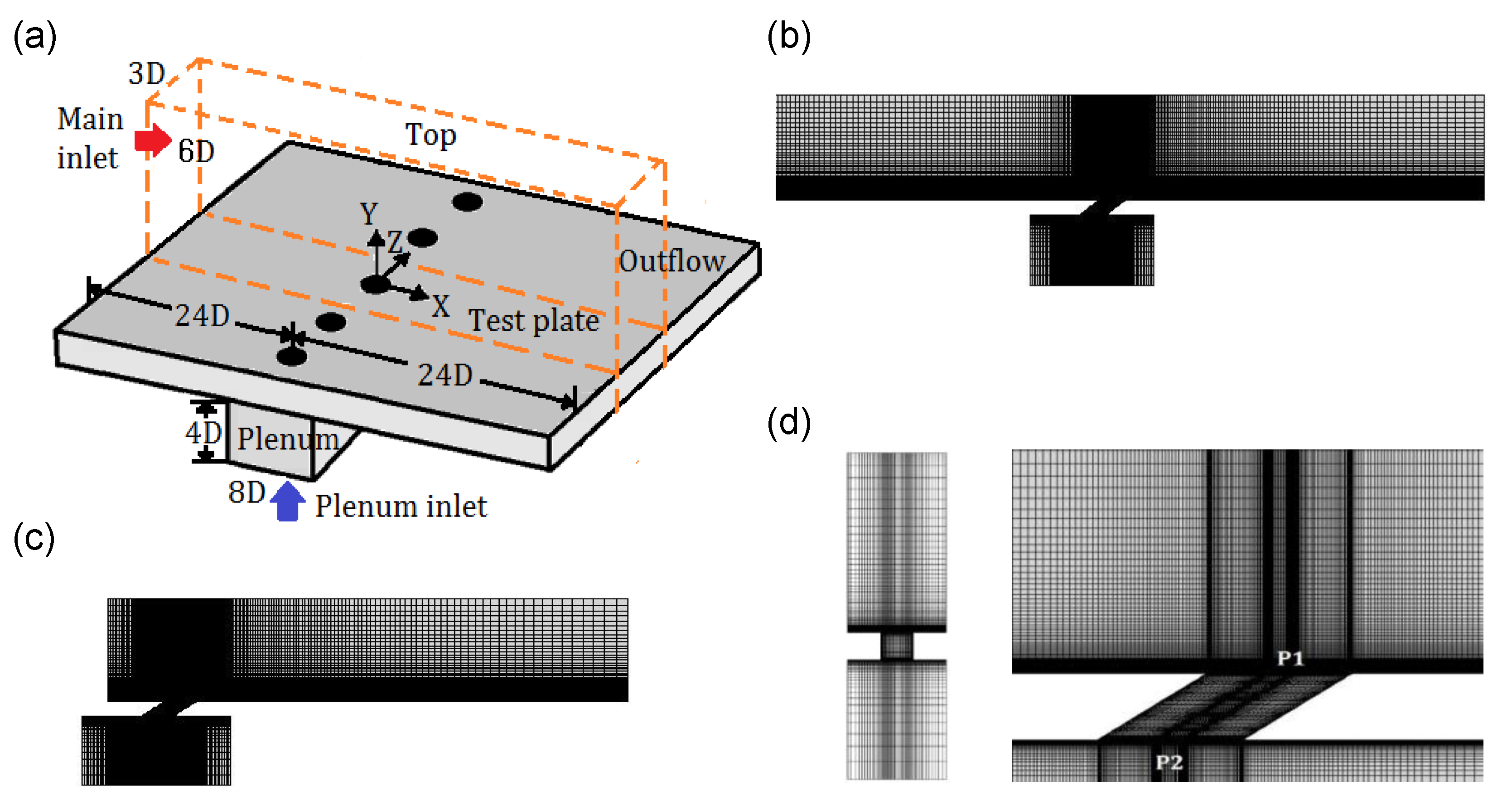
2. Geometry and Boundary Conditions

The CFD simulations were performed with a three-dimensional mesh. The orange dashed lines in Figure 1a show the computational domain. The geometry of real turbine blades is more complex than that represented by the computational domain. However, the results obtained for a flat plate could be applied to real turbine blades with some corrections [16]. The geometry was adopted from Seo, Lee, and Ligrani [12]. In their experimental facility, five cooling holes were created on the plate in a row. To reduce computation time, in the present study, the computational domain was created with a single hole by applying the periodic boundary condition to the sides of the domain.

The hole shape was cylindrical without a compound angle. The hole diameter (D) was 0.025 m, the ratio of hole length (L) to hole diameter (D) was 1.6, the ratio of pitch to hole diameter (P/D) was 3, and the injection angle (α) was 35°. The turbulence intensity of the mainstream at the main inlet was 0.2%, and the velocity of the main flow was 10 m/s. The temperatures at the main inlet and plenum inlet were 293 K and 313 K, respectively, as in the study of Seo, Lee, and Ligrani [12]. As illustrated in Figure 1a, the computational domain was extended to 24 times the hole diameter downstream and upstream of the hole center. Figure 1b shows the CFD mesh in the z = 0 plane. For the LES calculation in the steady state (0 Hz), a mesh extended to only four times the hole diameter upstream of the hole center was used to reduce computational cost (Figure 1c). The velocity profiles due to which the boundary layer thickness at the hole center was 1.02D, as stated in Seo, Lee, and Ligrani [12], and the turbulence quantities were determined using a separate flat plate mesh and applied at the main inlet of the computational mesh. Figure 1d shows the CFD mesh in the yz plane and a close-up of the mesh around the jet injection region. In total, 2.04 million hexahedral cells were used in the mesh, as shown in Figure 1b. The mesh spacing values ranged from 6 near the hole to approximately 35 at x = 24D in x⁺ units in the x-streamwise direction. The y⁺ value of the first cell above the test plate was less than 1 to ensure that the gradient of the wall-normal velocity in the viscous sublayer could be captured accurately, and there were 25 cell layers up to y⁺ = 30. The mesh spacing value in the z-spanwise direction was 20 throughout the domain in z⁺ units. If h was assumed as the hole wall-normal coordinate, the h⁺ value of the first cell was set to less than 2 to accurately capture the gradient of the wall-normal velocity in the viscous sublayer. There were 15 cell layers up to h⁺ = 40. Figure 1c illustrates a close-up of the mesh around the jet injection region. The black regions in the figure show that the fine cells were concentrated around the boundary layer and in the region where complex flow structures were induced by the interactions between the mainstream and the jet.

Table 1. Boundary conditions of the computational domain.

Surface	Boundary Condition
Main inlet	Velocity inlet
Plenum inlet	Velocity inlet
Top	Symmetry
Test plate	Adiabatic wall
Outflow	Pressure outlet
Main sides	Periodic
Sides of plenum	Wall

summarizes the boundary conditions of the domain.

As summarized in Table 1, the boundary conditions at the main inlet and plenum inlet were set as the velocity inlet. Except for the LES calculation in the steady state (0 Hz), the velocity profile at the main inlet of the mesh in Figure 1b was spatially uniform, and can be expressed as follows:

V_main = A sin(2πft) + 10 m/s.

(1)

A values, that is, the main flow velocity oscillation amplitudes, were taken from Seo, Lee, and Ligrani [12]. The values are shown in terms of frequency and Strouhal number (Sr) in

Table 2. A values in Equation (1) in terms of frequency and Strouhal number (Sr).

Frequency (Hz)	0	2	16	32
Sr	0	0.0314	0.2513	0.5027
A	0	1.82	0.57	0.44

.

The velocity profile at the plenum inlet was assumed to be spatially uniform as well. It varied with time and was expressed as follows:

V_plenum = B sin(2πft) + 0.164 m/s

(2)

where 0.164 m/s corresponds to the plenum inlet velocity in the steady state. If a sinusoidal oscillation is applied to the main inlet, an oscillation of the same frequency is generated in the coolant jet because the pressure difference between the static pressure around the delivery tube inlet (P₂) and the static pressure around the tube exit (P₁) oscillates due to oscillations in the main flow. The measurement locations of P₁ and P₂ are illustrated in Figure 1d. Therefore, in the present study, sinusoidal waveforms of the same frequency were applied to both the main inlet and the plenum inlet simultaneously. The B values for each frequency were not reported, but the P₂–P₁ variation plots for each frequency were given in Seo, Lee, and Ligrani [12]. The B values were obtained by matching the variation plots with the trial and error method. The B values, that is, the amplitudes of the plenum inlet velocity oscillation in terms of frequency and Strouhal number, are listed in

Table 3. B values in Equation (2) in terms of frequency and Strouhal number (Sr).

Frequency (Hz)	0	2	16	32
Sr	0	0.0314	0.2513	0.5027
B	0	0.04	0.05	0.16

.

3. Numerical Methods

ANSYS Fluent v.19 [17] was used to conduct the CFD calculations, and Pointwise v.18 [18] was used to generate the computational mesh. Numerical simulations were carried out using the LES and RANS approaches. The Smagorinsky–Lilly model was used as the subgrid scale model for the LES calculation. In this study, the Smagorinsky constant was 0.17, which is the default value in ANSYS Fluent. The realizable k-ε model, Reynolds stress model, and standard k-ω model were used for the RANS calculations. The time step for LES was set to 6.25 × 10⁻⁶ s, which corresponded to the time required for convection of the mainstream through the length of the hole diameter in 400 time steps [19,20]. The time step for unsteady RANS was set to 3.125 × 10⁻⁴ s, which corresponded to the period of the 32 Hz oscillation divided by 100. The solution statistics were collected for multiples of the period after the steady state was statistically achieved. For each time step, approximately 10 subiterations were performed to ensure that the data were well resolved and to reduce factorization and linearization errors [21]. Twenty cores of an Intel Xeon Gold 6148 processor were used for the computations, and the LES and RANS calculation times were approximately 2 months and less than 8 h, respectively.

3.1. Governing Equations and Turbulence Models

The fluid was assumed to be Newtonian and incompressible and to have temperature-dependent variable properties. The average blowing ratio was set to M = 0.5. The main flow velocity was 10 m/s, and the averaged jet injection velocity was 5 m/s. Both velocities were considerably less than Mach 0.3, and the effect of compressibility was negligible [22]. The continuity, momentum, and energy equations were the governing equations in the CFD simulations.

3.1.1. Unsteady RANS approach

For the 32 Hz oscillation, the unsteady RANS (URANS) approach was used because URANS can predict unsteady flow structures.

Conservation of mass (continuity equation):

$$\frac{\partial \rho }{\partial t}+\frac{\partial }{\partial x_j}\left(\rho U_j\right)=0$$

(3)

Conservation of momentum:

$$\rho \left(\frac{\partial U_i}{\partial t}+U_j\frac{\partial U_i}{\partial x_j}\right)=-\frac{dP}{d{x}_i}+\rho g{\delta }_{i3}+\frac{\partial }{\partial x_j}\left(\mu \frac{\partial U_i}{\partial x_j}-\rho \overline{u_i{u}_j}\right)$$

(4)

Conservation of energy:

$$\rho c_p\left(\frac{\partial \overline{T}}{\partial t}+U_j\frac{\partial \overline{T}}{\partial x_j}\right)=-\frac{\partial }{\partial x_j}\left(-\kappa \frac{\partial \overline{T}}{\partial x_j}+\rho c_p\overline{u_j{T}^{\prime }}\right)$$

(5)

Six Reynolds stresses, $-\rho \overline{uu}$, $-\rho \overline{uv}$, $-\rho \overline{uw}$, $-\rho \overline{vv}$, $-\rho \overline{vw}$, and $-\rho \overline{ww}$, from Equation (4) and $\overline{T^{\prime }u}$, $\overline{T^{\prime }v}$, and $\overline{T^{\prime }w}$ from Equation (5) need to be modeled [23]. A closure for these equations can be obtained using Boussinesq hypothesis, which is expressed as follows [24]:

$$-\rho \overline{{u_i}^{\prime }{u_j}^{\prime }}={\mu }_t\left(\frac{\partial u_i}{\partial x_j}+\frac{\partial u_j}{\partial x_i}-\frac{2}{3}\frac{\partial u_k}{\partial x_k}{\delta }_{ij}\right)-\frac{2}{3}\rho k{\delta }_{ij}$$

(6)

where ${\mu }_t$ represents the turbulent viscosity, and it is modeled as follows [24]:

$${\mu }_t=\frac{\rho C_{\mu }{k}^2}{\epsilon }$$

(7)

3.1.2. LES Approach

LES resolves large eddies directly, but small eddies are modeled. It filters out the eddies that are smaller than the grid spacing and resolves large eddies. This approach is reasonable because mass, energy, and momentum are mostly transported by large eddies [25]. The filtered Navier–Stokes equations for LES are as follows [17]:

$$\frac{\partial \rho }{\partial t}+ \frac{\partial }{\partial x_i}\left(\rho {\overline{u}}_i\right)=0$$

(8)

$$\frac{\partial \left(\rho \overline{u}\right)}{\partial t}+\frac{\partial }{\partial x_j}\left(\rho {\overline{u}}_i{\overline{u}}_j\right)=\frac{\partial }{\partial x_j}\left[\mu \left(\frac{\partial \overline{u_i}}{\partial x_j}+\frac{\partial \overline{u_j}}{\partial x_i}\right)-\frac{2}{3}\mu \frac{\partial \overline{u_l}}{\partial x_l}{\delta }_{ij}\right]-\frac{d\overline{p}}{dx}+\frac{\partial {\tau }_{ij}}{\partial x_j}$$

(9)

The subgrid-scale turbulent stress (${\tau }_{ij})$ is modeled using the Boussinesq hypothesis as follows [17].

$${\tau }_{ij}- \frac{1}{3}{\tau }_{kk}{\delta }_{ij}= -{\mu }_t\left(\frac{\partial \overline{u_i}}{\partial x_j}+\frac{\partial \overline{u_j}}{\partial x_i} \right)$$

(10)

4. Results and Discussion

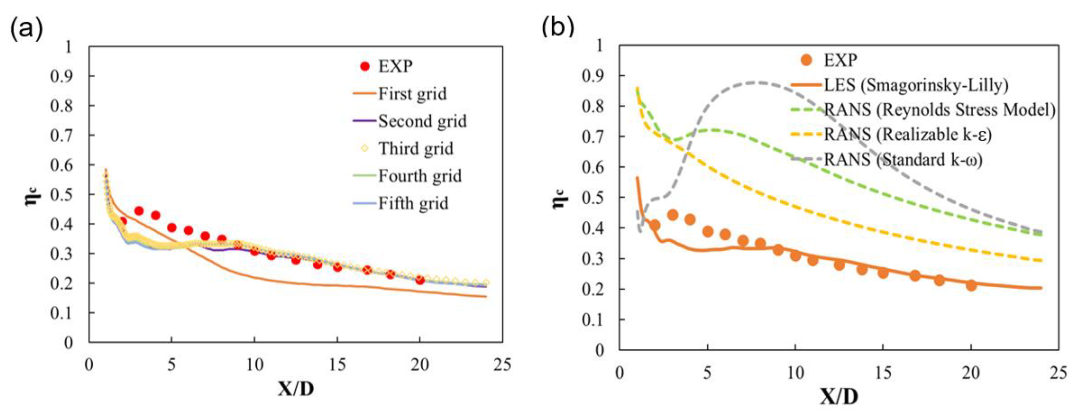
4.1. Mesh Sensitivity Test

The plots of centerline effectiveness of the mesh sensitivity test at 0 Hz for the blowing ratio M = 0.5, as obtained using the LES Smagorinsky–Lilly model, are shown in Figure 2a. Five different meshes were tested, and the specifications of each of these meshes are listed in

Table 4. Specifications of mesh arrangements in crossflow block for mesh sensitivity test.

Grid	Number of Cells in the x Direction	Number of Cells in the y Direction	Number of Cells in the z Direction	Number of Cells in the Main Block (Million)	Total Number of Cells (Million)
First	240	50	32	0.40	1.02
Second	248	60	48	0.73	1.35
Third	284	80	50	1.15	1.77
Fourth	302	94	56	1.60	2.22
Fifth	308	110	64	2.18	2.80

. The third mesh, which contained 1.77 million cells, exhibited almost the same centerline effectiveness as the two finer grids of the fourth and the fifth meshes. Therefore, the mesh with 1.77 million cells was selected to use in the CFD simulations.

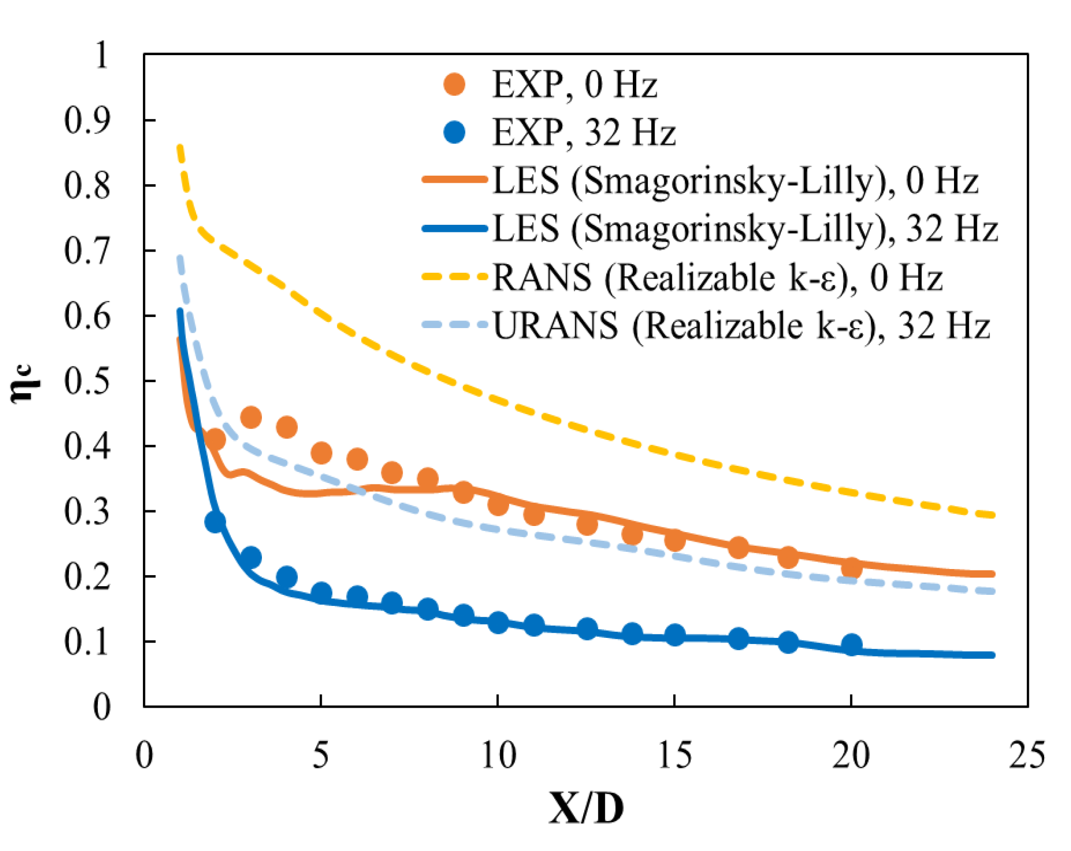
4.2. Film Cooling Effectiveness

Figure 2b illustrates that several RANS models overpredicted the centerline effectiveness in the steady state, and results of the realizable k-ε model differed the least from the experimental data. Even the Reynolds stress model, which solves more equations to reflect the anisotropy of turbulence, more severely overpredicted the centerline effectiveness than the realizable k-ε model after x/D = 5. The results of the k-ω model differed the most from the experimental results among the compared turbulence models. Based on these results, the realizable k-ε model was adopted for the unsteady RANS, in which pulsation was applied to the main flow.

It has been reported that the film cooling efficiency generally decreases when there is pulsation in the bulk flow. In particular, it has been reported that the film cooling efficiency decreases by about half when the pulsation frequency and blowing ratio are 32 Hz and 0.5, respectively [12,15,26], as observed in this study as well. As illustrated in Figure 3, both LES and URANS reproduced the decrease in film cooling efficiency upon the application of pulsation, although the RANS realizable k-ε model overpredicted the centerline effectiveness. According to the figure, the RANS model overpredicted the centerline effectiveness by approximately 57% for 0 Hz and by approximately 105% for 32 Hz, whereas the centerline effectiveness obtained in LES differed by only about 5% relative to the experimental data.

When the 32 Hz pulsation is applied, the amplitude of the pressure difference between P₁ and P₂ increased because of large phase shifts between them [12]. Then, the amplitude of the coolant velocity oscillation increased, and more jet lift-off was generated periodically, resulting in less effective film cooling. At 32 Hz, the computed cooling effectiveness of the centerline film was more accurate than that at 0 Hz because the jet lift-off effect was considerably stronger than the other vortex effects, such as horseshoe vortex or CRVP, which are detrimental to the film cooling effectiveness. Moreover, LES yielded a good prediction of jet lift-off. As shown in Figure 3, as the main flow passed downstream, the centerline effectiveness decreased, regardless of the frequency, because of the generation of the turbulence and mixing between the main flow and the jet.

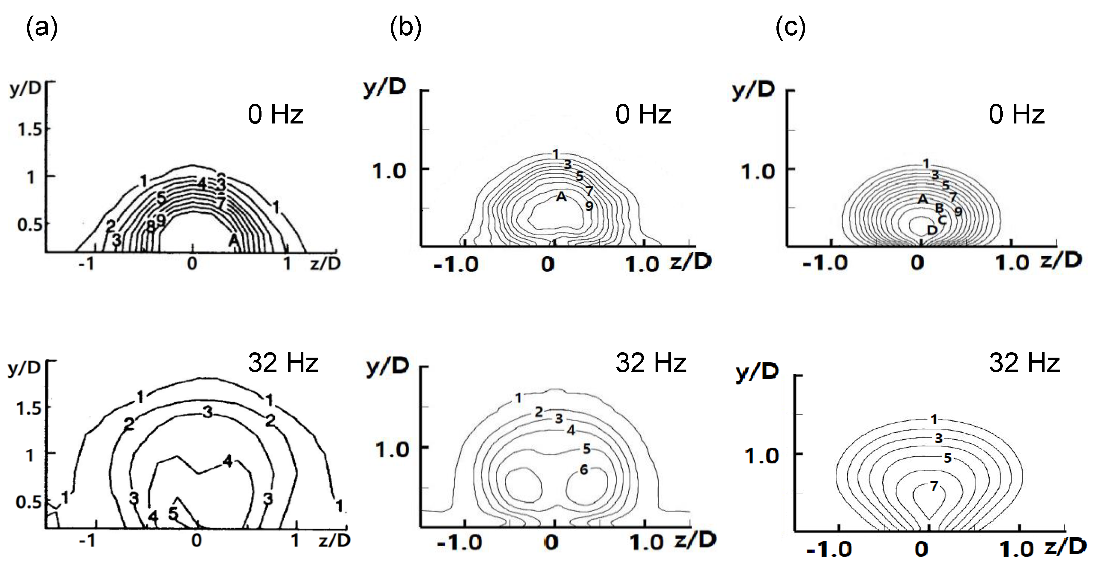
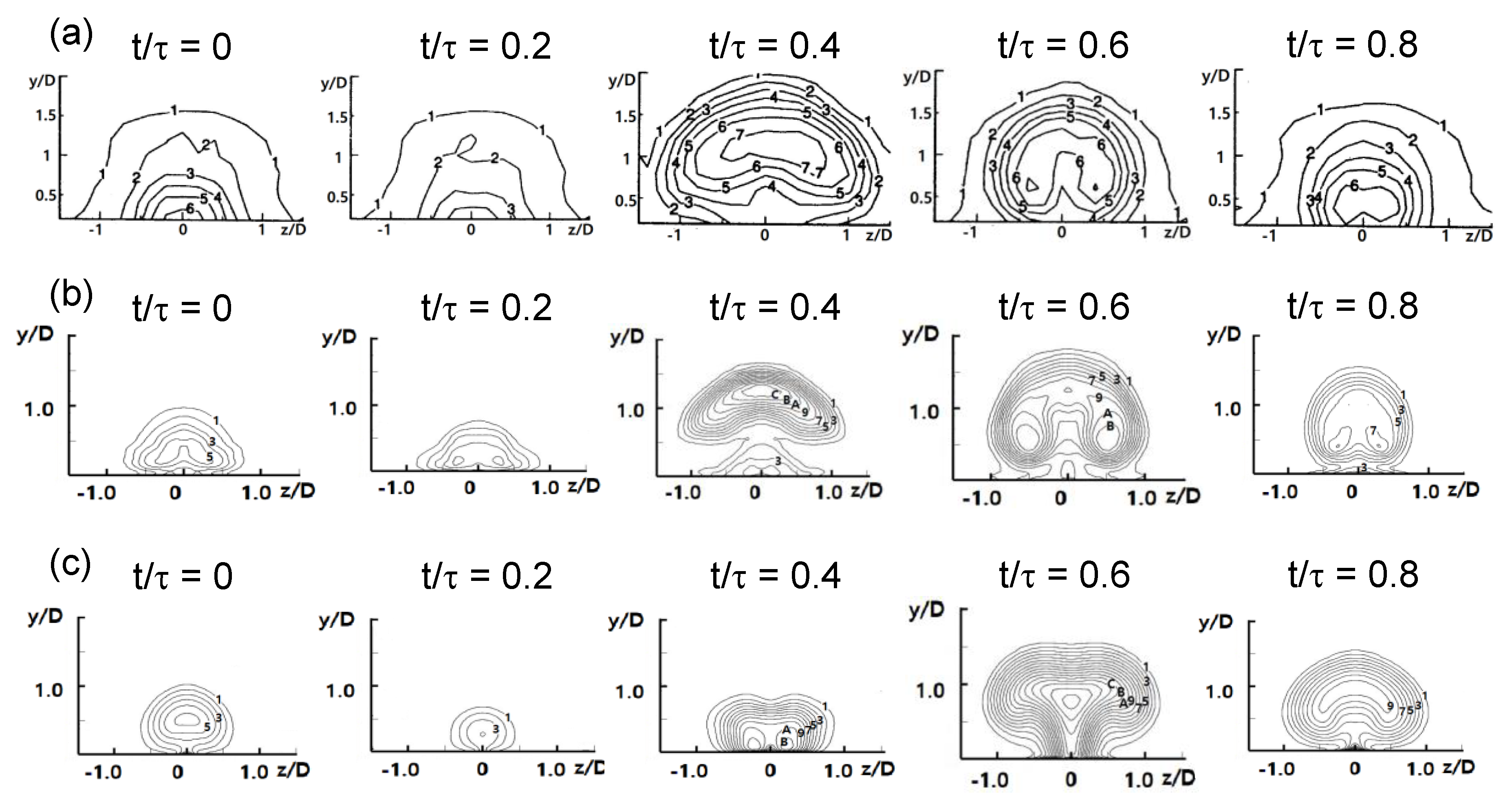
4.3. Dimensionless Temperature Contours at x/D = 5

The overprediction of the centerline film cooling effectiveness by RANS was attributed to the lower level of mixing predicted between the main flow and the jet compared to the experimental data. Figure 4 illustrates the time-averaged dimensionless temperature contours at x/D = 5 obtained experimentally [12], as well as by means of LES and RANS. In Figure 4c, the RANS results indicate that the region around the jet core barely mixes with the main flow, and the dimensionless temperature around point 0 representing the centerline is higher than the experimental results. This explains why the adiabatic centerline effectiveness was overpredicted by the RANS approach. In contrast, in Figure 4b, the dimensionless temperature of the core part obtained by LES is lower than that obtained in RANS, indicating greater mixing with the main flow. However, the mixing intensity in the LES contour is still lower than the experimental result.

Figure 5 illustrates the phase-averaged dimensionless temperature contours at x/D = 5 obtained experimentally [12], as well as by means of LES and RANS, under 32 Hz pulsation. The phase-averaged dimensionless temperature contours shown in Figure 5b were obtained by averaging 50 instantaneous LES contours to achieve bilateral symmetry. The change in the distributions was attributed to periodic changes in the blowing ratio, as given by Equation (2). The dimensionless temperature contours obtained by RANS were different from the experimental results, whereas the LES contours were quite similar to the experimental contours because the jet lift-off and various other vortexes, such as CRVP, generated due to jet injection were considerably better predicted by LES than RANS. At t/τ = 0.4, the lift-off of the injectant observed in the experiment was reproduced by LES but was not predicted by RANS. At t/τ = 0.6, a kidney-shaped temperature distribution was observed by the CRVP in the experiment. In LES, the kidney-shaped temperature distribution similar to that in the experiment was observed, but in RANS, a temperature peak occurred at z/D = 0.

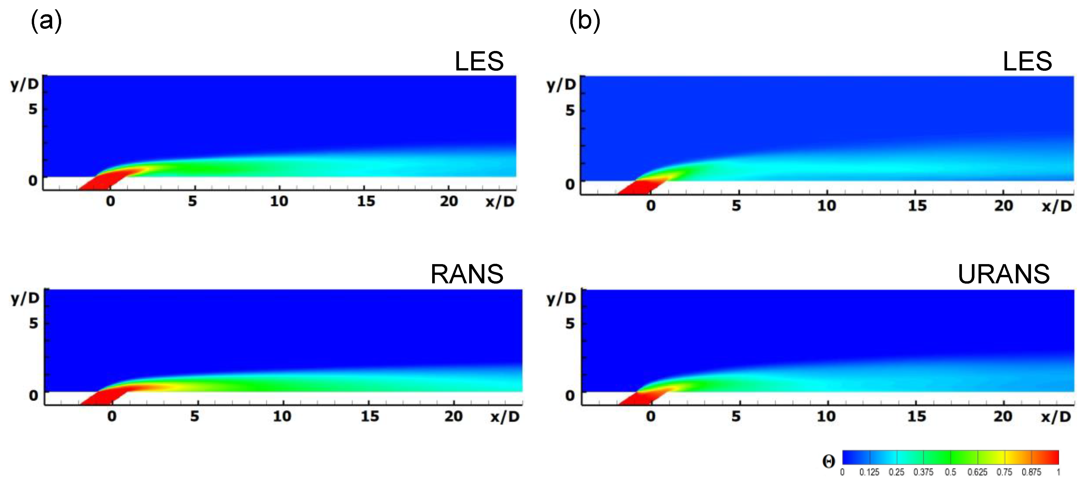
4.4. Dimensionless Temperature Contours at y/D = 0 and z/D = 0

Figure 6 shows the time-averaged film cooling effectiveness contours on the test plate obtained experimentally [26], as well as by means of LES and RANS. The experimental contours were measured for L/D = 4, having higher film cooling effectiveness than LES results for L/D = 1.6. However, they are included in Figure 6 for reference. In the case of 0 Hz, in the region where x/D is less than 3, the experimental and LES results differ because of the L/D effect, but they show similar distributions downstream. At 32 Hz, the effect of L/D decreases, and the experimental and LES results have similar distributions. The RANS result predicted less mixing with the main flow than the experimental result, so the film cooling efficiency was higher at the centerline than that in the experiment, and the film cooling efficiency was lower between the holes.

Figure 7 illustrates the time-averaged dimensionless temperature contours obtained by LES and RANS on the z = 0 plane. A comparison of the LES and RANS temperature fields in the absence of pulsation (Figure 7a) shows that, in the RANS result, the region with high dimensionless temperature (red in the contour) is longer along the surface than that in the LES result. The overprediction of the centerline film cooling effectiveness by RANS in Figure 2b can be confirmed from the time-averaged temperature contours shown in Figure 7a. Under the application of 32 Hz (Figure 7b), mixing with the main flow occurs in both the LES and the RANS results, and the red-colored region remains within the hole. In the case of LES, injectant lift-off is clearly shown compared to that in RANS, so a blue contour area can be seen near the wall after x/D = 5.

Figure 8 shows the dimensionless temperature fields obtained by means of LES and URANS at y/D = 0 and z/D = 0 for each phase with pulsation of the main flow. The figure shows periodic jet lift-off and periodic formation of large coolant vortices. As can be seen in the contours for z/D = 0, the locations of the large coolant vortices obtained using LES and URANS are similar to each other. However, the jet shear layer vortices, which are generated due to shear between the main flow and the coolant jet [27], are present within the gray circle in the LES contour at z/D = 0 in Figure 8a, whereas these vortices are absent in the URANS contours at z/D = 0. The LES contours at y/D = 0 show a wider coolant spread along the spanwise z-direction than the URANS contours. Moreover, the horseshoe vortex is clearly visible in the LES contours at y/D = 0, as in Figure 8a, whereas this vortex is not clearly visible in the URANS contours at z/D = 0, as in Figure 8b.

4.5. Q-criterion Contours at z/D = 5 and y/D = 0

In the Q-criterion, Q is defined as the difference between the magnitude of the rotation rate and the strain rate, and it represents the dominance of the rotation rate compared to the strain rate [28,29]. Figure 9a,b shows the instantaneous Q-criterion contours with iso-surfaces of levels 1000 and 500, colored with vorticity ω_z for the 32 Hz pulsation, and obtained with LES and URANS, respectively. The Q-criterion contours are colored with y-vorticity in each phase. Compared to the Q-criterion contours predicted using URANS, those predicted by LES indicate that LES can predict more complex vortex structures, including CRVP, hairpin, jet shear layer, and horseshoe vortices. URANS predicted only simple vortex structures, such as the horseshoe vortex and the hairpin vortex, as shown in Figure 9b. In the Q contour obtained using LES, complex vortical structures continuously exist under the injectant, but in the URANS result, they appear partially under the hairpin vortices.

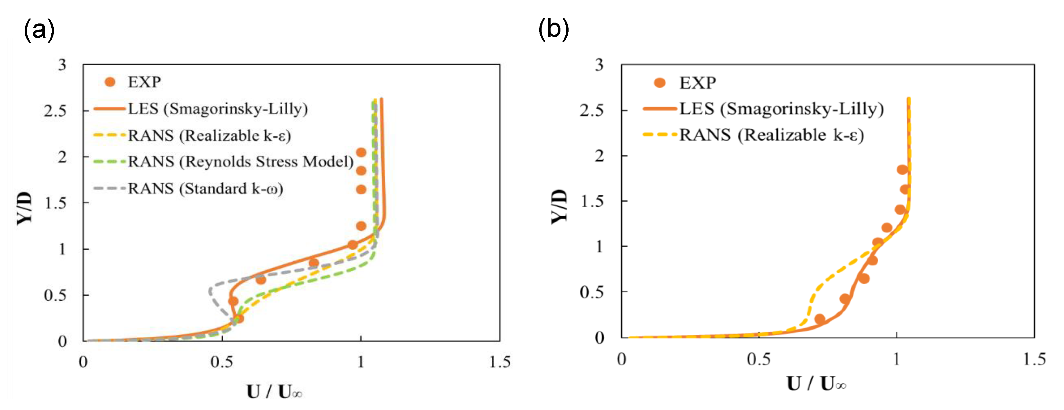
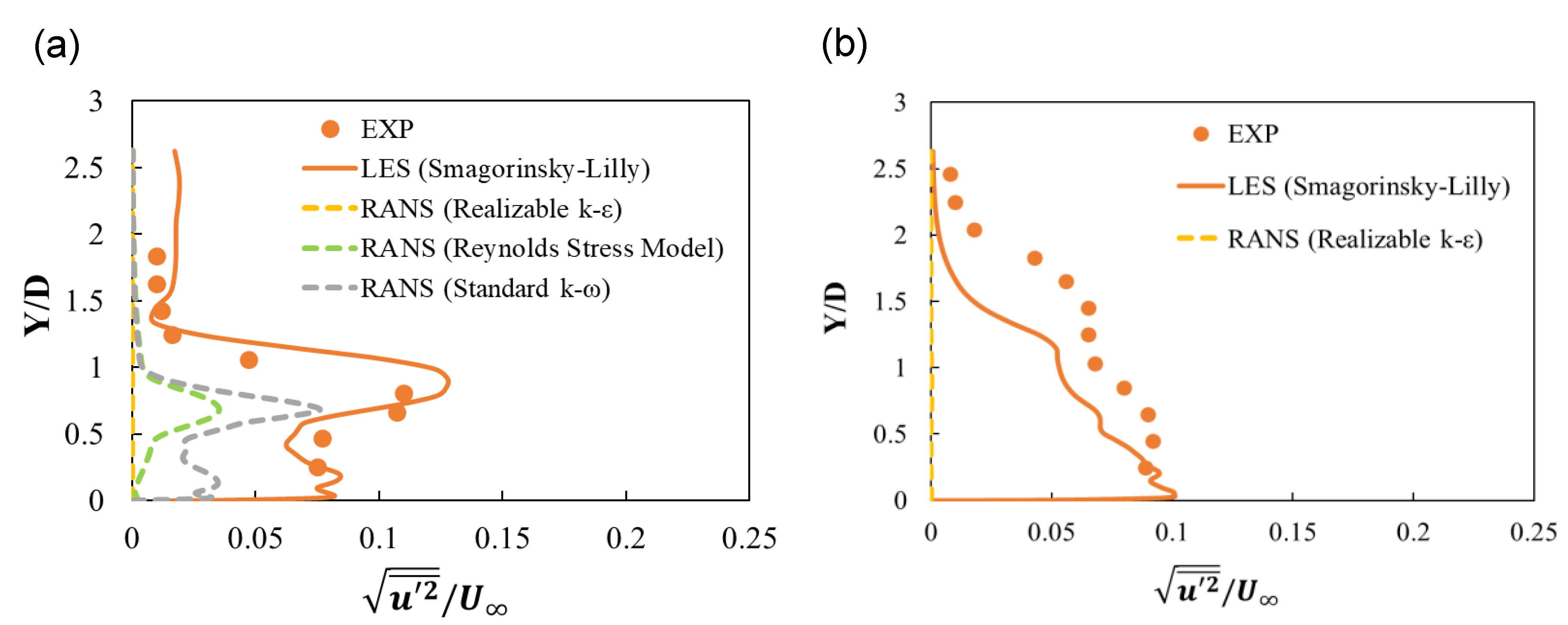
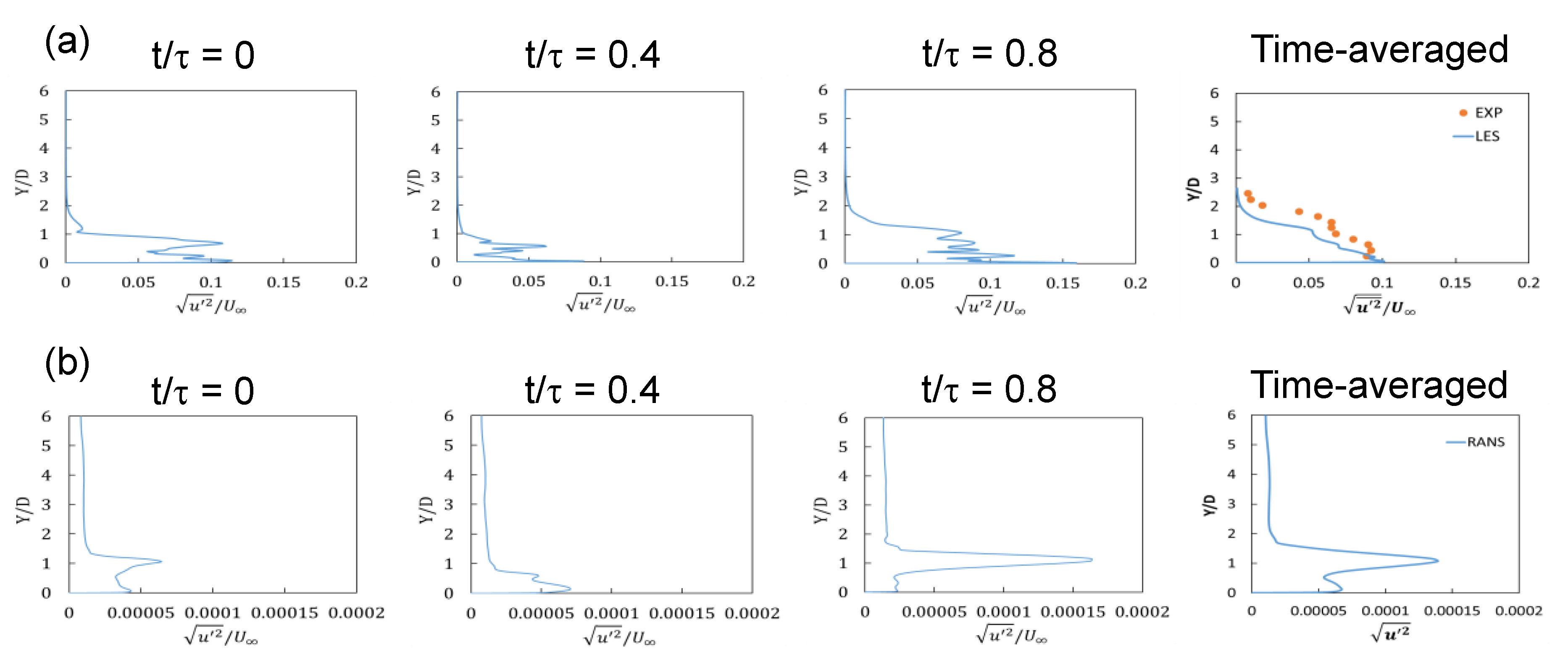
4.6. Streamwise Velocity and Fluctuation Profiles at x/D = 5 and z/D = 0

Figure 10 shows the time-averaged dimensionless streamwise velocity profiles at x/D = 5 and z/D = 0 for 0 and 32 Hz. The experimentally measured streamwise velocity profile at 0 Hz [15] has a local peak between y/D = 0 and 0.5 because of coolant jet penetration into the boundary layer. The streamwise velocity profile obtained using LES predicted this peak well, whereas the various RANS models failed to predict the peak exactly, as shown in Figure 10a. In Figure 10b, the time-averaged dimensionless streamwise velocity profiles at 32 Hz obtained by LES match well with the experimental results [15], whereas the RANS realizable k-ε model did not predict the velocity profile between y/D = 0 and 1 exactly, and the velocity gradient predicted by RANS was rather different from those in the experimental and LES results.

Figure 11 shows the time-averaged dimensionless U_rms profiles at x/D = 5 and z/D = 0 for 0 and 32 Hz. The almost-zero U_rms values obtained using the RANS realizable k-ε model are considerably much smaller than those obtained experimentally, as illustrated in the figure. The film cooling efficiency predicted using the realizable k-ε model was the closest to the experimental value, but the model yielded the weakest prediction of velocity fluctuation. As shown in Figure 11a, the time-averaged U_rms values at 0 Hz obtained by LES matched well with the experimental result. A peak of U_rms values at around y/D = 0.9 was predicted well by LES. The Reynolds stress model or the k-ω model predicted the velocity fluctuation better than the realizable k-ε, but the predicted value was still less than half the experimental value.

Figure 11b illustrates that the time-averaged U_rms values at x/D = 5 and z/D = 0 under 32 Hz pulsation obtained by LES were slightly smaller than the experimental values, even though the shape of the plot is similar to the experimental plot. Figure 11 shows that the LES approach is superior to the URANS approach in predicting the U_rms values of pulsating flows. Compared with the case of no pulsation, the turbulence intensity increased below y/D = 0.5 near the wall, and LES predicted this increase appropriately. Figure 12 illustrates the phase-averaged dimensionless U_rms profiles at x/D = 5 and z/D = 0 for 32 Hz pulsation in three phases during a period as obtained by LES and URANS.

The time-averaged dimensionless U_rms profiles at x/D = 5 and z/D = 0 as obtained by the LES Smagorinsky–Lilly model and the URANS realizable k-ε model under 32 Hz pulsation are also shown in the figure. As shown in Figure 12a, as t/τ decreases from 0 to 0.4, the y/D values corresponding to the maximum values of U_rms decrease because the heights of the large vortex at x/D = 5 decrease, as illustrated in Figure 8a. When t/τ increases from 0.4 to 0.8, the y/D values corresponding to the maximum U_rms values increase because the height of the large vortex at x/D = 5 increases. Therefore, the y/D values corresponding to the maximum U_rms values are periodic because of the outline of the large coolant vortices. This outline is attributed to the periodic blowing ratios expressed by Equation (2), even though the averaged blowing ratio is 0.5.

In terms of the point at which the turbulence intensity becomes maximum depending on the phase in Figure 12a, double peaks are observed near the wall when t/τ = 0 and around y/D = 0.7, but a single peak appears near the wall when t/τ = 0.8. The turbulence intensity of each phase obtained from RANS and shown in Figure 12b is extremely small compared to that obtained from LES. Moreover, the locations at which the maximum values of turbulence intensity occur for each phase determined using RANS are different from those determined using LES.

5. Conclusions

Numerical simulations of film cooling from a cylindrical hole on a flat plate were performed using LES under bulk flow pulsations of 32 Hz. The LES results were compared to the experimental data and the results obtained using RANS to determine whether the LES approach better predicted film cooling performance under the unsteady flow condition than the RANS method. When the pulsations were applied, the centerline and spanwise-averaged adiabatic film cooling effectiveness decreased in both the LES and RANS results, which was consistent with the experimental data. However, the RANS turbulence models overpredicted the centerline effectiveness by more than 100%, whereas the LES results deviated only marginally from the experimental data. Even in the absence of pulsation, RANS overpredicted the central temperature of the injectant and did not properly predict the mixing of the main flow and the injectant near the wall, but LES properly predicted these phenomena. In the case of pulsation of the main flow, RANS did not properly predict the injectant behavior by phase, but LES reproduced it well. The local adiabatic film cooling effectiveness predicted by LES showed a wider spread of the coolant in the spanwise direction comparing to the RANS results. The jet shear layer vortices were shown in the LES contours at z/D = 0, whereas they were not shown in the RANS contours. The Q-criterion contours obtained by LES and RANS were compared, and it was found that the LES approach predicted more diverse vortex structures as compared to the RANS method. The dimensionless streamwise velocity profiles at x/D = 5 predicted by LES at 0 and 32 Hz were considerably closer to the experimental data than the profiles predicted by RANS. Moreover, the LES approach was superior to the RANS method in predicting the dimensionless U_rms profiles. The experimental U_rms values under 32 Hz pulsation between y/d = 0 and 0.5 were higher than those between y/D = 0.5 and 1, and the U_rms profile obtained with LES was closer to the experimental data comparing to that obtained using URANS. The phase-averaged dimensionless U_rms profiles obtained using LES showed that, in each phase, the shape of the U_rms profile was attributable to the outline of the large coolant vortices.

References

1. Moran, M.; Shapiro, H.; Boettner, D.; Bailey, M. Fundamentals of Engineering Thermodynamics, 8th ed.; Wiley: New York, NY, USA, 2014. [Google Scholar]
2. Leedom, D.H.; Acharya, S. Large eddy simulations of film cooling flow fields from cylindrical and shaped holes. In ASME Turbo Expo; ASME: Berlin, Germany, 2008; pp. 865–877. [Google Scholar] [CrossRef]
3. Bogard, D.G. Airfoil film cooling. In The Gas Turbine Handbook; National Energy Technology Laboratory: Pittsburgh, PA, USA, 2006; Section 4.2.2.1. [Google Scholar]
4. Bogard, D.; Thole, K. Gas turbine film cooling. J. Propul. Power 2006, 22, 249–270. [Google Scholar] [CrossRef] [Green Version]
5. Fluent Incorporated. RAMPANT User’s Guide; Fluent Incorporated: New York, NY, USA, 1993. [Google Scholar]
6. Walters, D.K.; Leylek, J.H. Impact of film-cooling jets on turbine aerodynamic losses. ASME J. Turbomach. 2000, 122, 537–545. [Google Scholar] [CrossRef]
7. Tyagi, M.; Acharya, S. Large eddy simulation of film cooling flow from an inclined cylindrical jet. ASME J. Turbomach. 2003, 125, 734–742. [Google Scholar] [CrossRef]
8. Rozati, A.; Tafti, D. Large eddy simulation of leading edge film cooling: Part II—Heat transfer and effect of blowing ratio. In ASME Turbo Expo 2007; ASME: Montreal, QC, Canada, 2007. [Google Scholar] [CrossRef]
9. Na, S.; Shih, T. Increasing adiabatic film cooling effectiveness by using an upstream ramp. J. Heat Transfer 2007, 129, 464–471. [Google Scholar] [CrossRef]
10. Johnson, P.; Shyam, V.; Hah, C. Reynolds-Averaged Navier-Stokes Solutions to Flat Plate Film Cooling Scenarios. NASA/TM-2011-217025, 1 May 2011. [Google Scholar]
11. Wojtas, K.; Makowski, Ł.; Orciuch, W. Barium sulfate precipitation in jet reactors: Large eddy simulations, kinetics study and design considerations. Chem. Eng. Res. Des. 2020, 158, 64–76. [Google Scholar] [CrossRef]
12. Seo, H.J.; Lee, J.S.; Ligrani, P.M. The effect of injection hole length on film cooling with bulk flow pulsations. Int. J. Heat Mass Transfer 1998, 41, 3515–3528. [Google Scholar] [CrossRef]
13. Coulthard, S.; Volino, R.; Flack, K. Effect of jet pulsing on film cooling—Part I: Effectiveness and flow-field temperature results. ASME J. Turbomach. 2007, 129, 232–246. [Google Scholar] [CrossRef]
14. Nikitopoulos, D.; Acharya, S.; Oertling, J.; Muldoon, F. On active control of film-cooling flows. In ASME Turbo Expo 2006; ASME: Barcelona, Spain, 2006. [Google Scholar] [CrossRef]
15. Jung, I.S.; Ligrani, P.M.; Lee, J.S. Effects of bulk flow pulsations on phase-averaged and time-averaged film-cooled boundary layer flow structure. J. Fluids Eng. 2001, 123, 559–566. [Google Scholar] [CrossRef]
16. Han, J.; Dutta, S.; Ekkad, S. Gas Turbine Heat Transfer and Cooling Technology, 2nd ed.; CRC Press: Boca Raton, FL, USA, 2013. [Google Scholar]
17. Ansys Fluent Theory Guide, v.14. Available online: http://ansys.com/products/fluids/ansys-fluent (accessed on 7 November 2020).
18. Pointwise version 16.04. Available online: http://pointwise.com (accessed on 7 November 2020).
19. Renze, P.; Schroder, W.; Meinke, M. Large-eddy simulation of film cooling flows with variable density jets. Flow Turbul. Combust. 2008, 80, 119–132. [Google Scholar] [CrossRef]
20. Iourokina, I.; Lele, S. Towards large eddy simulation of film cooling flows on a model turbine blade leading edge. In Proceedings of the 43rd AIAA Aerospace Sciences Meeting and Exhibit, Reno, NV, USA, 10–13 January 2005. No. 2005-0670. [Google Scholar]
21. Acharya, S.; Leedom, D. Large eddy simulations of discrete hole film cooling with plenum inflow orientation effects. J. Heat Transfer 2013, 135, 011010. [Google Scholar] [CrossRef]
22. White, F. Fluid Mechanics, 8th ed.; McGraw-Hill: NewYork, NY, USA, 2015. [Google Scholar]
23. Cengel, Y.; Cimbala, J. Fluid Mechanics, 3rd ed.; McGraw-Hill: New York, NY, USA, 2014. [Google Scholar]
24. Tannehill, J.; Anderson, D.; Pletcher, R. Computational Fluid Mechanics and Heat Transfer, 2nd ed.; Taylor & Francis: Abington-on-Thames, UK, 1997. [Google Scholar]
25. Blazek, J. Computational Fluid Dynamics: Principles and Applications, 3rd ed.; Butterworth-Heinemann: Oxford, UK, 2015. [Google Scholar]
26. Jung, I.S. Effects of Bulk Flow Pulsations on Film Cooling with Compound Angle Injection Holes. Ph.D. Thesis, Seoul National University, Seoul, Korea, August 1998. [Google Scholar]
27. Hou, R.; Wen, F.; Luo, Y.; Tang, X.; Wang, S. Large eddy simulation of film cooling flow from round and trenched holes. Int. J. Heat Mass Transfer 2019, 144, 118631. [Google Scholar] [CrossRef]
28. Kolar, V. Vortex identification: New requirements and limitations. Int. J. Heat Fluid Flow 2007, 28, 638–652. [Google Scholar] [CrossRef]
29. Schroder, A.; Willert, C. (Eds.) Particle Image Velocimetry: New Developments and Recent Applications; Springer Science & Business Media: Berlin/Heidelberg, Germany, 2008; p. 382. [Google Scholar]
Figure 1. Computational domain and grid system. (a) Schematic of the computational domain (orange dashed line). (b) CFD mesh in the z/D = 0 plane. (c) CFD mesh for simulation without bulk flow pulsation. (d) Close-up of the mesh around the jet injection region.
Applsci 10 08553 g001
Figure 2. Adiabatic film cooling effectiveness at the centerline at 0 Hz (steady state) in (a) the mesh sensitivity test based on large eddy simulation (LES) calculations; (b) centerline effectiveness obtained in various Reynolds-averaged Navier–Stokes simulations (RANSs).
Applsci 10 08553 g002
Figure 3. Time-averaged centerline effectiveness at 0 and 32 Hz.
Applsci 10 08553 g003
Figure 4. Time-averaged dimensionless temperature contours at x/D = 5: (a) experiment [12]; (b) LES (Smagorinsky–Lilly); (c) RANS (realizable k-ε). Numbers in contours, 1: θ = 0.05, 2: θ = 0.1, 3: θ = 0.15, 4: θ = 0.2, 5: θ = 0.25, 6: θ = 0.3, 7: θ = 0.35, 8: θ = 0.4, 9: θ = 0.45, A: θ = 0.5, B: θ = 0.55, C: θ = 0.6, D: θ = 0.65.
Applsci 10 08553 g004
Figure 5. Phase-averaged dimensionless temperature contours at x/D = 5: (a) experiment [12]; (b) LES (Smagorinsky–Lilly); (c) RANS (realizable k-ε). Numbers in contours, 1: θ = 0.05, 2: θ = 0.1, 3: θ = 0.15, 4: θ = 0.2, 5: θ = 0.25, 6: θ = 0.3, 7: θ = 0.35, 8: θ = 0.4, 9: θ = 0.45, A: θ = 0.5, B: θ = 0.55, C: θ = 0.6, D: θ = 0.65.
Applsci 10 08553 g005
Figure 6. Time-averaged film cooling effectiveness contours on the test plate: (a) steady (0 Hz) and (b) with flow pulsation (32 Hz).
Applsci 10 08553 g006
Figure 7. Time-averaged dimensionless temperature contours at z/D = 0: (a) steady (0 Hz) and (b) with flow pulsation (32 Hz).
Applsci 10 08553 g007
Figure 8. Phase-averaged dimensionless temperature contours at y/D = 0 (upper) and z/D = 0 (lower) for 32 Hz: (a) LES (Smagorinsky–Lilly) and (b) unsteady RANS (URANS) (realizable k-ε).
Applsci 10 08553 g008
Figure 9. Q-criterion contours colored by y-vorticity in each phase with iso-surfaces of level 1000 for three dimensions under 32 Hz pulsation: (a) LES (Smagorinsky–Lilly) and (b) unsteady RANS (realizable k-ε).
Applsci 10 08553 g009
Figure 10. Time-averaged streamwise velocity profiles at x/D = 5 and z/D = 0: (a) 0 Hz and (b) 32 Hz.
Applsci 10 08553 g010
Figure 11. Time-averaged dimensionless Urms profiles obtained using RANS and LES models at x/D = 5 and z/D = 0: (a) 0 Hz and (b) 32 Hz.
Applsci 10 08553 g011
Figure 12. Phase-averaged dimensionless Urms profiles at x/D = 5 and z/D = 0 for 32 Hz: (a) LES (Smagorinsky–Lilly) and (b) URANS (realizable k-ε).
Applsci 10 08553 g012