A Deep Learning Approach with Feature Derivation and Selection for Overdue Repayment Forecasting

 ,
,  ,
,
Abstract
1. Introduction
- We present a new dataset that originates from a practical application scenario in online lending, which can be downloaded at https://github.com/zjersey/payment_overdue_dataset. Over one million repayment records of 85,000 anonymous borrowers are contained, and all the sensitive information is encrypted for confidentiality.
- An improved feature derivation and selection method is proposed that can generate extensive, fully-combined new features and select an arbitrary number of the most significant features based on a scorecard model.
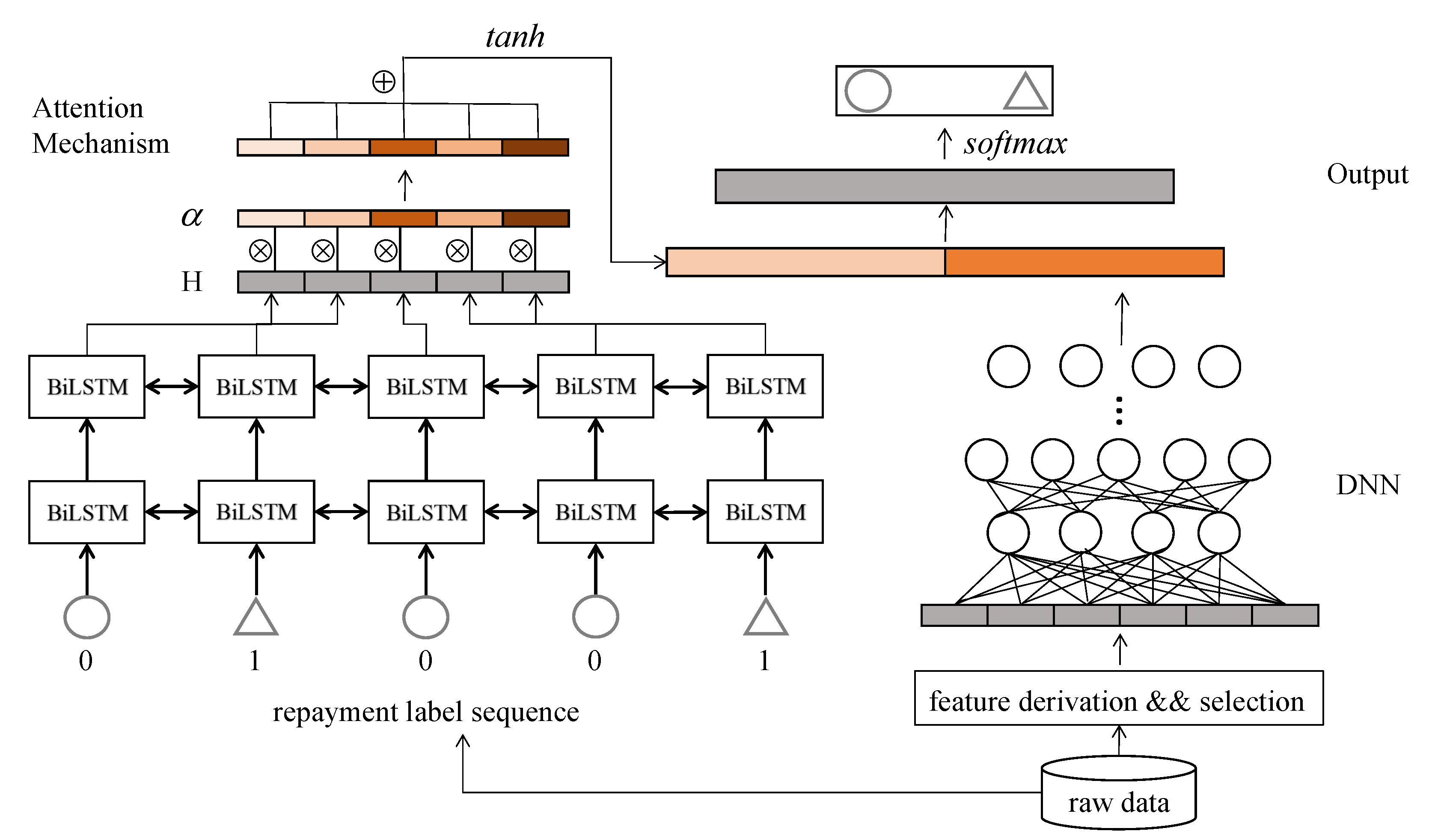
- We introduce deep learning models into the domain of risk control in online lending; specifically, overdue repayment forecasting based on historical repayment behaviors. Our proposed architecture, namely AD-BLSTM, combines a deep neural network (DNN), bidirectional long short-term memory (LSTM) [6] (BiLSTM) and the attention mechanism [7]. DNN and BiLSTM are used to learn from the static background information and dynamic event sequence, respectively, to maximize the superiority of the two networks. The attention mechanism is introduced to weight the importance of hidden layers in LSTM and integrate them to obtain a more informative representation.
- Experimental results demonstrate that our approach outperforms various general machine learning models and neural network models. Interpretability improvement work is implemented based on the attention mechanism and derived features. We visualize differentiated attention weights to explore the key event time steps and analyze the feature importance of derived features to determine the causes of overdue repayment.
2. Related Work
2.1. Event Prediction
2.2. Deep Learning in Online Lending
3. Proposed System
3.1. Feature Derivation and Selection
| Algorithm 1: Feature Selection. |
 |
3.2. DNN Layer
3.3. Multi-BiLSTM Layer
3.4. Attention Layer
3.5. Output Layer
4. Experiments
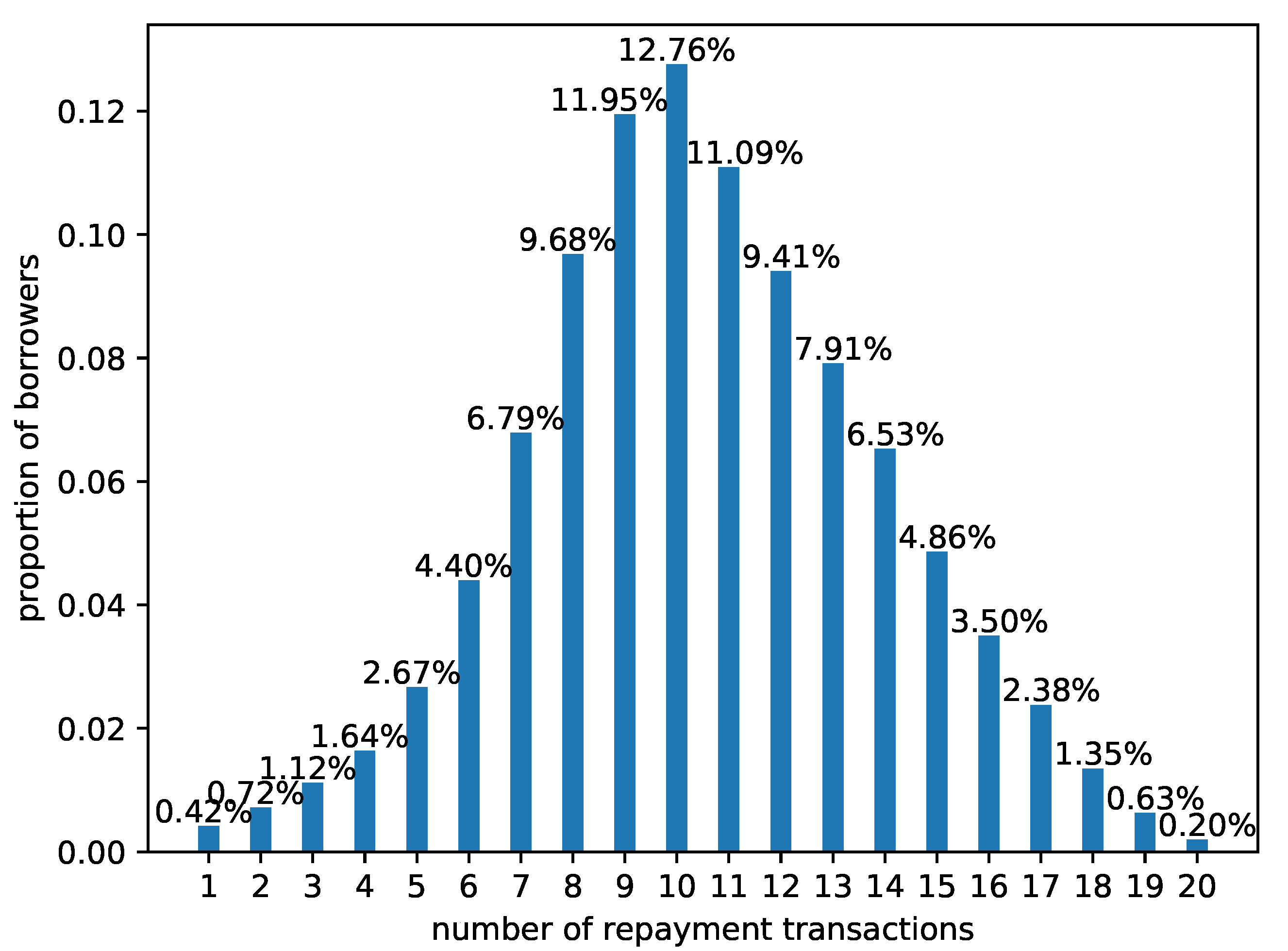
4.1. Dataset
- Customer information (after data masking): borrowers’ unique identification, industry, etc. Note that data masking has been applied to protect the privacy of customers.
- Dynamic repayment records: obliged repayment amount, obliged repayment time, overdue days, etc.
- Background information: expense ratio, loan type, order scenario, etc.
4.2. Data Preprocessing and Experimental Settings
4.3. Evaluation Indicators
- TP: True positive, showing that the actual value and prediction value are both positive.
- TN: True negative, showing that the actual value and prediction value are both negative.
- FP: False positive, showing that the actual value is negative while the prediction value is positive.
- FN: False negative, showing that the actual value is positive while the prediction value is negative.
4.4. Baselines
- Logistic regression (LR) is a fundamental and commonly used classification approach based on sigmoid function and the maximum likelihood method. The LR model does not need to assume the prior distribution of input data. Not only can the classification label be determined, but the predicted probability can also be obtained. and so the threshold can be adjusted according to demand and label distribution.
- XGBoost [46] achieved state-of-the-art performance in large numbers of machine learning tasks as soon as it was proposed. The overall idea of XGBoost is to constantly add new decision trees to improve the performance of a system. Newly supplied trees can make up for the shortcomings of the previous weak classifiers to compensate for prediction residuals.
- The factorization machine (FM) [47] interactively combines input features in pairs, which allows training to be performed on each pair of potential features. There is a similarity between FM and SVM in the formula. However, in contrast to SVM, all interactions between features are considered via factorized parameters in FM, and so FM works well even in problems with huge sparsity.
- DNN extracts derived and selected features directly and connects them to the output layer.
- In multi-BiRNN, we consider each variable of the input record as a dynamic variable and feed input data into a two-layer bidirectional RNN. We choose this structure due to its similarity to the LSTM layer in AD-BLSTM, thus facilitating comparison.
- Multi-BiLSTM has the same structure as multi-BiRNN except that the RNN is replaced with LSTM.
4.5. Result Analysis
4.6. Ablation Study
4.7. Interpretability
4.7.1. Locating Critical Time Point via the Attention Mechanism
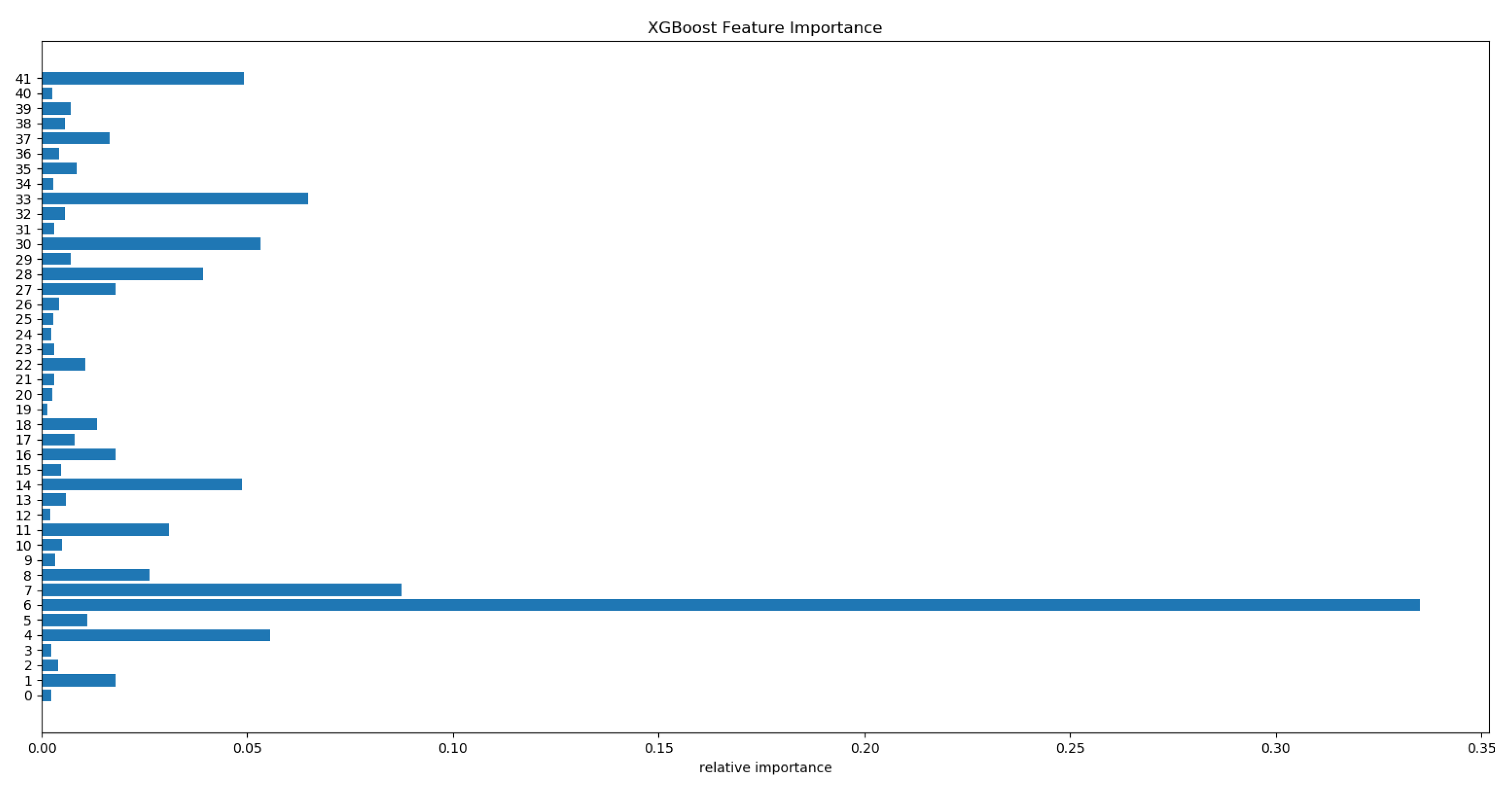
4.7.2. Analysis of Derived Features
5. Conclusions
Author Contributions
Funding
Conflicts of Interest
References
- Yan, J.; Zhang, C.; Zha, H.; Gong, M.; Sun, C.; Huang, J.; Chu, S.; Yang, X. On machine learning towards predictive sales pipeline analytics. In Proceedings of the Twenty-Ninth AAAI Conference on Artificial Intelligence, Austin, TX, USA, 25–30 January 2015. [Google Scholar]
- Metzger, A.; Leitner, P.; Ivanović, D.; Schmieders, E.; Franklin, R.; Carro, M.; Dustdar, S.; Pohl, K. Comparing and combining predictive business process monitoring techniques. IEEE Trans. Syst. Man Cybern. Syst. 2014, 45, 276–290. [Google Scholar] [CrossRef]
- Wang, W.; Zhang, W.; Wang, J.; Yan, J.; Zha, H. Learning sequential correlation for user generated textual content popularity prediction. In Proceedings of the 2018 International Joint Conference on Artificial Intelligence (IJCAI), Stockholm, Sweden, 13–19 July 2018; pp. 1625–1631. [Google Scholar]
- Xiao, S.; Yan, J.; Li, C.; Jin, B.; Wang, X.; Yang, X.; Chu, S.M.; Zha, H. On modeling and predicting individual paper citation count over time. In Proceedings of the 2016 International Joint Conference on Artificial Intelligence (IJCAI), New York, NY, USA, 9–15 July 2016; pp. 2676–2682. [Google Scholar]
- Liu, X.; Yan, J.; Xiao, S.; Wang, X.; Zha, H.; Chu, S.M. On predictive patent valuation: Forecasting patent citations and their types. In Proceedings of the Thirty-First AAAI Conference on Artificial Intelligence, San Francisco, CA, USA, 4–10 February 2017. [Google Scholar]
- Hochreiter, S.; Schmidhuber, J. Long short-term memory. Neural Comput. 1997, 9, 1735–1780. [Google Scholar] [CrossRef] [PubMed]
- Bahdanau, D.; Cho, K.; Bengio, Y. Neural machine translation by jointly learning to align and translate. In Proceedings of the 3rd International Conference on Learning Representations (ICLR) 2015, San Diego, CA, USA, 7–9 May 2015. [Google Scholar]
- Becker, J.; Breuker, D.; Delfmann, P.; Matzner, M. Designing and implementing a framework for event-based predictive modelling of business processes. In Enterprise Modelling and Information Systems Architectures-EMISA 2014; Gesellschaft für Informatik eV: Bonn, Germany, 2014. [Google Scholar]
- Moon, T.K. The expectation-maximization algorithm. IEEE Signal Process. Mag. 1996, 13, 47–60. [Google Scholar] [CrossRef]
- Breuker, D.; Matzner, M.; Delfmann, P.; Becker, J. Comprehensible Predictive Models for Business Processes. MIS Q. 2016, 40, 1009–1034. [Google Scholar] [CrossRef]
- Chater, N.; Manning, C.D. Probabilistic models of language processing and acquisition. Trends Cogn. Sci. 2006, 10, 335–344. [Google Scholar] [CrossRef] [PubMed]
- De Weerdt, J.; De Backer, M.; Vanthienen, J.; Baesens, B. A multi-dimensional quality assessment of state-of-the-art process discovery algorithms using real-life event logs. Inf. Syst. 2012, 37, 654–676. [Google Scholar] [CrossRef]
- Folino, F.; Guarascio, M.; Pontieri, L. Discovering context-aware models for predicting business process performances. In Proceedings of the OTM Confederated International Conferences “On the Move to Meaningful Internet Systems”, Rome, Italy, 10–14 September 2012; Springer: Berlin/Heidelberg, Germany, 2012; pp. 287–304. [Google Scholar]
- Li, L.; Yan, J.; Yang, X.; Jin, Y. Learning interpretable deep state space model for probabilistic time series forecasting. In Proceedings of the 2019 International Joint Conference on Artificial Intelligence (IJCAI), Macao, China, 10–16 August 2019; pp. 2901–2908. [Google Scholar]
- Quinlan, J.R. C4. 5: Programs for Machine Learning; Elsevier: Amsterdam, The Netherlands, 2014. [Google Scholar]
- Cortes, C.; Vapnik, V. Support-vector networks. Mach. Learn. 1995, 20, 273–297. [Google Scholar] [CrossRef]
- Friedman, N.; Geiger, D.; Goldszmidt, M. Bayesian network classifiers. Mach. Learn. 1997, 29, 131–163. [Google Scholar] [CrossRef]
- Kaufman, L.; Rousseeuw, P.J. Finding Groups in Data: An Introduction to Cluster Analysis; John Wiley & Sons: Hoboken, NJ, USA, 2009; Volume 344. [Google Scholar]
- Elman, J.L. Finding structure in time. Cogn. Sci. 1990, 14, 179–211. [Google Scholar] [CrossRef]
- Mikolov, T.; Karafiát, M.; Burget, L.; Černockỳ, J.; Khudanpur, S. Recurrent neural network based language model. In Proceedings of the Eleventh Annual Conference of the International Speech Communication Association, Chiba, Japan, 26–30 September 2010. [Google Scholar]
- Sundermeyer, M.; Schlüter, R.; Ney, H. LSTM neural networks for language modeling. In Proceedings of the Thirteenth Annual Conference of the International Speech Communication Association, Portland, OR, USA, 9–13 September 2012. [Google Scholar]
- Cho, K.; Van Merriënboer, B.; Gulcehre, C.; Bahdanau, D.; Bougares, F.; Schwenk, H.; Bengio, Y. Learning phrase representations using RNN encoder-decoder for statistical machine translation. arXiv 2014, arXiv:1406.1078. [Google Scholar]
- Li, L.; Yan, J.; Wang, H.; Jin, Y. Anomaly Detection of Time Series With Smoothness-Inducing Sequential Variational Auto-Encoder. IEEE Trans. Neural Netw. Learn. Syst. 2020. [Google Scholar] [CrossRef] [PubMed]
- Wang, G.; Qin, Z.; Yan, J.; Jiang, L. Learning to select elements for graphic design. In Proceedings of the 2020 International Conference on Multimedia Retrieval, Dublin, Ireland, 8–11 June 2020; pp. 91–99. [Google Scholar]
- Evermann, J.; Rehse, J.R.; Fettke, P. A deep learning approach for predicting process behaviour at runtime. In Proceedings of the 2016 International Conference on Business Process Management, Rio de Janeiro, Brazil, 18–22 September 2016; Springer: Berlin/Heidelberg, Germany, 2016; pp. 327–338. [Google Scholar]
- Tax, N.; Verenich, I.; La Rosa, M.; Dumas, M. Predictive business process monitoring with LSTM neural networks. In Proceedings of the 2017 International Conference on Advanced Information Systems Engineering, Essen, Germany, 12–16 June 2017; Springer: Berlin/Heidelberg, Germany, 2017; pp. 477–492. [Google Scholar]
- Polato, M.; Sperduti, A.; Burattin, A.; de Leoni, M. Time and activity sequence prediction of business process instances. Computing 2018, 100, 1005–1031. [Google Scholar] [CrossRef]
- Rogge-Solti, A.; Weske, M. Prediction of remaining service execution time using stochastic petri nets with arbitrary firing delays. In Proceedings of the 2013 International Conference on Service-Oriented Computing, Berlin, Germany, 2–5 December 2013; Springer: Berlin/Heidelberg, Germany, 2013; pp. 389–403. [Google Scholar]
- Maggi, F.M.; Di Francescomarino, C.; Dumas, M.; Ghidini, C. Predictive monitoring of business processes. In Proceedings of the 2014 International Conference on Advanced Information Systems Engineering, Thessaloniki, Greece, 16–20 June 2014; Springer: Berlin/Heidelberg, Germany, 2014; pp. 457–472. [Google Scholar]
- Yan, J.; Liu, X.; Shi, L.; Li, C.; Zha, H. Improving maximum likelihood estimation of temporal point process via discriminative and adversarial learning. In Proceedings of the 2018 International Joint Conference on Artificial Intelligence (IJCAI), Stockholm, Sweden, 13–19 July 2018; pp. 2948–2954. [Google Scholar]
- Wu, W.; Yan, J.; Yang, X.; Zha, H. Reinforcement Learning with Policy Mixture Model for Temporal Point Processes Clustering. arXiv 2019, arXiv:1905.12345. [Google Scholar]
- Xiao, S.; Farajtabar, M.; Ye, X.; Yan, J.; Song, L.; Zha, H. Wasserstein learning of deep generative point process models. In Proceedings of the Advances in Neural Information Processing Systems 2017, Long Beach, CA, USA, 4–9 December 2017; pp. 3247–3257. [Google Scholar]
- Wu, W.; Yan, J.; Yang, X.; Zha, H. Decoupled learning for factorial marked temporal point processes. In Proceedings of the 24th ACM SIGKDD International Conference on Knowledge Discovery & Data Mining, London, UK, 19–23 August 2018; pp. 2516–2525. [Google Scholar]
- Xiao, S.; Yan, J.; Farajtabar, M.; Song, L.; Yang, X.; Zha, H. Learning time series associated event sequences with recurrent point process networks. IEEE Trans. Neural Netw. Learn. Syst. 2019, 30, 3124–3136. [Google Scholar] [CrossRef] [PubMed]
- Yan, J.; Xu, H.; Li, L. Modeling and applications for temporal point processes. In Proceedings of the 25th ACM SIGKDD International Conference on Knowledge Discovery & Data Mining, Anchorage, AK, USA, 4–8 August 2019; ACM: New York, NY, USA, 2019; pp. 3227–3228. [Google Scholar]
- Xiao, S.; Xu, H.; Yan, J.; Farajtabar, M.; Yang, X.; Song, L.; Zha, H. Learning conditional generative models for temporal point processes. In Proceedings of the Thirty-Second AAAI Conference on Artificial Intelligence, New Orleans, LA, USA, 2–7 February 2018. [Google Scholar]
- Xiao, S.; Yan, J.; Yang, X.; Zha, H.; Chu, S.M. Modeling the intensity function of point process via recurrent neural networks. In Proceedings of the Thirty-First AAAI Conference on Artificial Intelligence, San Francisco, CA, USA, 4–9 February 2017. [Google Scholar]
- Wu, Q.; Zhang, Z.; Gao, X.; Yan, J.; Chen, G. Learning latent process from high-dimensional event sequences via efficient sampling. In Proceedings of the 2019 Advances in Neural Information Processing Systems, Vancouver, BC, Canada, 8–14 December 2019; pp. 3847–3856. [Google Scholar]
- Wu, W.; Yan, J.; Yang, X.; Zha, H. Discovering Temporal Patterns for Event Sequence Clustering via Policy Mixture Model. IEEE Trans. Knowl. Data Eng. 2020. [Google Scholar] [CrossRef]
- Wang, C.; Han, D.; Liu, Q.; Luo, S. A deep learning approach for credit scoring of Peer-to-Peer lending using attention mechanism LSTM. IEEE Access 2018, 7, 2161–2168. [Google Scholar] [CrossRef]
- Mikolov, T.; Sutskever, I.; Chen, K.; Corrado, G.S.; Dean, J. Distributed representations of words and phrases and their compositionality. In Proceedings of the 2013 Advances in Neural Information Processing Systems, Lake Tahoe, NV, USA, 5–8 December 2013; pp. 3111–3119. [Google Scholar]
- Fu, X.; Zhang, S.; Chen, J.; Ouyang, T.; Wu, J. A Sentiment-Aware Trading Volume Prediction Model for P2P Market Using LSTM. IEEE Access 2019, 7, 81934–81944. [Google Scholar] [CrossRef]
- Kim, Y. Convolutional neural networks for sentence classification. In Proceedings of the 2014 Conference on Empirical Methods in Natural Language Processing (EMNLP), Doha, Qatar, 25–29 October 2014; pp. 1746–1751. [Google Scholar]
- Kerber, R. Chimerge: Discretization of numeric attributes. In Proceedings of the Tenth National Conference on Artificial Intelligence, San Jose, CA, USA, 12–16 July 1992; pp. 123–128. [Google Scholar]
- Peters, M.E.; Neumann, M.; Iyyer, M.; Gardner, M.; Clark, C.; Lee, K.; Zettlemoyer, L. Deep contextualized word representations. In Proceedings of the Annual Conference of the North American Chapter of the Association for Computational Linguistics: Human Language Technologies (NAACL-HLT), New Orleans, LA, USA, 1–6 June 2018; pp. 2227–2237. [Google Scholar]
- Chen, T.; Guestrin, C. Xgboost: A scalable tree boosting system. In Proceedings of the 22nd ACM Sigkdd International Conference on Knowledge Discovery and Data Mining, San Francisco, CA, USA, 13–17 August 2016; ACM: New York, NY, USA, 2016; pp. 785–794. [Google Scholar]
- Rendle, S. Factorization machines. In Proceedings of the IEEE International Conference on Data Mining, Vancouver, BC, Canada, 11–14 December 2011. [Google Scholar]


| Parameter | Parameter Description | Value |
|---|---|---|
| time_step | Length of input sequence | 15 |
| lr | Learning rate | 0.03 |
| optimizer | Optimization method | Adam |
| lstm_unit | Neuron number in single LSTM | 50 |
| DNN_units | Neuron numbers in hidden layers of DNN | [150, 300] |
| epoch | Training rounds | 20 |
| batch_size | Batch size | 128 |
| dropout | Dropout ratio of LSTM | 0.15 |
| Methods | Accuracy | Recall | AUC | KS |
|---|---|---|---|---|
| LR | 0.850 | 0.18 | 0.675 | 0.286 |
| XGBoost | 0.851 | 0.19 | 0.684 | 0.292 |
| FM | 0.852 | 0.21 | 0.684 | 0.304 |
| DNN | 0.852 | 0.23 | 0.685 | 0.315 |
| Multi-BiRNN | 0.798 | 0.43 | 0.779 | 0.432 |
| Multi -BiLSTM | 0.804 | 0.47 | 0.781 | 0.438 |
| AD-BLSTM | 0.855 | 0.59 | 0.844 | 0.481 |
| Model | Accuracy | Recall | AUC | KS |
|---|---|---|---|---|
| AD-BLSTM | 0.855 | 0.59 | 0.844 | 0.481 |
| ↪w/o attention | 0.857 | 0.57 | 0.843 | 0.478 |
| ↪w/o derivation | 0.840 | 0.57 | 0.842 | 0.477 |
| ↪w/o attention and derivation | 0.842 | 0.53 | 0.840 | 0.473 |
| ↪w/o sequence | 0.852 | 0.23 | 0.685 | 0.315 |
| ↪w/o statics | 0.785 | 0.41 | 0.747 | 0.416 |
Publisher’s Note: MDPI stays neutral with regard to jurisdictional claims in published maps and institutional affiliations. |
© 2020 by the authors. Licensee MDPI, Basel, Switzerland. This article is an open access article distributed under the terms and conditions of the Creative Commons Attribution (CC BY) license (http://creativecommons.org/licenses/by/4.0/).
Share and Cite
Liu, B.; Zhang, Z.; Yan, J.; Zhang, N.; Zha, H.; Li, G.; Li, Y.; Yu, Q. A Deep Learning Approach with Feature Derivation and Selection for Overdue Repayment Forecasting. Appl. Sci. 2020, 10, 8491. https://doi.org/10.3390/app10238491
Liu B, Zhang Z, Yan J, Zhang N, Zha H, Li G, Li Y, Yu Q. A Deep Learning Approach with Feature Derivation and Selection for Overdue Repayment Forecasting. Applied Sciences. 2020; 10(23):8491. https://doi.org/10.3390/app10238491
Chicago/Turabian StyleLiu, Bin, Zhexi Zhang, Junchi Yan, Ning Zhang, Hongyuan Zha, Guofu Li, Yanting Li, and Quan Yu. 2020. "A Deep Learning Approach with Feature Derivation and Selection for Overdue Repayment Forecasting" Applied Sciences 10, no. 23: 8491. https://doi.org/10.3390/app10238491
APA StyleLiu, B., Zhang, Z., Yan, J., Zhang, N., Zha, H., Li, G., Li, Y., & Yu, Q. (2020). A Deep Learning Approach with Feature Derivation and Selection for Overdue Repayment Forecasting. Applied Sciences, 10(23), 8491. https://doi.org/10.3390/app10238491