Article

Automatic Fabric Defect Detection Method Using PRAN-Net

1
Institute of Microelectronics of the Chinese Academy of Sciences, Beijing 100029, China
2
University of Chinese Academy of Sciences, Beijing 100049, China
3
School of Instrumentation and Optoelectronic Engineering, Beihang University, Beijing 100083, China
*
Author to whom correspondence should be addressed.
Appl. Sci. 2020, 10(23), 8434; https://doi.org/10.3390/app10238434
Submission received: 5 November 2020 / Revised: 24 November 2020 / Accepted: 25 November 2020 / Published: 26 November 2020

Abstract

:
Fabric defect detection is very important in the textile quality process. Current deep learning algorithms are not effective in detecting tiny and extreme aspect ratio fabric defects. In this paper, we proposed a strong detection method, Priori Anchor Convolutional Neural Network (PRAN-Net), for fabric defect detection to improve the detection and location accuracy of fabric defects and decrease the inspection time. First, we used Feature Pyramid Network (FPN) by selected multi-scale feature maps to reserve more detailed information of tiny defects. Secondly, we proposed a trick to generate sparse priori anchors based on fabric defects ground truth boxes instead of fixed anchors to locate extreme defects more accurately and efficiently. Finally, a classification network is used to classify and refine the position of the fabric defects. The method was validated on two self-made fabric datasets. Experimental results indicate that our method significantly improved the accuracy and efficiency of detecting fabric defects and is more suitable to the automatic fabric defect detection.

1. Introduction

Fabric defect detection is a necessary quality inspection process, which aims to classify and locate defects in textiles. However, most fabric defects are categorized by the human vision, the inspection accuracy of which is only 50–70% [1] and the inspection speed of which is only 6–8 m per minute [2]. Automatic defect detection technology based on deep learning dramatically improves the defects detection accuracy and efficiency. Therefore, the research of the automatic fabric defect inspection algorithms has been paid more and more attention.
However, there are more than 70 categories of fabric defects [3] in actual production. Most of them are tiny and have extreme aspect ratios in images, such as coarse warp, coarse weft and mispick. Currently, deep learning algorithms aiming to object detection are divided into one-stage algorithms [4,5,6,7,8,9] and two-stage algorithms. One-stage algorithms such as RetinaNet have fast inspection speed which meets the demands of on-line inspection, however its detection accuracy is not satisfied. Compared with one-stage algorithms, two-stage algorithms [10,11,12,13,14,15] have higher accuracy and positioning in objects detection. Faster R-CNN [13], as an excellent two-stage algorithm, is easy to implement and has high accuracy on multiple objects detection, many researchers use the network model for ship detection [16] and medical image detection [17,18]. However, the detected objects occupy larger regions in images, and the shapes of the detected objects are moderate aspect ratios, such as people, airplanes, etc. Many methods, such as GAN [19], deep convolutional neural network [20] and YOLO v3 [21], are effective in detecting fabric defects, but cannot detect exceedingly small and extreme aspect ratios fabric defects well.
To improve the detection accuracy of tiny defects, some researchers use Feature Pyramid Network (FPN) [22] to fuse feature maps of different scales. The Mask RCNN [14] method improves the tiny defects detection accuracy, but the runtime of detection is much longer. Although these methods improve the detection accuracy of tiny defects, its location accuracy for extreme shape defects is still unsatisfied, because the preset fixed size anchors cannot accurately match extreme aspect ratios fabric defects in images.
Anchor-free algorithms such as CenterNet [23] assume object as a point to improve the detection accuracy of tiny objects and partly improve the detection ability of extreme objects. However, for extreme long and narrow fabric defects, CenterNet still cannot detect them accurately. A Guided Anchoring method [24] is proposed instead of fixed anchors, which decreases the detection speed and increases the detection accuracy of the extreme defects. However, the Guided Anchoring method cannot detect defects when defects distribution is too concentrated.
Inspired by the FPN and the Guided Anchoring, this paper proposes a Priori Anchor Convolutional Neural Network (PRAN-Net) based on Faster R-CNN to detect tiny and extreme fabric defects. Firstly, we introduce the FPN to reserve more detailed information, which adapts to tiny fabric defects. Secondly, we proposed a trick to generate sparse priori anchors, which can match extreme aspect ratio defects well and remove a large number of redundant anchors in order to improve the accuracy and efficiency of the fabric defect detection. Finally, a classification network is used to classify and refine the position of the fabric defects.

2. PRAN-Net Fabric Defect Detection Method Based on Faster R-CNN

Figure 1 shows the fabric defect detection process of the PRAN-Net based on the Faster R-CNN proposed in this paper. First, the FPN [22] is used to extract feature maps at different scales from the fabric images. Then, priori anchors are adaptively generated in each scale feature map as the defect proposals. Finally, a classification network is established to classify and refine the position of defects in fabric images by the defect proposals.

2.1. Feature Extraction Based on Multi-Scales Feature Maps

As shown in Figure 2, we use the typical deep residual network ResNet-101-FPN [25] as the backbone to extract features of fabric defects. The whole network is divided into bottom-upline and top-down line, which consists of several convolutional layers and upsampling layers. These two lines are laterally connected with 1 × 1 convolutional layers, which are used to reduce the channel dimensions. For the bottom-upline, the classical FPN obtain five scales feature maps. To reserve enough information of tiny defects while getting rid of redundant information and increasing efficiency, we only retain three feature maps with strides of {4, 8, 32} defined as {C1, C2, C3}, respectively. For the top-down line, the high-level feature map is fused with the low-level feature map. M3 is the third scale feature map in the merged maps obtained by the 1 × 1 convolution of C3. The upsampled M3 and the 1 × 1 convolution result of C3 are summed to get M2. The same operation is done to M2 and C2 to get M1. To reduce the aliasing effect of upsampling, {M1, M2, M3} are convoluted by a 3 × 3 convolution kernel to get three new feature maps {P1, P2, P3}. The top-down line operation enables to reserve more detailed information of defects by interlayer fusion, which is especially beneficial to detect tiny defects.

2.2. Priori Anchor Generation

Region Proposal Network (RPN) [13] is used to predict defect proposals in feature maps by anchors. Generally, a series of fixed-size anchors set for each pixel of the feature map in RPN work well to detect the moderate aspect ratio defects. Due to the extreme aspect ratios of most fabric defects, fixed-size anchors cannot match defective regions exactly, which lead to defect location deviation. Furthermore, a large number of fixed anchors are set in each feature map by sliding windows, most of which have no contribution to detect defects and lead to extra calculation time. PRAN-Net generates sparse priori anchors in images to locate diverse fabric defects accurately and efficiently.
The fabric defect in images determined by the location and the shape is represented by a quaternary tuple x , y , w , h , where x , y is the center coordinate of the defect, w and h are the width and height of the defect, respectively. Assuming that the probability of a defect x , y , w , h locating in the image I satisfies the following condition:
p ( x , y , w , h | I ) = p ( x , y | I ) p ( w , h | x , y , I )
where p ( x , y | I ) is the probability of the existing defect in the image I , and p ( w , h | x , y , I ) is the probability of the specific shape w , h defects. Based on formula (1), the priori anchors are generated adaptively in different scale feature maps in two steps: predicting coordinates of the defect center and predicting the shape of the defect guided by the ground truth (GT) box of defect as shown in Figure 3.

2.2.1. Location Prediction

The first step is to predict the location of the priori anchor in each feature map by the location prediction network N l as shown in Figure 3. The semantic segmentation is made to get the defective score map by a 1 × 1 convolutional layer. Then, the defective scores are transformed by an element-wised sigmoid function to get the defective probability map with the same size as the feature map. The pixels whose value are larger than the set threshold Δ L are considered as the defect pixels. We determine the defect sub-regions by gathering the defect pixels within the set distance between the adjacent pixels. The GT box, presented by g t = ( x g , y g , w g , h g ) is the labeled defect in the original fabric image, where x g and y g are the center coordinates of the GT, w g and h g are the width and height of the GT, respectively. The GT box is mapped to each feature map as GT’, presented by g t = ( x g , y g , w g , h g ) , where ( x g , y g ) and ( w g , h g ) are the center coordinates and the shape. If ( x g , y g ) is in one of the sub-regions, the enclosing rectangle of this sub-region is taken as the candidate anchor, which is described as a c a n = { ( x 0 , y 0 , w 0 , h 0 ) | w 0 > 0 , h 0 > 0 } , where ( x 0 , y 0 ) are the center coordinates, w 0 and h 0 are the width and height of the candidate anchor. We introduce GHM-C loss L l o c [26] as the priori anchor location loss.

2.2.2. Shape Prediction

As shown in Figure 3, the second step is to predict the shape of the priori anchors a p r i o r i . The I o U c a n is the intersection over union (IoU) of the candidate anchor and the matched GT’. We try to make the IoU larger by adjusting the width and height of the candidate anchor. First the shape prediction network N s , which includes a 1 × 1 convolutional layer and an element-wise transform layer is used to predict the width w 0 and height h 0 as follows:
w 0 = w 0 e t w
h 0 = h 0 e t h
where t w and t h are the scale parameters obtained by the above 1 × 1 convolution layer. Adjust w 0 and h 0 until the adjusted candidate anchor demands the following condition:
I o U ( a p r i o r i , g t ) = max ( I o U c a n ( a c a n , g t ) )
The last width w 0 and height h 0 is the shape of the priori anchor. Different from thousands of fixed anchors for each feature map, only sparse prior anchors are generated by PRAN-Net. The priori anchor shape loss L s h a p e is as follows:
L s h a p e = s m o o t h L 1 ( 1 min ( w g w 0 , w 0 w g ) ) + s m o o t h L 1 ( 1 min ( h g h 0 , h 0 h g ) )

2.3. Defect Classification Network

The structure of the classification network is shown in Figure 4. Defect proposals and their corresponding feature maps are resized by a RoI Align layer [14] to the fixed size. Then, the features are fed into a sequence of full-connection layers and are finally branched to classification and bounding box regression. The classification branch outputs the prediction of defect category, and the regression branch outputs the prediction of defect position after the secondary location.
We introduce the softmax loss as the classification loss L c l s and the smooth L1 loss as the bounding box regression loss L r e g to supervise the classification network loss of fabric defects.
The total loss L is the sum of the priori anchor location loss L l o c , the priori anchor shape loss L s h a p e , the classification loss L c l s and the bounding box regression loss L r e g , as follows:
L = L l o c + L s h a p e + L c l s + L r e g

3. Experiment and Results

The fabric defects detection experiments environment is Intel Core I7 v4 CPU, graphics card RTX2080Ti GPU, 128GB RAM and Ubuntu 16.04 operating system. All experiments are implemented by the Pytorch. There are two experimental fabric defect datasets: the plain fabric dataset and the denim dataset.

3.1. Experimental Datasets

3.1.1. The Plain Fabric Dataset

The plain fabric dataset has 1054 images and overall 1164 defects labeled in PASCAL VOC [27] format. The image size is 128 × 256 pixels. There are five categories of defects which are oil stains, coarse warp, long coarse weft, short coarse weft and mispick, respectively, as shown in Figure 5. It can be seen that most defects are tiny and the shape of the defects are diverse. Table 1 gives the number of each defect category. All defects except oil stains are tiny. Long coarse weft, coarse warp and mispick are the extreme aspect ratio defects, which made up 54.4% of the total defects.

3.1.2. The Denim Dataset

The denim dataset has 6913 images and overall 9523 defects labeled in PASCAL VOC [27] format. The image size is 2446 × 1000 pixels. There are 20 categories of defects. The number of each category defect is shown in Table 2 and Figure 6a. Most of the defects are tiny, and there areas are less than 1% of the entire image. The aspect ratios distribution of defects is shown in Figure 6b. The red bounding box corresponds to the number of defects with moderate aspect ratios. The extreme aspect ratio defects from 0 to 0.5 and 2 to 5 are accounted for 47.7% of total defects.
Figure 7 shows some defects of the denim dataset. Defects such as knot and coarse warp in images are extremely small, the shapes of three wire and flower jump defects are extreme aspect ratios outside the red box in Figure 6b.

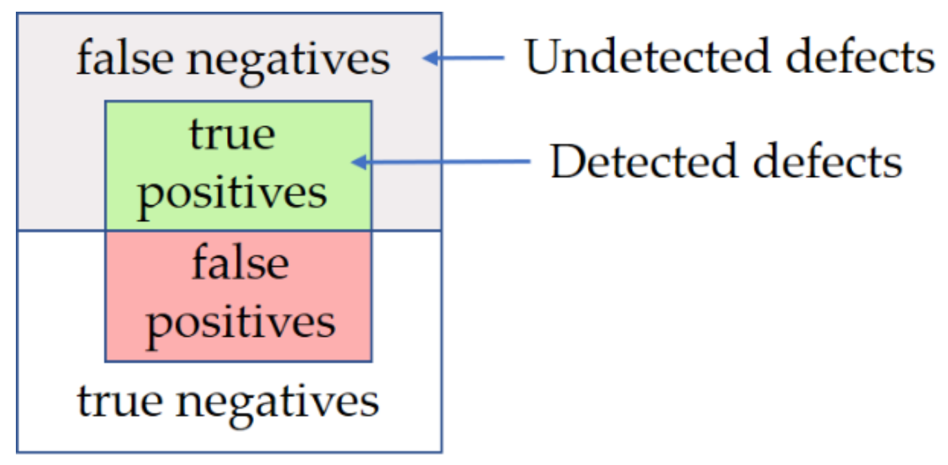
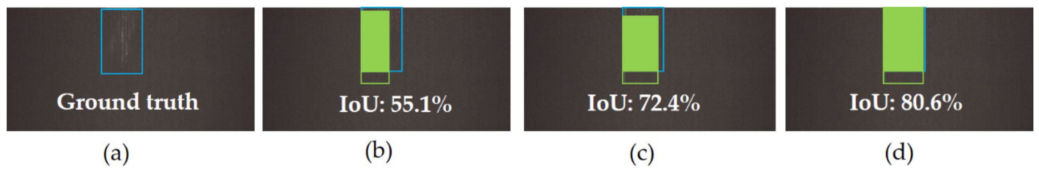
3.2. Defect Detection Evaluation Metrics

IoU of the detected region with the matched GT is used to evaluate detection performance as shown in Figure 8. The IoU threshold is set to 0.5 to distinguish whether the detected bounding box is a defect.
The detection results of each category defect are divided into true positive (TP), false positive (FP), true negative (TN) and false negative (FN) as shown in Figure 9. The upper of the outer rectangle is true defects including TP and FN, the lower of the outer rectangle is non-defects including FP and TN. The inner rectangle is the detected defects, which includes TP and FP detected by mistake.
We use Accuracy (ACC), mean Average Precision (mAP), Average Recall (AR), Average IoU of the detected defects, ground truths (IoUs) and Frame Per Second (FPS) as the evaluation criteria.
Precision p is the ratio of the detected true defects to all detected defects. Recall r is the ratio of the detected true defects to all true defects. ACC, p and r are defined, respectively, as follows:
A C C = T P + T N T P + F P + F N + T N
p = T P T P + F P
r = T P T P + F N
For each class defect, the p and r decrease with increasing of the threshold of IoU.
AR is the ratio of the detected true defects of all classes to the true defects of all classes, which is calculated as follows:
A R = i = 1 N c l s T P i i = 1 N c l s ( T P i + F N i )
where i = 1 , 2 , , N c l s , N c l s is the number of the defect categories.
Average Precision (AP) is the average of the precision values corresponding to the different recall. Normally, it takes r = [ 0 , 0.1 , 0.2 , 0.3 , , 1 ] respectively to calculate the precisions. For each recall, the corresponding maximum precision p ( r ˜ ) among its right adjacent interval is taken to calculate the AP by Formula (11). mAP is the average of AP for all classes, which is calculated by Formula (12):
A P = 1 11 r ( 0 , 0.1 , , 1 ) p ( r ˜ )
m A P = i = 1 N c l s A P N c l s

3.3. Experimental Settings

We divide the images of two datasets into the train set, the validation set and the test set according to the defect’s ratio of 4:1:1. The training set is doubled with random flips. The batch size is 4 for the denim dataset and 32 for the plain fabric dataset because of their difference image size. The optimizer is stochastic gradient descent optimizer (SGD); the momentum and weight decay are, respectively, set as 0.9 and 0.0001. The defect probability threshold Δ L is set as 0.5. The initial learning rate of the network is 0.005 and trained 20 epochs in total. The learning rate is reduced to 0.0005 and 0.00005 at epoch 8 and 11.
The training loss value curves and the accuracy curve of PRAN-Net for the denim dataset are shown in Figure 10. It can be seen that as the number of epochs increases, the curves of the train loss value tend to convergence. When the epoch is greater than 12, the total loss is steady at 0.04, and the corresponding accuracy reaches the maximum and tends to be stable.

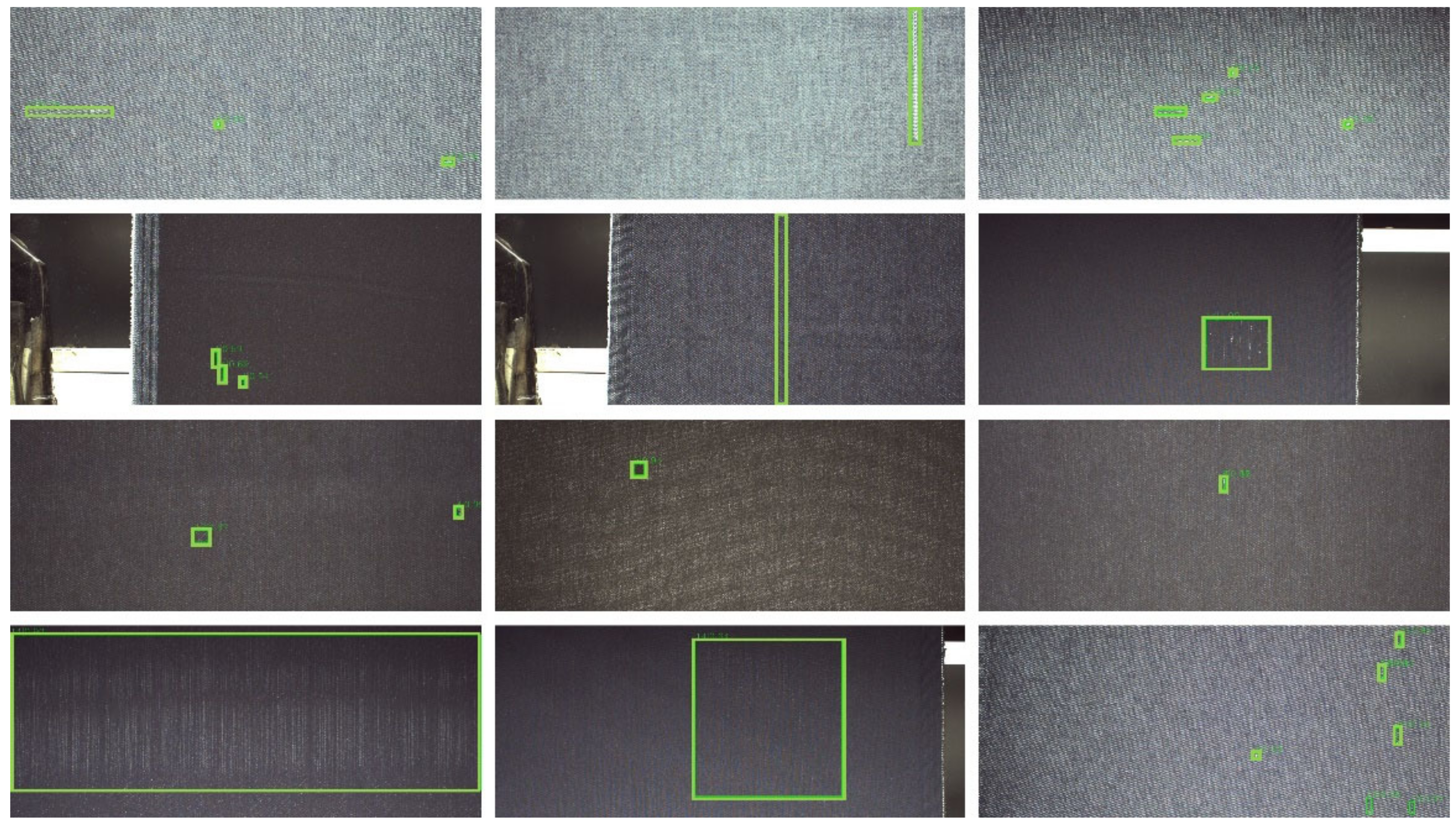
3.4. Detection Results

The proposed PRAN-Net based on Faster R-CNN in this paper was compared with RetinaNet, Mask R-CNN and Faster R-CNN with Guided Anchoring (GA-Faster R-CNN) on two fabric datasets, and all compared algorithms used ResNet-101-FPN [25] as backbone. The detection results were evaluated by ACC, AR, mAP, IoUs and FPS.

3.4.1. Detection Results of the Denim Dataset

The detection results by RetinaNet, Mask R-CNN, GA-Faster R-CNN and PRAN-Net are shown in Table 3. It can be seen that the inspection speed of RetinaNet is slightly faster than that of PRAN-Net, but the detection accuracy is much lower. Compared with Mask R-CNN, the ACC and the mAP of PRAN-Net have improved 2.5% and 3.9%, respectively, and the inspection speed is greatly improved. Compared with GA-Faster R-CNN, PRAN-Net also improves detection and position accuracy, while its detection speed is also faster than that of GA-Faster R-CNN.
The detection results by PRAN-Net for the denim dataset are shown in Figure 11.
To better present the location accuracy of defects by PRAN-Net, IoU examples of the detected defect and the GT boxes by RetinaNet, GA-Faster R-CNN and PRAN-Net are shown in Figure 12. (Mask R-CNN was not considered because its detection speed was too slow for online inspection.) The blue rectangles are the GT boxes of the defects, the yellow rectangles are the detected location corresponding to the defects and the green intersection regions are the IoU of the GT boxes with the detected defects of three methods, which are 55.1% for RetinaNet, 72.4% for GA-Faster R-CNN and 80.6% for PRAN-Net. Their IoU values are consistent with the tendency of IoUs as shown in Table 3, which are 63.8% for RetinaNet, 71.4% for GA-Faster R-CNN and 72.9% for PRAN-Net, respectively. All these indicate the better location precision of PRAN-Net for extreme shape defects.

3.4.2. Detection Results of the Plain Fabric Dataset

The test results of the plain fabric dataset with the four methods are also given in Table 4. It can be seen that PRAN-Net also has the obvious improvement with the plain fabric dataset. Furthermore, the detection results are better than that of the denim dataset because the defects of the plain fabric dataset are easier to distinguish from backgrounds. It should be highlighted that the FPS was improved more obviously than that of the denim dataset because the image size of the plain dataset is much smaller than that of the denim dataset. After the comprehensive comparison of the four methods, the detection performance on the plain fabric dataset of PRAN-Net is also the best.

4. Conclusions

This paper proposed a PRAN-Net method that improves the detection accuracy of fabric defects. Aiming at the problem that the initial anchor in the Faster R-CNN model is not suitable for tiny and extreme shape fabric defect detection, we propose Priori Anchor to effectively generate sparse anchors adaptively. On this basis, the FPN is used to obtain multi-scales feature maps to extract more detailed information of the defects. Two different fabric datasets were used to verify the performance of PRAN-Net by comparing it with RetinaNet, Mask R-CNN and GA-Faster R-CNN. Compared with the One-stage algorithm, the detection accuracy is improved 7.2% and 7.4% on the denim dataset and the plain fabric dataset separately, while the detection speed decreased less than 0.7f/s. Compared with the Two-stage algorithm, the mAP increases at least 2.1% and 2.4% separately on the two datasets. The PRAN-Net method increases detection and location accuracy for tiny and extreme fabric defects greatly, and the detection speed is also improved because of using fewer prior anchors, which satisfies the requirements of real-time detection. In the future, we will try PRAN-Net with other deep learning networks and apply to multiple tiny objects detection of other application fields.

Author Contributions

Conceptualization, methodology and software, P.P.; validation, P.P., Y.W. and C.H.; formal analysis, P.P. and Y.W.; investigation, P.P. and T.L.; resources, Z.Z. and W.Z.; writing—Original draft preparation, P.P.; writing—Review and editing, P.P. and Y.W.; funding acquisition, Y.W., Z.Z. and W.Z. All authors have read and agreed to the published version of the manuscript.

Funding

This research was funded by the Science Technology Service program of Science Academy of China under Grant KFJ-STS-QYZX-098 and the Strategic Priority Research Program of Science Academy of China under Grant XDA13030404.

Conflicts of Interest

The authors declare no conflict of interest.

References

  1. Sari-Sarra, H.; Goddard, J.S. Vision system for on-loom fabric inspection. IEEE Trans. Ind. Appl. 1999, 35, 1252–1259. [Google Scholar] [CrossRef]
  2. Dorrity, J.L.; Vachtsevanos, G. On-line defect detection for weaving systems. In Proceedings of the 1996 IEEE Annual Textile, Fiber and Film Industry Technical Conference, Atlanta, GA, USA, 15–16 May 1996; p. 6. [Google Scholar] [CrossRef]
  3. Chan, C.H.; Pang, G.K.H. Fabric defect detection by Fourier analysis. IEEE Trans. Ind. Appl. 2000, 36, 1267–1276. [Google Scholar] [CrossRef] [Green Version]
  4. Redmon, J.; Divvala, S.; Girshick, R.; Farhadi, A. You Only Look Once: Unified, Real-Time Object Detection. In Proceedings of the 2016 IEEE Conference on Computer Vision and Pattern Recognition (CVPR), Las Vegas, NV, USA, 27–30 June 2016; pp. 779–788. [Google Scholar] [CrossRef] [Green Version]
  5. Liu, W.; Anguelov, D.; Erhan, D.; Szegedy, C.; Reed, S.; Fu, C.-Y.; Berg, A.C. SSD: Single Shot MultiBox Detector. In Computer Vision—ECCV 2016; Springer: Cham, Switzerland, 2016; pp. 21–37. [Google Scholar] [CrossRef] [Green Version]
  6. Redmon, J.; Farhadi, A. YOLO9000: Better, Faster, Stronger. In Proceedings of the 2017 IEEE Conference on Computer Vision and Pattern Recognition (CVPR), Honolulu, HI, USA, 21–26 July 2017; pp. 6517–6525. [Google Scholar] [CrossRef] [Green Version]
  7. Lin, T.; Goyal, P.; Girshick, R.; He, K.; Dollár, P. Focal Loss for Dense Object Detection. In Proceedings of the 2017 IEEE International Conference on Computer Vision (ICCV), Venice, Italy, 22–29 October 2017; pp. 2999–3007. [Google Scholar] [CrossRef] [Green Version]
  8. Redmon, J.; Farhadi, A. YOLOv3: An Incremental Improvement. arXiv 2018, arXiv:1804.02767. Available online: https://arxiv.org/abs/1804.02767 (accessed on 8 April 2018).
  9. Bochkovskiy, A.; Wang, C.; Liao, H.M. YOLOv4: Optimal Speed and Accuracy of Object Detection. In Proceedings of the Conference on Computer Vision and Pattern Recognition (CVPR), USA, 16–18 June 2020. Virtual Online Meeting. [Google Scholar]
  10. Girshick, R.; Donahue, J.; Darrell, T.; Malik, J. Rich Feature Hierarchies for Accurate Object Detection and Semantic Segmentation. In Proceedings of the 2014 IEEE Conference on Computer Vision and Pattern Recognition, Columbus, OH, USA, 23–28 June 2014; pp. 580–587. [Google Scholar] [CrossRef] [Green Version]
  11. Girshick, R. Fast R-CNN. In Proceedings of the 2015 IEEE International Conference on Computer Vision (ICCV), Santiago, Chile, 7–13 December 2015; pp. 1440–1448. [Google Scholar]
  12. Dai, J.; Li, Y.; He, K.; Sun, J. R-FCN: Object Detection via Region-based Fully Convolutional Networks. In Advances in Neural Information Processing Systems 29; Curran Associates Inc.: Long Beach, CA, USA, 2016; pp. 379–387. [Google Scholar]
  13. Ren, S.; He, K.; Girshick, R.; Sun, J. Faster R-CNN: Towards Real-Time Object Detection with Region Proposal Networks. IEEE Trans. Pattern Anal. Mach. Intell. 2017, 39, 1137–1149. [Google Scholar] [CrossRef] [PubMed] [Green Version]
  14. He, K.; Gkioxari, G.; Dollár, P.; Girshick, R. Mask R-CNN. In Proceedings of the 2017 IEEE International Conference on Computer Vision (ICCV), Venice, Italy, 22–29 October 2017; pp. 2980–2988. [Google Scholar] [CrossRef]
  15. Cai, Z.; Vasconcelos, N. Cascade R-CNN: Delving Into High Quality Object Detection. In Proceedings of the 2018 IEEE/CVF Conference on Computer Vision and Pattern Recognition, Salt Lake City, UT, USA, 18–22 June 2018; pp. 6154–6162. [Google Scholar]
  16. Hu, Y.; Shan, Z.; Gao, F. Ship Detection Based on Faster-RCNN and Multiresolution SAR. Radio Eng. 2018, 48, 96–100. [Google Scholar]
  17. Jain, P.K.; Gupta, S.; Bhavsar, A.; Nigam, A.; Sharma, N. Localization of common carotid artery transverse section in B-mode ultrasound images using faster RCNN: A deep learning approach. Med. Biol. Eng. Comput. 2020, 58, 471–482. [Google Scholar] [CrossRef] [PubMed]
  18. Rosati, R.; Romeo, L.; Silvestri, S.; Marcheggiani, F.; Tiano, L.; Frontoni, E. Faster R-CNN approach for detection and quantification of DNA damage in comet assay images. Comput. Biol. Med. 2020, 123, 103912. [Google Scholar] [CrossRef] [PubMed]
  19. Liu, J.; Wang, C.; Su, H.; Du, B.; Tao, D. Multistage GAN for Fabric Defect Detection. IEEE Trans. Image Process. 2019, 29, 3388–3400. [Google Scholar] [CrossRef] [PubMed]
  20. Jing, J.; Ma, H.; Zhang, H. Automatic fabric defect detection using a deep convolutional neural network. Color. Technol. 2019, 135, 213–223. [Google Scholar] [CrossRef]
  21. Jing, J.; Zhuo, D.; Zhang, H.; Liang, Y.; Zheng, M. Fabric defect detection using the improved YOLOv3 model. J. Eng. Fibers Fabr. 2020, 15. [Google Scholar] [CrossRef] [Green Version]
  22. Lin, T.; Dollár, P.; Girshick, R.; He, K.; Hariharan, B.; Belongie, S. Feature Pyramid Networks for Object Detection. In Proceedings of the 2017 IEEE Conference on Computer Vision and Pattern Recognition (CVPR), Honolulu, HI, USA, 21–26 July 2017; pp. 936–944. [Google Scholar] [CrossRef] [Green Version]
  23. Zhou, X.Y.; Wang, D.; Krhenbühl, P. Objects as Points. arXiv 2019, arXiv:1904.07850v1. Available online: https://arxiv.org/abs/1904.07850v1 (accessed on 16 April 2020).
  24. Wang, J.; Chen, K.; Yang, S.; Loy, C.C.; Lin, D. Region Proposal by Guided Anchoring. In Proceedings of the 2019 IEEE/CVF Conference on Computer Vision and Pattern Recognition (CVPR), Long Beach, CA, USA, 15–20 June 2019; pp. 2960–2969. [Google Scholar] [CrossRef] [Green Version]
  25. He, K.; Zhang, X.; Ren, S.; Sun, J. Deep Residual Learning for Image Recognition. In Proceedings of the 2016 IEEE Conference on Computer Vision and Pattern Recognition (CVPR), Las Vegas, NV, USA, 27–30 June 2016; pp. 770–778. [Google Scholar] [CrossRef] [Green Version]
  26. Li, B.Y.; Liu, Y.; Wang, X. Gradient Harmonized Single-stage Detector. arXiv 2018, arXiv:1811.05181v1. [Google Scholar] [CrossRef]
  27. Everingham, M.; Van Gool, L.; Williams, C.K.I.; Winn, J.; Zisserman, A. The Pascal Visual Object Classes (VOC) Challenge. Int. J. Comput. Vis. 2010, 88, 303–338. [Google Scholar] [CrossRef] [Green Version]
Figure 1. The fabric defect detection process of the PRAN-Net.
Applsci 10 08434 g001
Figure 2. The schematic of features extraction in the PRAN-Net.
Applsci 10 08434 g002
Figure 3. The schematic of the priori anchor generation in the Priori Anchor Convolutional Neural Network (PRAN-Net).
Applsci 10 08434 g003
Figure 4. The architecture of the classification network in the PRAN-Net.
Applsci 10 08434 g004
Figure 5. Samples of the defects in the plain fabric images. (a) oil stain, (b) long coarse weft, (c) long coarse warp, (d) long coarse weft, (e) short coarse weft, and (f) mispick.
Applsci 10 08434 g005
Figure 6. The distribution of defects. (a) number of defects classes (b) defects aspect ratios.
Applsci 10 08434 g006
Figure 7. Defects of the denim fabric. (a) knot, (b) coarse warp, (c) three wire, and (d) flower jump.
Applsci 10 08434 g007
Figure 8. Intersection over union (IoU) of the detected defect and the ground truth. (a) the detected defect and the ground truth, and (b) the schematic of IoU.
Applsci 10 08434 g008
Figure 9. The definition of true positive (TP), false positive (FP), false negative (FN) and true negative (TN) of detected defects and true defects.
Applsci 10 08434 g009
Figure 10. The training loss value curves and accuracy curve of PRAN-Net for the denim dataset. (a) the total loss value curve, (b) the priori anchor loss value curve, (c) the classification network loss value curve and (d) the accuracy curve of the test set.
Applsci 10 08434 g010
Figure 11. The detection results of PRAN-Net for the denim dataset.
Applsci 10 08434 g011
Figure 12. The detected defects and their IoUs by three methods. (The blue boxes are the GT boxes, the yellow boxes are the correct detected boxes.) (a) the GT box in the fabric defect image, (b) the IoU of RetinaNet, (c) the IoU of GA-Faster R-CNN, and (d) the IoU of PRAN-Net.
Applsci 10 08434 g012
Table 1. The number of each category defect of the plain fabric dataset.
CategoryOil StainsCoarse WarpLong Coarse WeftShort Coarse WeftMispickTotal
Number of defectsTrain3914525230425765
Validation93662766189
Test1632648711210
Total64213378467421164
Table 2. Number of each category defects of the denim dataset.
CategoryFileStainsDifficultNepBroken WarpLight WarpLooped Weft
Defect Class Id1234567
Number of defectsTrain247265246133191104317
Validation61666133472679
Test53705929463056
Total361401361195284160452
CategoryStar JumpCoarse PickMispickStarch LumpWarp KnotBroken SpandexKnot
Defect Class Id891011121314
Number of defectsTrain2216561122433233661379
Validation5516427608091344
Test269522316789273
Total3029151613364735461996
Category NameFlower JumpCoarse WarpLoose WarpMarkThree WireHoleTotal
Defect Class Id151617181920
Number of defectsTrain961432673246981966527
Validation23356681174481621
Test15356365183681375
Total13421339647010553129523
Table 3. The detection results of the four methods with the denim dataset.
MethodThe Denim Dataset
ACC (%)mAP (%)AR (%)IoUs (%)FPS (f/s)
RetinaNet84.753.746.763.810.2
Mask R-CNN89.458.45169.80.3
GA-Faster R-CNN87.160.250.971.47.2
PRAN-Net91.962.353.372.99.7
Table 4. The detection results of the four methods with the plain fabric dataset.
MethodThe Plain Fabric Dataset
ACC (%)mAP (%)AR (%)IoUs (%)FPS (f/s)
RetinaNet91.283.753.688.726.1
Mask R-CNN96.490.166.693.10.8
GA-Faster R-CNN94.788.463.191.420.3
PRAN-Net98.692.570.095.825.4
Publisher’s Note: MDPI stays neutral with regard to jurisdictional claims in published maps and institutional affiliations.

