A Grey Wolf-Based Method for Mammographic Mass Classification

Abstract

Breast cancer is one of the most prevalent cancer types with a high mortality rate in women worldwide. This devastating cancer still represents a worldwide public health concern in terms of high morbidity and mortality rates. The diagnosis of breast abnormalities is challenging due to different types of tissues and textural variations in intensity. Hence, developing an accurate computer-aided system (CAD) is very important to distinguish normal from abnormal tissues and define the abnormal tissues as benign or malignant. The present study aims to enhance the accuracy of CAD systems and to reduce its computational complexity. This paper proposes a method for extracting a set of statistical features based on curvelet and wavelet sub-bands. Then the binary grey wolf optimizer (BGWO) is used as a feature selection technique aiming to choose the best set of features giving high performance. Using public dataset, Digital Database for Screening Mammography (DDSM), different experiments have been performed with and without using the BGWO algorithm. The random forest classifier with 10-fold cross-validation is used to achieve the classification task to evaluate the selected set of features’ capability. The obtained results showed that when the BGWO algorithm is used as a feature selection technique, only 30.7% of the total features can be used to detect whether a mammogram image is normal or abnormal with ROC area reaching 1.0 when the fusion of both curvelet and wavelet features were used. In addition, in case of diagnosing the mammogram images as benign or malignant, the results showed that using BGWO algorithm as a feature selection technique, only 38.5% of the total features can be used to do so with high ROC area result at 0.871.

1. Introduction

Breast cancer is affecting around 2.1 million women each year. It is the most frequent cancer among women and causes the highest number of cancer-related deaths [1]. In 2018, it was estimated that approximately 15% of all cancer deaths in women were due to breast cancer [2]. However, early detection is the key to decrease the death-rate. Screening programs using mammography images have proven to be the most powerful tool for breast cancer detection in its earlier stage [1,3]. A mammogram is an X-ray picture of the breast. The tumours have a high attenuation factor for X-rays. One limitation is when the breast tissue consists mainly of dense tissues, as the case with young women, and hence, challenges arise to detect these abnormalities. Therefore, an efficient method/system is still needed to detect and classify cancer from mammograms while reducing false positive and false negative ratios. Such method/system is important as a second reader to help the radiologists [4,5,6].

For mammogram analysis and classification, the multi-resolution analysis (MRA) approach [7] has been successfully used [8,9]. In the literature, Refs. [10,11,12] applied multi-resolution techniques to extract a set of different features. The mammographic images have been decomposed into several sub-bands. Curvelet and wavelet, as an efficient MRA, are used to analyse the original mammogram image in order to find out the features. In the literature, some authors selected the biggest coefficients [9], while others selected some statistical features of sub-bands [12]. On the other hand, some authors have combined the MRA features with the co-occurrence matrix features [10].

Eltoukhy et al. [13] used a set of features obtained using exact Gaussian–Hermite moments and employed three different classifiers. The successful employment of orthogonal moments encourage the authors to integrate three kinds of orthogonal moments in [14].

Pal [15] used a grey wolf optimization (GWO) algorithm to train feed foreword neural network (FFNN), which is then used for mammogram breast cancer classification. The proposed GWO-FFNN method showed promising results when evaluated using the Wisconsin Hospital Breast Cancer dataset. In addition, Mohanty et al. [16] have also applied the GWO algorithm to optimize the hidden node parameters of the extreme learning machine aiming to obtain a better performance of breast cancer detection. In another study [17], the GWO was combined with the decision tree to classify gene expression data. This combination was proposed to select a small set of genes from a group of genes to identify cancer.

In addition to employing GWO algorithm in breast cancer detection, it has been used as a feature selection technique in other applications in image processing. For example, it is used in the face recognition system [18]. GWO was used for feature selection, where k-Nearest Neighbour (KNN) was used for classification. The proposed method was estimated based on Yale face dataset. The obtained results showed better accuracy and run time compared to related work. In addition, Sreedharan et al. in [19], employed GWO as a feature selection technique for facial emotion recognition systems. They also used it along with neural network (NN) as a classifier for emotions from selected features. Comparing to conventional methods, NN-Levenberg–Marquardt (LM) and NN-particle swarm optimization (PSO), the accuracy of the obtained results was better than that of traditional methods.

In this paper, the proposed work intends to employ the BGWO as an efficient feature selection algorithm to select the most discriminative features that can distinguish between different mammographic image classes. The obtained feature vector is introduced to the random forest classifier to distinguish the normal mammographic image from the abnormal images in the first classification step. Secondly, to define the benign from the malignant region. A critical contribution of this work is to reduce the feature vector dimensionality. The computational complexity is scaled down, i.e., the feature vector length has been reduced to a small number of features, that will increase the speed of the extraction and matching processes. The random forest algorithm has the advantage of combining multiple weak classifiers using the method of ensemble learning. It can be used to enhance the prediction accuracy of unseen data. Its capabilities have been proven in mammographic mass detection [13,20].

The rest of this paper is constructed as follows: the preliminaries of the wavelet and curvelet are illustrated in Section 2. It is combined with a description of the statistical features applied in the study, grey wolf optimizer and random forest classifier. The suggested method is explained in Section 3. Section 4 presents the obtained results with an overview of the used dataset, evaluation criteria and a comparison with related work. Finally, the most important findings and conclusions are presented in Section 5.

2. Preliminaries

The present part shows an overview of the methods and algorithms employed in the suggested work. It highlights the wavelet, curvelet and grey wolf optimizer, and random forest classifier.

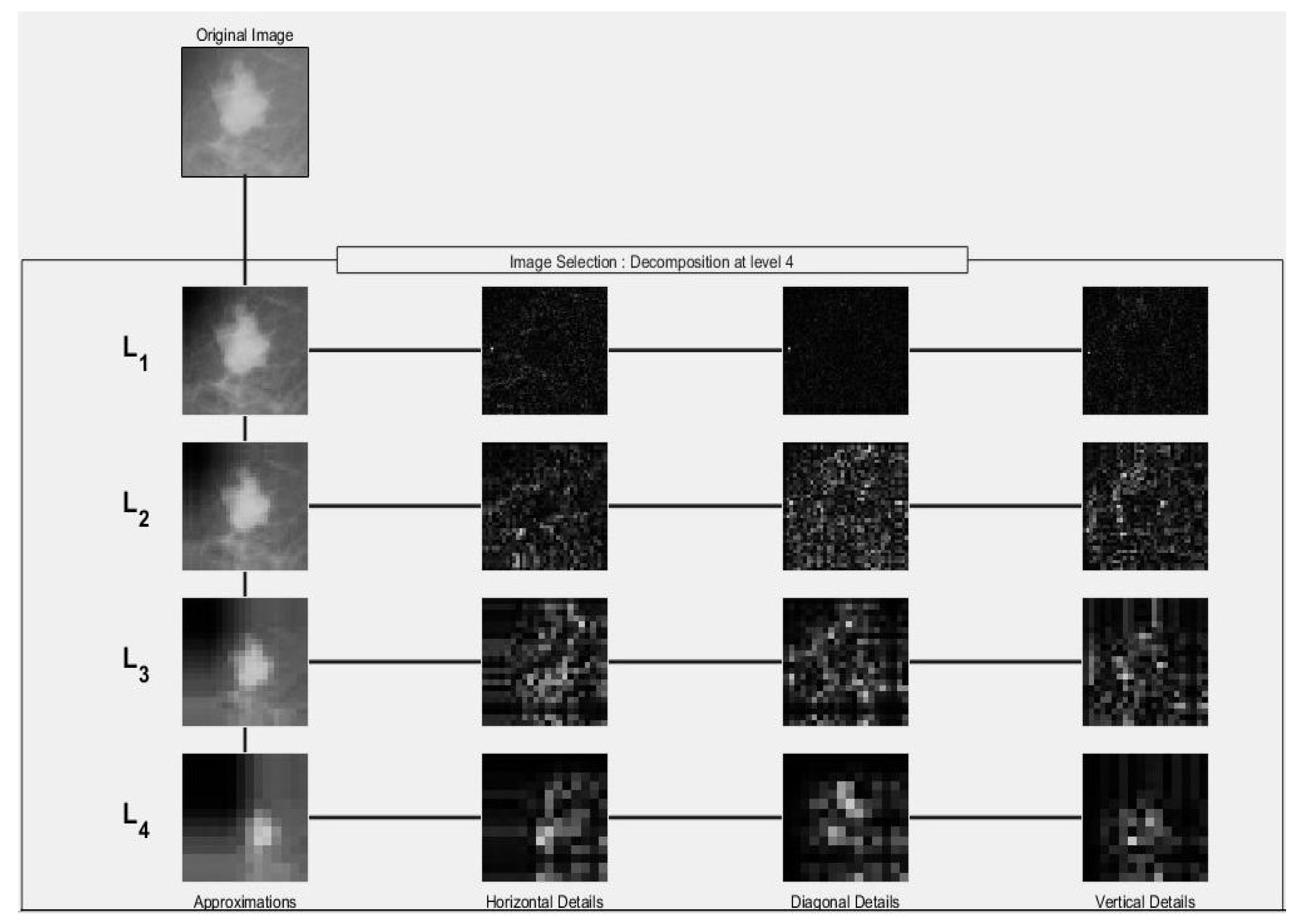
2.1. Wavelet Transform

Among the techniques for calculating the multi-resolution representation of signals, the wavelet transform technique is considered the most. This is because the wavelet transform technique enables the localization of information both in the time and frequency domain [21]. Equation (1) shows the formula for calculating the wavelet transform.

$${\Psi }_{a,b}=\frac{1}{\sqrt{\left|a\right|}}\Psi \left(\frac{x-b}{a}\right)$$

(1)

In Equation (1), b represents the location parameter, while a is used for scaling. The main idea of the wavelet transform is to approximately represent the signal using a set of basic mathematical functions. Equation (2) shows the wavelet transform of a function f(x) ∈ L²(R) as shown below:

$${\mathbf{C}}_f(a,b)=\frac{1}{\sqrt{\left|a\right|}}{\int }_{-\infty }^{\infty }f\left(x\right)\Psi \left(\frac{x-b}{a}\right)dx$$

(2)

In the equation, the function $f\left(x\right)$ is defined by its wavelet coefficients ${\mathbf{C}}_f(a,b),$ where $a>0$, b ∈ R. The discrete wavelet transform (DWT) is produced by taking $a=2^j,b=k{2}^j=ka$ for $k,j\in Z^2$.

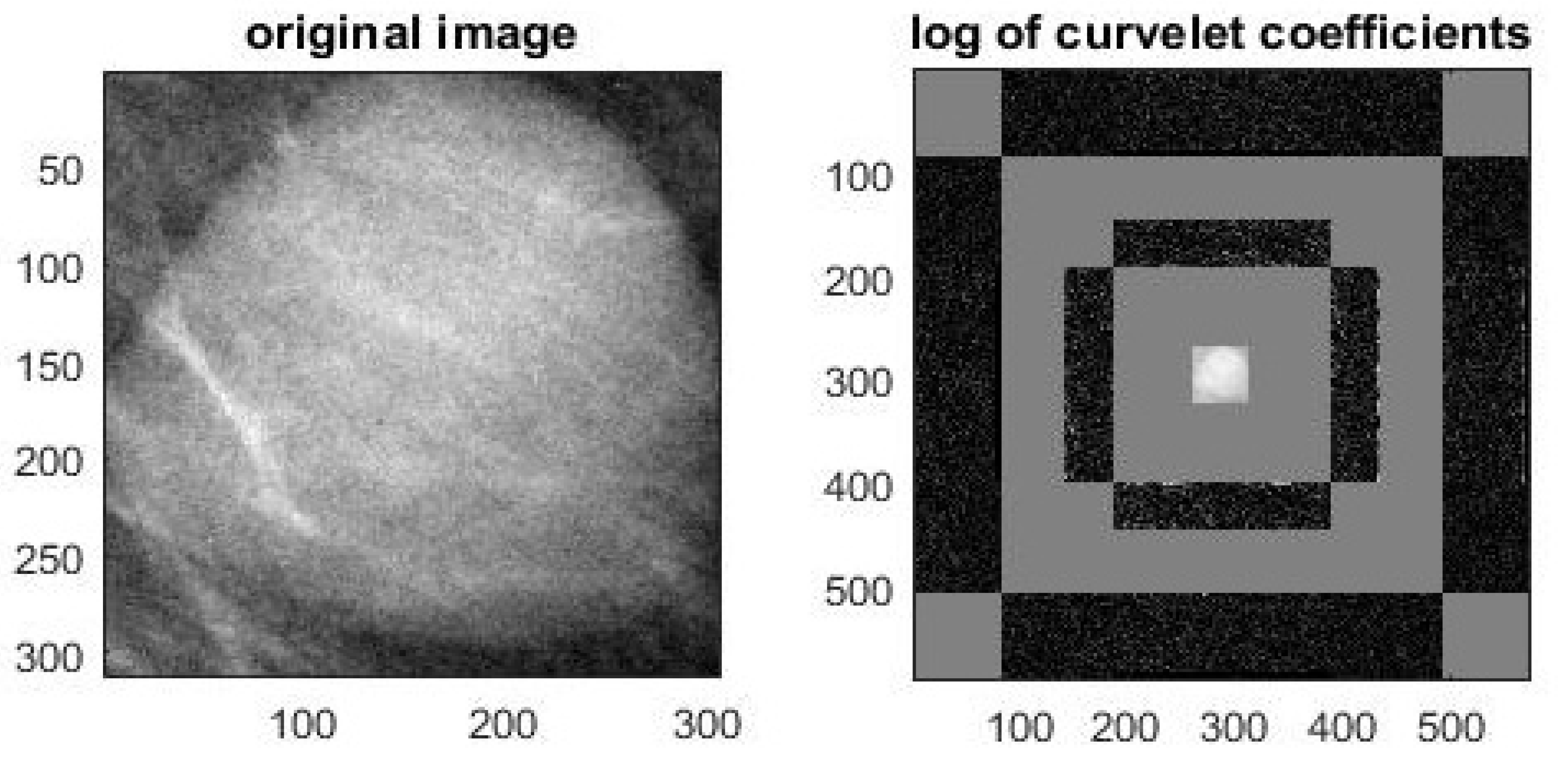
2.2. Curvelet Transform

A discrete curvelet transform is an approach used for representing images. This approach allows image codes to edge more efficiently. This is because of the geometric feature present in the curvelet transform approach. The coefficients produced from the discrete curvelet transform approach are used as a feature vector. Research conducted by [22] worked on A Fast Discrete Curvelet Transform (FDCT) approach. Since curvelets are stored in terms of vectors, the research uses two dimensions for storing features. These include $R^2$ with x as a spatial variable, $\omega$ as frequency domain variable, r and $\theta$ polar coordinates in the frequency domain. $W\left(r\right)$ and $V\left(t\right),$ which are a pair of windows, are also defined. They are used as radial and angular windows, respectively. All vectors are smooth, positive and real values, where W uses non-negative real arguments and supported on $r\in (1/2,2)$ and V uses real arguments and supported on $t\in [-1,1].$ Both windows $W\left(r\right)$ and $V\left(t\right)$ follow the admissibility conditions defined by [21]. Equations (3) and (4) shows formulae for these windows, as shown below:

$$\sum _{j=-\infty }^{\infty }{W}^2\left(2^{j}r\right)=1,r\in \left(\frac{3}{4},\frac{3}{2}\right)$$

(3)

$$\sum _{l=-\infty }^{\infty }{V}^2(t-l)=1,t\in \left(-\frac{1}{2},\frac{1}{2}\right)$$

(4)

For each $j\ge j_0$, a frequency window $U_j$ is defined in the Fourier domain by

$$U_j(r,\theta )=2^{-\frac{3}{4}j}W\left(2^{-j}r\right)V\left(\frac{2^{⌊\frac{j}{2}⌋}\theta }{2\pi }\right)$$

(5)

In Equation (5), $\lfloor j/2\rfloor$ is used as an integer. Moreover, $U_j$ is used as a polar wedge which is calculated using the results from the radial and angular windows W and V. To obtain real-valued curvelets, the symmetrized version of Equation (5) can be obtained using $U_j(r,\theta )+U_j(r,\theta +\pi )$.

Similarly, the waveform ${\phi }_j\left(x\right)$ can be defined using Fourier transform $\widetilde{{\phi }_j}\left(\omega \right)=U_j\left(\omega \right)$ as shown in Equation (6). Using Equation (5), we can obtain $U_j\left({\omega }_1,{\omega }_2\right),$ where ${\omega }_1,{\omega }_2$ are the windows defined in the polar coordinate system. In Equation (6), ${\phi }_j$ is used as the major curvelet which encapsulates all curvelets at scale $2^{-j}$ that are obtainable using rotations and translations of ${\phi }_j.$ Here, we introduce rotation angles ${\theta }_l=2\pi ·2^{-\lfloor j/2\rfloor }·l,$ with $l=0,1,\dots$ such that $0\le \theta \le 2\pi$. Moreover, $k=\left(k_1,k_2\right)\in {\mathrm{Z}}^2,$ which identifies the sequence of translation parameters. The curvelets are defined (as a function of $x=\left(x_1,x_2\right)$) at scale $2^{-j},$ orientation angle ${\theta }_l$ and position $x_k^{(j,l)}=$ $R_{{\theta }_l}^{-1}\left(k_1·2^{-j},k_2·2^{-j/2}\right)$ by

$${\phi }_{j,l,k}\left(x\right)={\phi }_j\left(R_{{\theta }_l}\left(x-x_k^{(j,l)}\right)\right)$$

(6)

where $R_{\theta }$ is the rotation by $\theta$ radians and $R_{\theta }^{-1}$ its inverse,

$${\mathrm{R}}_{\theta }=\left(\begin{array}{cc}cos\theta & sin\theta \\ -sin\theta & cos\theta \end{array}\right),{\mathrm{R}}_{\theta }^{-1}={\mathrm{R}}_{\theta }^{\mathrm{T}}={\mathrm{R}}_{-\theta }$$

The inner product between an element $f\in L^2\left({\mathbf{R}}^2\right)$ and a curvelet ${\phi }_{j,l,k},$ is defined as a curvelet coefficient.

$$c(j,l,k):={\int }_{{\mathbf{R}}^2}^{}f\left(x\right)\overline{{\phi }_{j.l.k}\left(x\right)}dx$$

(7)

where R denotes the real line. Length ≈$2^{-j/2},$ width $=2^{-j}$, i.e., width ≈ length ${}^2$ which is known as a curve scaling law or anisotrpoy scaling relation [23].

2.3. Feature Extraction: Statistical Features of Wavelet and Curvelet

In this paper, the coefficients in each sub-band of both wavelet and curvelet will be described by ten descriptors/features which are presented as follow. These features are produced according to grey level distribution across the image. In our proposed method, the ten features are statistical ones which are formally described below [24].

Mean: for a collection of numeric data, $x_1,x_2,\dots ,x_n$, the sample mean is the numerical average [25]:

$$\overline{x}=\frac{1}{n}\left(x_1+x_2+\dots +x_n\right)=\frac{1}{n}\sum _{i=1}^n{x}_i$$

(8)

The variance is a measure that shows the width of the histogram. It determines how much the grey levels differ from their mean. The variance gives a sense of the spread of the values of a random variable. The variance averages the square of the differences from the mean. The square root of the variance is knowen as the standard deviation [25].

$$Var=\frac{1}{\mathrm{n}-1}\sum {(\mathrm{P}[\mathrm{i},\mathrm{j}]-\overline{\mathrm{P}}[\mathrm{i},\mathrm{j}])}^2$$

(9)

$$STD=\sqrt{\frac{1}{\mathrm{n}-1}\sum {(\mathrm{P}[\mathrm{i},\mathrm{j}]-\overline{\mathrm{P}}[\mathrm{i},\mathrm{j}])}^2}$$

(10)

The third moment of the standardized random variable is called the skewness. Skewness ${\mu }_3$ is used to measure the degree of histogram asymmetry around the mean. At the same time, kurtosis ${\mu }_4$ is used to measure the sharpness of the histogram. Significant skewness and kurtosis indicate that data are not normal [24,26]. Skewness and kurtosis are defined as in Equations (11) and (12):

$$S=E\left[{\left(\frac{X-\mu }{\sigma }\right)}^3\right]$$

(11)

$$K=E\left[{\left(\frac{X-\mu }{\sigma }\right)}^4\right]$$

(12)

Energy can be calculated as follows [25]:

$$Energy=\sum _{\mathrm{i}}^{\mathrm{M}}\sum _{\mathrm{j}}^{\mathrm{N}}{\mathrm{P}}^2[\mathrm{i},\mathrm{j}]$$

(13)

The entropy is used to measure the randomness of an image. It is low for the smooth images and high for the rough images. The entropy is calculated by [25]:

$$Entropy=-\sum _i^M\sum _j^{N}P[i,j]logP[i,j]$$

(14)

The maximum value is defined as the highest value in the given matrix. It is calculated as follow:

$$\begin{array}{c}M,N\hfill \\ Max=maxP[i,j]\hfill \\ i,j\hfill \end{array}$$

(15)

Homogeneity is used as a measure of similarity of the distribution of elements in the grey levels. Its value varies between 0 and 1. If the value is close to one, it means a smoother texture image, and so on. Mathematically, homogeneity of an image is defined as [24]:

$$Homogeneity=\sum _i^M\sum _j^N\frac{1}{1+{(i-j)}^2}·P(i,j)$$

(16)

Moment is employed as a global feature of an image that is widely used in pattern recognition and image classification [24].

$$moment=\sum _i^M\sum _j^N\frac{P(i,j)}{{(i-j)}^2}$$

(17)

2.4. Feature Selection: Binary Grey Wolf Optimizer

Mirjalili et al. [27] proposed a metaheuristic optimization method namely grey wolf optimizer (GWO). The name is given because the algorithm follows the hunting method and leadership pyramid seen in grey wolves. The size of a grey wolves’ pack is usually between 5 to 12, where the population is divided into ranks of Alpha, Beta, Delta and Omega. In this distribution, alpha is considered the leader of the pack. The Alpha makes all the important decision making for the pack. Moving down the chain, the Beta wolf assists the alpha wolf in decision making and other matters. Delta wolves are known as subordinate wolves, which work directly under Alpha and Beta wolves, but have dominance over Omega wolves. They help the pack by protecting them and following orders given by Alpha and Beta wolves. Omega wolves are considered as a scapegoat or the expendables of the pack. However, they play an essential role in providing and performing scouting, alerting regarding danger and protecting the pack from foreigners. The notations used for Alpha, Beta, Delta and Omega are $\alpha ,\beta ,\gamma$ and $\omega$, respectively. This work employed the competitive binary grey wolf optimizer presented in Ref [28].

2.5. Classification: Random Forests

Random forests [29] is an ensemble learning method for supervised machine learning. The ensemble concept of random forest meaning that combining multiple weak classifiers could produce an accurate classification rate. Random forest combined results of multiple decision trees to enhance the prediction accuracy. In this study, the classification step has been performed employing 10-fold cross-validation to test the accuracy of the proposed method.

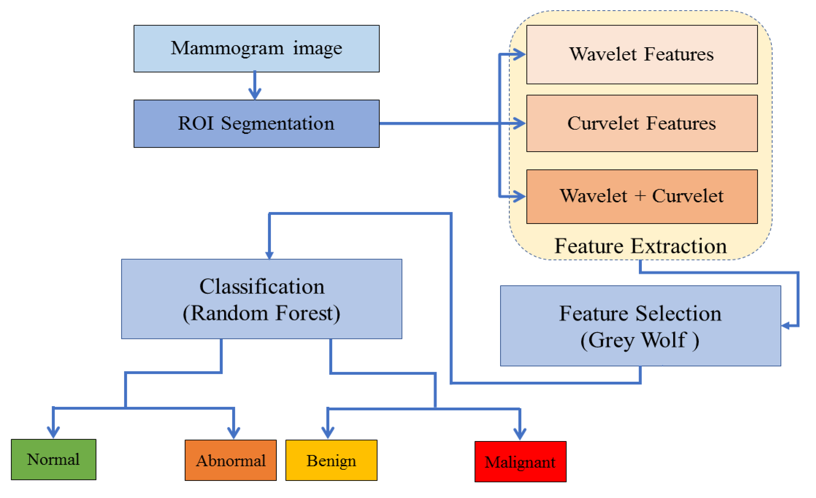
3. The Proposed Method

The proposed method, as explained in Figure 1, consists of four phases: Region of interest (ROI) segmentation, feature extraction, feature selection and classification.

In phase 1, the ROI is manually segmented in a way that the given centre of abnormality is the centre of the cropped ROI. In phase 2, features are extracted using wavelet and curvelet. Using a concatenation method, a fusion of wavelet and curvelet features are constructed. This gave three types of features: wavelet, curvelet and fused wavelet and curvelet features.

The curvelet and wavelet transform have proved their capability to represent the image in the frequency domain accurately. It decomposed the ROI into several sub-bands. The statistical features described in Section 2.3 are calculated for each sub-band to construct the feature vectors. In this study, we have the following three scenarios.

The first one is to compute the ten features from the curvelet sub-bands (i.e., wedge). In order to achieve this task, the curvelet transform is applied to ROI, as shown in Figure 2. The ten features (described above) for each wedge are calculated using Equations (8)–(17). In this work, the curvelet is applied using four scales with 16 angles. Hence, the curvelet decomposition produced 81 wedges, so a total of 810 features are calculated to construct a features vector of the curvelet.

The second scenario is to employ the wavelet decomposition of 16 bands to extract each band’s ten features. This is accomplished as follows. Daubechies 4 (DB4) wavelet is proved to be efficient as reported in [6]. This is why it was used in our proposed method to decompose the ROI image into four levels. Each of these levels composes of four sub-bands: approximation (A), horizontal (H), vertical (V) and diagonal (D). Hence, a total of 16 sub-bands can be obtained, see Figure 3. For each sub-band, the ten features are calculated. Therefore, a total of 160 features will be extracted from each ROI (i.e., 16 sub-bands × 10 Features) producing the wavelet feature vector.

The third scenario is to fuse the feature vector of both the curvelet and the wavelet. This produced a feature vector with length (810 + 160 = 970 features). The obtained feature vectors could improve the classification rate of mammographic images.

In phase 3, the BGWO algorithm, described in Section 2.4, is applied to select the best set of features given the best performance which is measured in the classification phase (i.e., phase 4). In this phase, the random forest, introduced earlier in Section 2.5, has been used to classify the selected features into normal or abnormal. The same set of features is also used to differentiate between benign or malignant cases.

4. Experimental Results

The proposed method is applied to the DDSM dataset. The following subsection presents an overview of the used DDSM dataset.

4.1. Mammography Dataset (DDSM)

To assess the proposed method, we used the DDSM public dataset which is considered the largest mammography dataset [30]. The dataset was collected by a research team at the University of South Florida. It consists of 2620 patients classified into 43 different volumes with each patient having four mammograms. Each mammogram is taken from two different views: Mediolateral oblique view (MLO) and craniocaudal (CC). The average size of the mammograms is (3000 × 4800) pixels and each mammogram has its ground truth information specified by experts, showing whether the image is benign or malignant as well as the lesion localization [30]. Using the breast imaging-reporting and data system (BI-RAD) scores, the DDSM database is classified by experts into three classes: normal, benign and malignant [30].

The dataset used to test the proposed method consists of 400 ROIs. A total of 200 ROIs are normal breast parenchyma and 200 ROIs are masses which are further classified into two sub-classes (100 benign and 100 malignant). A sample of the used dataset is illustrated in

Table 1. The used ROI datasets for proposed method assessment.

Dataset	Abnormal ROI		Normal ROI
	Benign	Malignant
Detection (Normal-Abnormal)	100	100	200
Diagnosis (Benign-Malignant)	100	100	-

. A sample of the DDSM regions used in the study is shown in Figure 4.

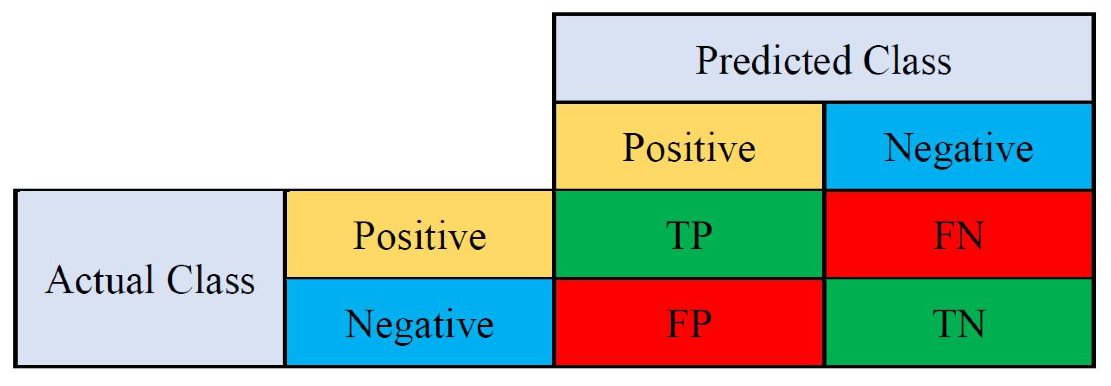
4.2. Evaluation Criteria

To assess the results of the proposed method, a set of popular benchmark metrics have been applied. Considering the confusion matrix obtained from the classification step, as shown in Figure 5, the following metric are used and they are briefly highlight as follows:

Accuracy: This is to show percentage of correctly predicted classes to the total number of classes. It can be calculated as follows:

$$Accuracy=\frac{TP+TN}{TP+TN+FP+FN}$$

Precision: This is show the percentage of correctly positive predicted classes to the total positive predicted classes. A high precision confirms a low FP rate.

$$Precision=\frac{TP}{TP+FP}$$

Recall (Sensitivity): This is show the percentage of correctly positive predicted samples to all samples in an actual class. A high recall confirms a low FN rate.

$$Recall=\frac{TP}{TP+FN}$$

The area under the ROC (Receiver Operating Characteristics) curve is a graph of two-dimensional plot: sensitivity versus specificity. This curve is considered one of the important factors for evaluating the performance of classification systems where value 1.0 reflects that the system has a perfect performance.

4.3. Results and Discussion

As presented in Figure 1, there are two variants of our method. One aims to classify ROI images into normal and abnormal, i.e., detecting abnormal breast cases. The second variant is to detect benign or malignant cases from the ROI images directly, i.e., diagnosing whether an ROI image is benign or malignant. It is notable that the features used in both variants are the same, but the type of features would be different based on the BGWO selection. There are two main scenarios (without using BGWO and with using BGWO) in which the random forest algorithm is used to achieve the classification task.

Without using BGWO as a feature selection technique: The first scenario is designed to understand the performance of the feature sets (curvelet, wavelet and combining both curvelet and wavelet) without using the BGWO algorithm as a feature selection technique. The summary of the results of this scenario is shown in

Table 2. The classification performance without applying the binary grey wolf optimizer (BGWO).

	Selected Features	Number of Features	Accuracy	Precision	Recall	ROC Area
Normal vs. Abnormal	Curvelet	810	97.5%	97.5%	97.5%	0.995
	Wavelet	160	98.3%	98.3%	98.3%	0.998
	Curvelet + Wavelet	970	99.0%	99.0%	99.0%	1.00
Benign vs. Malignant	Curvelet	810	74.0%	74.2%	74.0%	0.863
	Wavelet	160	73.0%	73.2%	73.0%	0.873
	Curvelet + Wavelet	970	74.0%	74.1%	74.0%	0.871

. From the obtained results, the following notes can be mentioned. Firstly, in case of detecting normal or abnormal cases, the best results are achieved when the fusion of both curvelet and wavelet was used with accuracy 99.0%, precision 99.0%, recall 99.0% and ROC area 1.00. These results would make sense as the fused features contain the most discriminative features from each of the wavelet and curvelet. Secondly, in case of diagnosing a raw ROI image, whether it is a benign or malignant case, the fused features and curvelet-based features gave the best results with very close performance in terms of accuracy 74.0%, precision 74.0%, recall 74.0% and ROC area 0.871. The main difference between used features and curvelet-based features is the number of features where the curvelet only needed 810 instead of 970 for the fused one. However, the results of the second scenario are not as good as in detecting normal or abnormal cases.

With using BGWO as a feature selection technique: In the second scenario, as in the first one, the same feature sets (i.e., the main features of curvelet (810), wavelet (160) and fused curvelet with wavelet (970)) will be fed to the BGWO algorithm to select the best feature set that would discriminate between different classes (normal, abnormal, benign or malignant).

This scenario is further divided into different sub-scenarios based on the feature type as shown below. Before describing the results of these two scenarios, it is worth mentioning that BGWO algorithm is a stochastic technique. Mittal et al. [31] reported that the stochastic algorithms need to be run at least 10 times to produce meaningful results. Usually, the average of these results is used to report the performance of these types of heuristic algorithms. In this paper, we followed the same approach where the proposed BGWO-based method was run 20 times with each run, one set of features was produced and then fed to the classifier (random forest) to evaluate whether this set would give the best results in terms of accuracy, precision, recall and ROC.

Table 3. Detection of normal or abnormal using BGWO with curvelet features.

Selected Features	Number of Features	Accuracy	Precision	Recall	ROC Area
Feat. set 1	250	93.8%	94.0%	93.8%	0.984
Feat. set 2	222	97.8%	97.8%	97.8%	0.997
Feat. set 3	241	95.8%	95.8%	95.8%	0.991
Feat. set 4	224	97.5%	97.5%	97.5%	0.996
Feat. set 5	264	95.0%	95.5%	95.0%	0.993
Feat. set 6	207	97.5%	97.6%	97.5%	0.999
Feat. set 7	251	98.3%	98.3%	98.2%	0.998
Feat. set 8	262	97.0%	97.0%	97.0%	0.995
Feat. set 9	258	94.3%	94.4%	94.3%	0.986
Feat. set 10	277	98.0%	98.0%	98.0%	0.999
Feat. set 11	294	94.8%	95.0%	94.8%	0.986
Feat. set 12	307	96.3%	96.3%	96.3%	0.99
Feat. set 13	188	97.0%	97.0%	97.0%	0.998
Feat. set 14	229	97.8%	97.8%	97.8%	0.999
Feat. set 15	275	98.0%	98.0%	98.0%	0.999
Feat. set 16	330	96.5%	96.7%	96.5%	0.995
Feat. set 17	296	97.5%	97.5%	97.5%	0.998
Feat. set 18	311	96.0%	96.2%	96.0%	0.99
Feat. set 19	194	98.0%	98.0%	98.0%	0.998
Feat. set 20	265	95.3%	95.4%	95.3%	0.995

,

Table 4. Detection of normal or abnormal using BGWO with wavelet features.

Selected Features	Number of Features	Accuracy	Precision	Recall	ROC Area
Feat. set 1	56	98.0%	98.0%	98.0%	0.995
Feat. set 2	49	96.8%	96.8%	96.8%	0.996
Feat. set 3	50	96.0%	96.0%	96.0%	0.992
Feat. set 4	62	97.3%	97.3%	97.3%	0.995
Feat. set 5	67	96.3%	96.3%	96.3%	0.995
Feat. set 6	40	98.0%	98.1%	98.0%	0.997
Feat. set 7	54	98.5%	98.5%	98.5%	0.997
Feat. set 8	90	98.3%	98.3%	98.3%	0.997
Feat. set 9	62	97.8%	97.8%	97.8%	0.998
Feat. set 10	42	98.8%	98.8%	98.8%	0.998
Feat. set 11	42	96.8%	96.8%	96.8%	0.994
Feat. set 12	46	99.0%	99.0%	99.0%	0.999
Feat. set 13	49	97.8%	97.8%	97.8%	0.997
Feat. set 14	65	98.8%	98.8%	98.8%	0.998
Feat. set 15	55	95.8%	95.8%	95.8%	0.991
Feat. set 16	51	96.0%	96.0%	96.0%	0.995
Feat. set 17	52	98.5%	98.5%	98.5%	0.997
Feat. set 18	56	97.0%	97.0%	97.0%	0.997
Feat. set 19	54	97.3%	97.3%	97.3%	0.992
Feat. set 20	55	99.0%	99.0%	99.0%	0.998

,

Table 5. Detection of normal or abnormal using BGWO with the fusion of curvelet and wavelet features.

Selected Features	Number of Features	Accuracy	Precision	Recall	ROC Area
Feat. set 1	279	96.8%	96.8%	93.6%	0.994
Feat. set 2	270	98.5%	98.5%	97.0%	0.997
Feat. set 3	350	98.0%	98.0%	96.0%	0.998
Feat. set 4	336	97.5%	97.6%	95.1%	0.999
Feat. set 5	273	97.8%	97.8%	95.6%	0.998
Feat. set 6	318	97.8%	97.8%	95.5%	0.998
Feat. set 7	246	98.8%	98.8%	97.5%	0.999
Feat. set 8	375	98.8%	98.8%	97.5%	1.0
Feat. set 9	399	98.5%	98.5%	97.0%	0.998
Feat. set 10	408	98.8%	98.8%	97.5%	0.999
Feat. set 11	337	99.0%	99.0%	98.0%	1.0
Feat. set 12	301	97.0%	97.0%	94.0%	0.996
Feat. set 13	273	99.3%	99.3%	98.5%	0.999
Feat. set 14	269	97.0%	97.0%	94.0%	0.995
Feat. set 15	298	100%	100%	100%	1.0
Feat. set 16	333	98.3%	98.3%	96.5%	0.998
Feat. set 17	246	99.5%	99.5%	99.0%	1.0
Feat. set 18	349	97.8%	97.8%	95.5%	0.997
Feat. set 19	259	97.5%	97.5%	95.0%	0.996
Feat. set 20	281	98.3%	98.3%	96.5%	1.0

,

Table 6. Detection of benign or malignant using BGWO with curvelet features.

Selected Features	Number of Features	Accuracy	Precision	Recall	ROC Area
Feat. set 1	313	71.5%	71.5%	71.5%	0.854
Feat. set 2	254	72.5%	72.6%	72.5%	0.851
Feat. set 3	275	72.5%	72.7%	72.5%	0.863
Feat. set 4	331	73.5%	73.7%	73.5%	0.875
Feat. set 5	279	72.5%	72.7%	72.5%	0.861
Feat. set 6	346	72.5%	72.6%	72.5%	0.855
Feat. set 7	268	69.0%	69.3%	69.0%	0.847
Feat. set 8	287	72.5%	72.9%	72.5%	0.857
Feat. set 9	266	72.0%	72.1%	72.0%	0.861
Feat. set 10	259	72.5%	72.5%	72.5%	0.856
Feat. set 11	266	72.5%	72.7%	72.5%	0.857
Feat. set 12	305	72.0%	72.0%	72.0%	0.855
Feat. set 13	315	70.5%	70.5%	70.5%	0.855
Feat. set 14	232	74.5%	74.7%	74.5%	0.858
Feat. set 15	246	71.0%	71.4%	71.0%	0.85
Feat. set 16	305	77.0%	77.0%	77.0%	0.87
Feat. set 17	315	74.5%	74.7%	74.5%	0.859
Feat. set 18	336	72.5%	72.5%	72.5%	0.863
Feat. set 19	268	72.0%	72.3%	72.0%	0.862
Feat. set 20	305	76.0%	76.0%	76.0%	0.872

,

Table 7. Detection of benign or malignant using BGWO with wavelet features.

Selected Features	Number of Features	Accuracy	Precision	Recall	ROC Area
Feat. set 1	67	75.0%	75.3%	75.0%	0.868
Feat. set 2	74	72.0%	72.2%	72.0%	0.857
Feat. set 3	60	74.5%	74.9%	74.5%	0.872
Feat. set 4	67	77.5%	77.7%	77.5%	0.891
Feat. set 5	56	77.0%	77.4%	77.0%	0.868
Feat. set 6	55	74.5%	74.8%	74.5%	0.875
Feat. set 7	70	74.5%	74.7%	74.5%	0.867
Feat. set 8	71	74.0%	74.6%	74.0%	0.864
Feat. set 9	54	74.5%	74.9%	74.5%	0.863
Feat. set 10	44	76.0%	76.3%	76.0%	0.869
Feat. set 11	61	75.5%	75.9%	75.5%	0.868
Feat. set 12	60	77.5%	77.8%	77.5%	0.886
Feat. set 13	75	75.0%	75.1%	75.0%	0.882
Feat. set 14	44	76.5%	77.3%	76.5%	0.867
Feat. set 15	59	74.0%	74.0%	74.0%	0.849
Feat. set 16	54	75.0%	75.1%	75.0%	0.871
Feat. set 17	59	72.5%	72.8%	72.5%	0.863
Feat. set 18	92	75.0%	75.4%	75.0%	0.882
Feat. set 19	62	73.5%	73.7%	73.5%	0.862
Feat. set 20	54	74.5%	74.9%	74.5%	0.872

and

Table 8. Detection of benign or malignant using BGWO with fusion features of curvelet and wavelet.

Selected Features	Number of Features	Accuracy	Precision	Recall	ROC Area
Feat. set 1	365	73.0%	73.0%	73.0%	0.856
Feat. set 2	319	75.0%	75.1%	75.0%	0.87
Feat. set 3	409	72.0%	72.0%	72.0%	0.85
Feat. set 4	354	72.5%	72.6%	72.5%	0.85
Feat. set 5	367	76.5%	76.6%	76.5%	0.86
Feat. set 6	374	78.0%	78.1%	78.0%	0.871
Feat. set 7	304	74.5%	74.6%	74.5%	0.871
Feat. set 8	374	74.5%	74.6%	74.5%	0.865
Feat. set 9	418	77.5%	77.6%	77.5%	0.88
Feat. set 10	396	72.5%	72.7%	72.5%	0.859
Feat. set 11	388	77.5%	76.6%	76.5%	0.86
Feat. set 12	305	74.5%	74.5%	74.5%	0.865
Feat. set 13	351	73.5%	73.8%	73.5%	0.864
Feat. set 14	312	73.0%	73.5%	73.0%	0.871
Feat. set 15	303	72.5%	72.7%	72.5%	0.867
Feat. set 16	345	70.0%	70.2%	70.0%	0.851
Feat. set 17	405	72.5%	72.6%	72.5%	0.86
Feat. set 18	356	72.0%	72.2%	72.0%	0.865
Feat. set 19	365	73.0%	73.2%	73.0%	0.861
Feat. set 20	340	74.0%	74.5%	74.0%	0.872

present a summary of these results where the best result of these 20 sets is highlighted in each table. Specifically, Table 3, Table 4 and Table 5 summarize the results of using BGWO to detect normal or abnormal cases while Table 6, Table 7 and Table 8 summarize the results of using BGWO to detect benign and malignant cases.

BGWO for normal and abnormal cases: To classify images into normal and abnormal, this scenario aims to check which features (curvelet, wavelet and combining both curvelet and wavelet) can be selected using BGWO algorithm to give the highest classification measures. The results of this scenario can be summarized as follows.

1

When the 810 curvelet features were used, Set 15 gave the best results with the number of features being 275, accuracy 98.0%, precision 98.0%, recall 98.0% and ROC area 0.999, see Table 3.

2

When the 160 wavelet features were used, Set 12 gave the best results with the number of features being 46, accuracy 99.0%, precision 99.0%, recall 99.0% and ROC area 0.999, see Table 4.

3

When the 970 fusion of both curvelet and wavelet features were used, Set 15 gave the best results with the number of features being 298, accuracy 100%, precision 100%, recall 100% and ROC area 1.00, see Table 5.

From the above three sub-scenarios, it can be noticed that the BGWO algorithm worked very well with the fused features where it has a big impact of the features reduction (i.e., 298 out of 970 were selected to give the highest results). The BGWO as a feature selector with fused curvelet and wavelet features gave the best results in terms of accuracy, precision, recall and ROC area among all the results of other features i.e., wavelet and curvelet individually. This means that if the BGWO algorithm is used as a feature selection technique, only 30.7% of the total mammogram features can be used to detect whether a mammogram image is normal or abnormal.

When comparing the results in Table 2 and in Table 3, Table 4 and Table 5, i.e., without and with using BGWO as a feature selection technique, respectively, it can be noticed that the use of BGWO has improved the results of all scenarios. In case of using the curvelet only, the results have improved by 0.5% for all evaluation measures while the needed features have been reduced from 810 to 275. In case of using the wavelet only, the results have also improved by 0.7% for accuracy, precision and recall and by 0.001 for the ROC area while the used features were reduced from 160 to 46 (this is a big improvement in terms of performance). For the last scenarios, i.e, when using fused curvelet and wavelet features, the results of using BGWO showed an improvement of 1.0% for accuracy, precision and recall and giving the same results (1.00) for the ROC area. This was achieved while only using 298 out of 970 features. Thus, it can be claimed that using BGWO could improve the detection of abnormal mammogram cases in terms of the processing requirements (i.e., using small size of features) and the performance requirements (i.e., accuracy, precision, recall and the ROC area).

Using BGWO for benign and malignant cases: This scenario aims to classify mammogram images as benign and malignant directly, i.e., helping in the cancer diagnosis process. In other words, it investigates which set of features would give high classification (benign and malignant) performance.

1

When the curvelet features (810 features) were given to the BGWO algorithm, the best result was obtained by Set 16 with a number of features 305, accuracy 77%, precision 77%, recall 77% and ROC area 0.87, see Table 6.

2

When the wavelet features, 160 features, were fed to the BGWO algorithm, the results showed that Set 4 gave the best results with the number of features being 67, accuracy 77.5%, precision 77.7%, recall 77.5% and ROC area 0.891, see Table 7.

3

When the fused features of both curvelet and wavelet features, 970 features, were given to the BGWO algorithm, the results showed that Set 6 gave the best results with the number of features being 374, accuracy 78%, precision 78.1%, recall 78% and ROC area 0.871, see Table 8.

From these three sub-scenarios, it can be noticed that the BGWO performed very well with the fused features, where it has a significant impact of the feature reduction (374 was selected from 970 features). Simultaneously, the results of the fused-based features were the best results in terms of accuracy, precision, recall and ROC area among all the results of other scenarios i.e., when using wavelet and curvelet individually, see Table 6, Table 7 and Table 8. This means that when the BGWO algorithm was used as a feature selection technique, only 38.5% of total features can be used to diagnose the mammogram images as benign or malignant with 0.871 ROC area results.

When comparing the results in Table 2, without using BGWO, and in Table 6, Table 7 and Table 8, i.e., with using BGWO as a feature selection technique for diagnosing mammogram images as benign or malignant, it can be noticed that the use of BGWO has improved the results of all scenarios. In the case of using the curvelet only, the results have improved by nearly 3.0% for evaluation measures: accuracy, precision and recall and by 0.007 for the ROC area. This improvement comes with also a reduction in the needed features, i.e., 305 out of 810. In case of using the wavelet only, the results have also improved by nearly 4.5% for accuracy, precision and recall and by 0.018 for the ROC area, while 67 out of 160 features were needed. For the last scenario, when using fused curvelet and wavelet features, there was a better improvement where the results of using BGWO showed an improvement of around 4.0% for accuracy, precision and recall. Simultaneously, giving the same results (0.871) for the ROC area. This was achieved while only using 374 out of 970 features. Thus, it can be claimed that using BGWO could improve the diagnosis of benign and malignant mammogram cases from the raw images with no processing except extracting the ROI. This improvement comes in terms of the processing requirements (i.e., using small size of features) and the performance requirements (i.e., accuracy, precision, recall and the ROC area).

4.4. Comparison with Related Feature Selection Methods

For further evaluation of our proposed methods, we compared it with 4 other feature selection methods, namely Chi-Squared [32], Information Gain [33], Significant attributes [34] and Correlation attributes [35].

Table 9. The comparison study between the proposed method and some famous feature selection methods.

Classification Problem	Feature Selection Method	Number of Features	Accuracy	Precision	Recall	Roc Area
Normal vs. Abnormal	Chi-Squared [32]	512	95.8%	95.9%	95.8%	0.996
	Information Gain [33]	383	96.25%	96.3%	96.3%	0.996
	Significant attribute [34]	512	99.0%	99.0%	99.0%	1.0
	Correlation attributes [35]	627	94.0%	94.1%	94.0%	0.989
	Proposed Method	298	100%	100%	100%	1.0
Benign vs. Malignant	Chi-Squared [32]	249	76.5%	76.6%	76.5%	0.867
	Information Gain [33]	250	76.0%	76.0%	76.0%	0.871
	Significant attributes [34]	249	75.5%	75.6%	75.5%	0.868
	Correlation attributes [35]	706	74.0%	74.1%	74.0%	0.863
	Proposed Method	374	78.0%	78.1%	78.0%	0.871

highlights the results of this comparison. This comparison was conducted using the same features used in the results discussed in Section 4.3. From this table, two remarks would be drawn. Firstly, in case of normal and abnormal detection, the proposed method is outperforming the compared methods. This means that the BGWO-based selection method would help in detecting abnormal cases with a fewer number of features while achieving high classification measures. Secondly, for detecting malignant case, although there is no big improvement, the proposed method is still better than the other feature selection methods, in terms of accuracy, precision and recall measures. However, Chi-Squared, Information Gain and Significant attributes methods are better than the proposed method in terms of the number of features.

In short, the BGWO used in the proposed method has improved the results in terms of accuracy, precision and recall which are the most important measures for breast cancer detection systems. This would also mean that BGWO algorithm as a features selection has the capability to select the most discriminative features to either detect the abnormal or malignant cases from mammogram images.

5. Conclusions

The extracted features plays an essential role in mammographic image classification. In addition, the features selection could improve the detection performance and decrease the computational complexity of the feature set. This paper investigates the impact of employing the BGWO algorithm on statistical features extracted using decomposed curvelet and wavelet sub-bands from the ROI. The BGWO is a feature selection algorithm aiming to choose the best set of features giving high performance. Experiments were conducted without and with applying the BGWO using the public dataset, DDSM. The results of these experiments are assessed in terms of accuracy, precision, recall and ROC area employing random forests classifier using 10-fold cross validation. From the designed scenarios, the results showed that the use of the BGWO algorithm as a feature selection technique has improved the computational complexity for feature vector construction. The best results were obtained when the fusion of both curvelet and wavelet was used where only 30.7% of total features can be used to detect whether the ROI is normal tissue or abnormal (tumor) with ROC area reaching 1.0. In case of diagnosing the mammogram images as benign or malignant, the results showed that the BGWO algorithm could help to use only 38.5% of total features to diagnose that a given mammogram is benign or malignant without prior checking whether it is normal or abnormal. The results showed that this could be achieved with a high ROC area result at 0.871. In the future, it is planned to investigate whether the diagnosis results can be improved by using different types of features as it was not high as the case of the detection results.

References

1. World Health Organization (WHO). Preventing Cancer. 2020. Available online: https://www.who.int/cancer/prevention/diagnosis-screening/breast-cancer/en/ (accessed on 1 August 2020).
2. World Health Organization (WHO). WHO Report on Cancer: Setting Priorities, Investing Wisely and Providing Care for All; World Health Organization: Geneva, Switzerland, 2020. [Google Scholar]
3. AlFayez, F.; El-Soud, M.W.A.; Gaber, T. Thermogram Breast Cancer Detection: A comparative study of two machine learning techniques. Appl. Sci. 2020, 10, 551. [Google Scholar] [CrossRef] [Green Version]
4. Ali, M.A.; Sayed, G.I.; Gaber, T.; Hassanien, A.E.; Snasel, V.; Silva, L.F. Detection of breast abnormalities of thermograms based on a new segmentation method. In Proceedings of the 2015 Federated Conference on Computer Science and Information Systems (FedCSIS), Lodz, Poland, 13–16 September 2015; pp. 255–261. [Google Scholar]
5. Eltoukhy, M.M.; Faye, I.; Samir, B.B. Breast cancer diagnosis in digital mammogram using multiscale curvelet transform. Comput. Med. Imaging Graph. 2010, 34, 269–276. [Google Scholar] [CrossRef] [PubMed]
6. Meselhy Eltoukhy, M.; Faye, I.; Belhaouari Samir, B. A comparison of wavelet and curvelet for breast cancer diagnosis in digital mammogram. Comput. Biol. Med. 2010, 40, 384–391. [Google Scholar] [CrossRef] [PubMed]
7. Mallat, S.G. A theory for multiresolution signal decomposition: The wavelet representation. IEEE Trans. Pattern Anal. Mach. Intell. 1989, 11, 674–693. [Google Scholar] [CrossRef] [Green Version]
8. Moayedi, F.; Azimifar, Z.; Boostani, R.; Katebi, S. Contourlet-based mammography mass classification using the SVM family. Comput. Biol. Med. 2010, 40, 373–383. [Google Scholar] [CrossRef]
9. Eltoukhy, M.M.; Faye, I.; Samir, B.B. A statistical based feature extraction method for breast cancer diagnosis in digital mammogram using multiresolution representation. Comput. Biol. Med. 2012, 42, 123–128. [Google Scholar] [CrossRef]
10. Zyout, I.; Czajkowska, J.; Grzegorzek, M. Multi-scale textural feature extraction and particle swarm optimization based model selection for false positive reduction in mammography. Comput. Med. Imaging Graph. 2015, 46, 95–107. [Google Scholar] [CrossRef]
11. Eltoukhy, M.M.; Faye, I. An Optimized Feature Selection Method for Breast Cancer Diagnosis in Digital Mammogram using Multiresolution Representation. Appl. Math. Inf. Sci. 2014, 8, 2921–2928. [Google Scholar] [CrossRef]
12. Dhahbi, S.; Barhoumi, W.; Zagrouba, E. Breast cancer diagnosis in digitized mammograms using curvelet moments. Comput. Biol. Med. 2015, 64, 79–90. [Google Scholar] [CrossRef]
13. Eltoukhy, M.M.; Elhoseny, M.; Hosny, K.M.; Singh, A.K. Computer aided detection of mammographic mass using exact Gaussian–Hermite moments. J. Ambient. Intell. Humaniz. Comput. 2018, 1–9. [Google Scholar] [CrossRef]
14. El-Soud, M.W.A.; Zyout, I.; Hosny, K.M.; Eltoukhy, M.M. Fusion of Orthogonal Moment Features for Mammographic Mass Detection and Diagnosis. IEEE Access 2020, 8, 129911–129923. [Google Scholar] [CrossRef]
15. Pal, S.S. Grey wolf optimization trained feed foreword neural network for breast cancer classification. Int. J. Appl. Ind. Eng. (IJAIE) 2018, 5, 21–29. [Google Scholar] [CrossRef]
16. Mohanty, F.; Rup, S.; Dash, B.; Majhi, B.; Swamy, M. A computer-aided diagnosis system using Tchebichef features and improved grey wolf optimized extreme learning machine. Appl. Intell. 2019, 49, 983–1001. [Google Scholar] [CrossRef]
17. Vosooghifard, M.; Ebrahimpour, H. Applying Grey Wolf Optimizer-based decision tree classifer for cancer classification on gene expression data. In Proceedings of the 2015 5th International Conference on Computer and Knowledge Engineering (ICCKE), Mashhad, Iran, 29 October 2015; pp. 147–151. [Google Scholar]
18. Saabia, A.B.R.; AbdEl-Hafeez, T.; Zaki, A.M. Face recognition based on Grey Wolf Optimization for feature selection. In International Conference on Advanced Intelligent Systems and Informatics; Springer: Berlin/Heidelberg, Germany, 2018; pp. 273–283. [Google Scholar]
19. Sreedharan, N.P.N.; Ganesan, B.; Raveendran, R.; Sarala, P.; Dennis, B. Grey Wolf optimisation-based feature selection and classification for facial emotion recognition. IET Biom. 2018, 7, 490–499. [Google Scholar] [CrossRef]
20. Ramos, R.P.; Nascimento, M.Z.; Pereira, D.C. Texture extraction: An evaluation of ridgelet, wavelet and co-occurrence based methods applied to mammograms. Expert Syst. Appl. 2012, 29, 11036–11047. [Google Scholar] [CrossRef]
21. Mallat, S. A Wavelet Tour of Signal Processing, 2nd ed.; Academic Press: Cambridge, MA, USA, 1999. [Google Scholar]
22. Candès, E.; Demanet, L.; Donoho, D.; Ying, L. Fast Discrete Curvelet Transforms. Multiscale Model. Simul. 2006, 5, 861–899. [Google Scholar] [CrossRef]
23. Candes, E.; Donoho, D. Curvelets, multiresolution representation, and scaling laws. In Wavelet Applications in Signal and Image Processing VIII, Sampling and Approximation; SPIE, International Symposium on Optical Science and Technology: San Diego, CA, USA, 2000; Volume 4119. [Google Scholar]
24. Koutroumbas, K.; Theodoridis, S. Pattern Recognition; Elsevier: Amsterdam, The Netherlands, 2008. [Google Scholar]
25. Aggarwal, N.; Agrawal, R.K. First and Second Order Statistics Features for Classification of Magnetic Resonance Brain Images. J. Signal Inf. Process. 2012, 3, 146–153. [Google Scholar] [CrossRef] [Green Version]
26. Chang, H.H.; Linh, N.V. Statistical Feature Extraction for Fault Locations in Nonintrusive Fault Detection of Low Voltage Distribution Systems. Energies 2017, 10, 611. [Google Scholar] [CrossRef] [Green Version]
27. Mirjalili, S.; Mirjalili, S.M.; Lewis, A. Grey Wolf Optimizer. Adv. Eng. Softw. 2014, 69, 46–61. [Google Scholar] [CrossRef] [Green Version]
28. Jingwei, T.; Abdullah, A.R.; Norhashimah, M.S.; Nursabillilah, M.A.; Weihown, T. A New Competitive Binary Grey Wolf Optimizer to Solve the Feature Selection Problem in EMG Signals Classification. Computers 2018, 7, 58. [Google Scholar]
29. Biau, G.; Scornet, E. A random forest guided tour. Test 2016, 25, 197–227. [Google Scholar] [CrossRef] [Green Version]
30. Heath, M.; Bowyer, K.; Kopans, D.; Kegelmeyer, P.; Moore, R.; Chang, K.; Munishkumaran, S. Current status of the digital database for screening mammography. In Digital Mammography; Springer: Berlin/Heidelberg, Germany, 1998; pp. 457–460. [Google Scholar]
31. Mittal, N.; Singh, U.; Sohi, B.S. Modified grey wolf optimizer for global engineering optimization. Appl. Comput. Intell. Soft Comput. 2016, 2016, 7950348. [Google Scholar] [CrossRef] [Green Version]
32. Mesleh, A. Feature sub-set selection metrics for Arabic text classification. Pattern Recognit. Lett. 2011, 32, 1922–1929. [Google Scholar] [CrossRef]
33. Sebastiani, F. Machine Learning in Automated Text Categorization. ACM Comput. Surv. 2002, 34, 1–47. [Google Scholar] [CrossRef]
34. Amir, A.; Dey, L. A feature selection technique for classificatory analysis. Pattern Recognit. Lett. 2005, 26, 43–56. [Google Scholar] [CrossRef]
35. El-Soud, M.W.A.; Gaber, T.; AlFayez, F.; Eltoukhy, M.M. Implicit authentication method for smartphone users based on rank aggregation and random forest. Alex. Eng. J. 2020. [Google Scholar] [CrossRef]
Figure 1. The proposed method for mammographic image classification.
Applsci 10 08422 g001
Figure 2. The curvelet transform of the mass region of interest (ROI). (Left) Original ROI image, (Right) the different wedges representation.
Applsci 10 08422 g002
Figure 3. Four wavelet decomposition levels using Daubechies 4 (DB4).
Applsci 10 08422 g003
Figure 4. Samples regions of the DDSM dataset; first row is regions with normal breast parenchyma, second row is a set benign ROI, and malignant masses are shown in the third row.
Applsci 10 08422 g004
Figure 5. Confusion matrix, where T P = true positives, T N = true negatives, F P = false positives and F N = false negatives.
Applsci 10 08422 g005