Enhanced Efficient EMT-Type Model of the MMCs Based on Arm Equivalence

Abstract

The large number of switching elements in modular multilevel converters (MMCs) contribute a tremendous computational burden for electromagnetic transient (EMT) simulation programs. Detailed equivalent models (DEMs) and average value model (AVMs) are currently two major types of accurate and efficient model. However, the DEMs are still computationally inefficient for the simulation scenarios in large-scale MMC based high-voltage direct current (MMC-HVDC) grids, as the models represent all submodule (SMs) switching events, and memorize all individual capacitor voltages. Though the AVMs provide a faster simulation speed by using a single equivalent capacitor on the DC side, they have a relatively low simulation accuracy compared to DEMs, especially under blocked mode. This paper proposes an enhanced computationally efficient model based on arm equivalence (AEM), which can accurately represent the dynamic behaviors in both de-blocked and blocked modes. Compared to the DEMs, the proposed AEM is more efficient, with no loss of accuracy, and the simulation speed is irrespective of the SM number. The accuracy and computational efficiency of the proposed model were validated against the DEM and AVM through several simulation scenarios in a two-terminal MMC-HVDC system on the power systems computer aided design/ electromagnetic transient in DC system (PSCAD/EMTDC) program.

1. Introduction

The modular multilevel converter based high-voltage direct current (MMC-HVDC) has been widely applied in large-scale renewable energy integration and asynchronous power grid interconnection [1,2,3]. Compared with the conventional line-commutated converter (LCC) and two- or three-level voltage source converters (VSCs), the MMC has become the most promising and competitive alternative due to its high modularity, no commutation failure, and excellent output waveforms [4,5,6,7].

In order to research the dynamic behaviors of MMCs, significant research efforts have been devoted to develop MMC models for different application purposes on electromagnetic transient (EMT) simulation programs [8,9]. Most EMT simulation programs use Dommel’s algorithm [8]. With the application of trapezoidal integration, all dynamic elements are converted into a Norton equivalent current source in parallel with a conductance. Then, the admittance matrix equation of the full circuit is formulated to solve the circuit, which is the nodal analysis method.

The detailed switching modes (DSMs) (e.g., detailed nonlinear insulated-gate bipolar transistor (IGBT)-based model, and simplified IGBT switchable resistance-based model) could accurately present the IGBT switching characteristics and dynamic behaviors of the MMCs [10]. Whereas, with a large count in switching elements, the MMC contributes a significantly large number of switchable nodes to the admittance matrix (Y) of the full circuit. Due to the high switching frequency (typically in the kHz range) [11], the large-sized Y must be frequently updated and re-inversed at every switching action, which is computationally inefficient [12]. As a result, DSMs bring a tremendous computational burden and excessive computing time requirements, due to the massive nodes and minuscule time-step. Consequently, DSMs are practically impossible for system-level studies, especially for HVDC grids.

To overcome this drawback of the DSMs in simulation efficiency, detailed equivalent models (DEMs) were proposed in [12], and improved in [13]. Based on the Thévenin equivalent circuit, DEMs eliminate the internal intermediate nodes, and greatly improve the simulation efficiency, with no loss of accuracy. Nevertheless, all SMs are considered separately and all individual capacitor voltage ripples are recorded, leading to the consumption of excessive computational processing and simulation time for large-scale MMC-HVDC grids. Thus, DEMs are still computationally inefficient for simulation scenarios of large-scale MMC-HVDC grids with large numbers of submodules (SMs).

Aiming to further improve the simulation efficiency, average value models (AVMs) were developed in [14] and [15], where, the MMC dynamics were imitated by using AC-side controlled voltage sources, and a DC-side controlled current source with an equivalent capacitor. Due to drastic simplification, the AVMs neglect the switching actions of the power devices and the impact of capacitor voltage ripples, which leads to a lack of representation of characteristics of the arm dynamics (e.g., arm currents and SM capacitor voltages). Even worse, they have difficulty achieving accurate results under blocked mode. Although the simulation efficiency of AVMs is satisfactory, they lose accuracy compared to DEMs. Thereby, AVMs are mainly suitable for system-level controller studies, rather than the detailed responses of the MMC-HVDC link, especially for the dynamics of DC voltage and current [1].

Due to the unsatisfactory defects of DEMs and AVMs, this paper proposes an enhanced computationally efficient model based on arm equivalence (AEM) for the MMC on EMT simulation programs. The proposed AEM, not only has an accuracy consistent with the DEMs, but also has a satisfactory simulation efficiency compared to AVMs. In the proposed AEM, the arm in series with numerous SMs is replaced by two equivalent circuits: one is based on the average capacitor current [16,17], which models the charging and discharging of the arm equivalent capacitor; the other is based on the arm current, which reflects the relationship between the arm equivalent output voltage and the arm current. Then, based on the trapezoidal integration rule, the six arm equivalent circuits are separately converted into Thévenin equivalent circuits [18]. Finally, the overall circuit is solved by using the nested fast and simultaneous solution [19].

The contributions of this paper are summarized as follows:

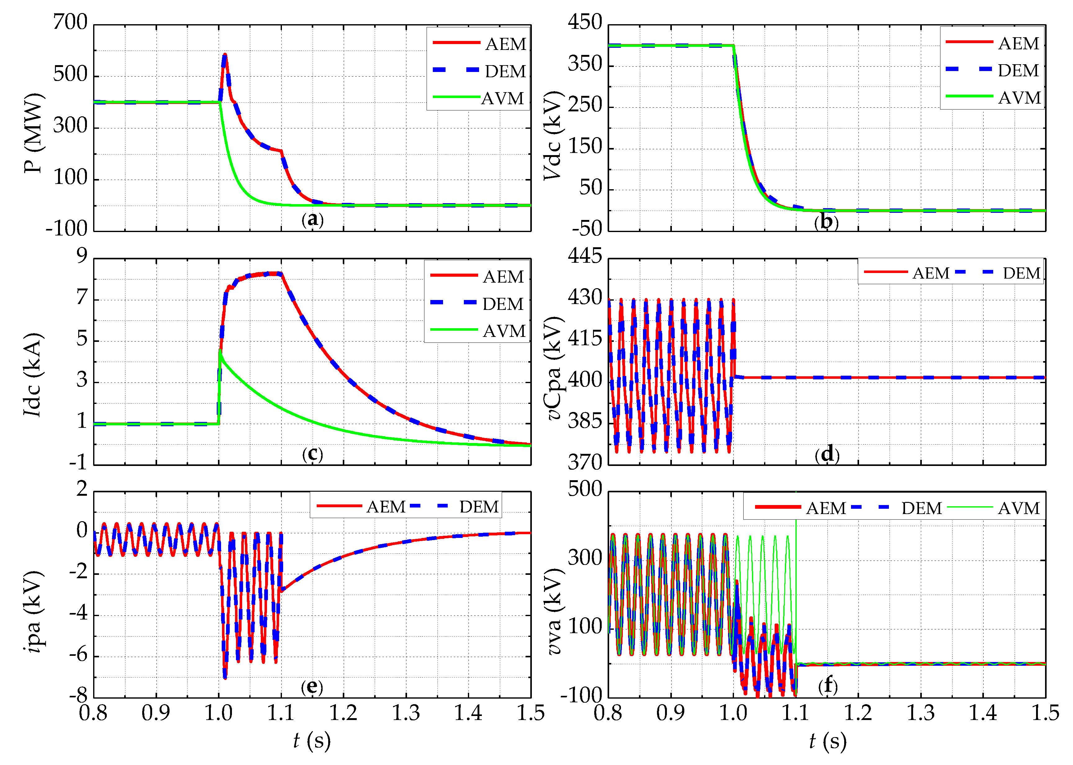
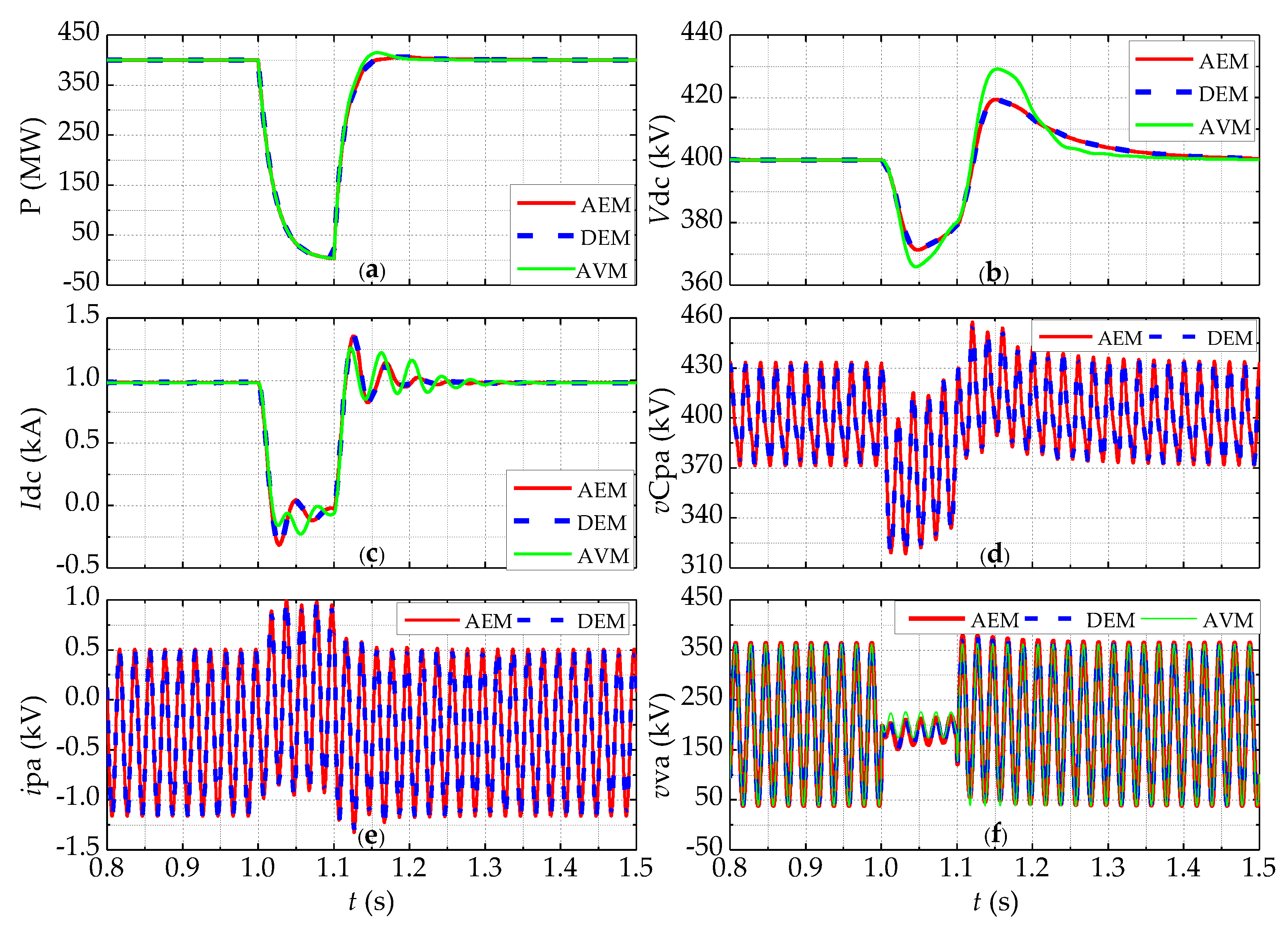
• The proposed AEM can more accurately reproduce the dynamics of the arm currents and the SM capacitor voltages compared to AVMs. The proposed AEM can reproduce the dynamic behaviors of the DEM under different scenarios very accurately, and is more computationally efficient with no loss of accuracy.
• The proposed AEM can accurately represent the dynamic responses in both de-blocked and blocked modes. Meanwhile, the ON-state and OFF-state resistances of the IGBT and its anti-parallel diodes in the SMs are accurately represented.
• The proposed AEM is verified against the DEM and AVM in a two-terminal MMC-HVDC system. The simulation results demonstrate the accuracy and computational efficiency of the proposed model in both de-blocked and blocked modes. Moreover, the simulation speed of the AEM is irrespective of the SM number.
• Except for the dynamics of individual SMs, the proposed AEM could be suitable for various simulation scenarios with no loss of accuracy, especially for large-scale MMC-HVDC grids.

This paper is organized as follows: Section 2 makes a brief introduction about the general structure, the control scheme, the DEM, and the AVM of the MMC. In Section 3, the arm equivalent model is derived based on average switching functions (ASFs). Based on the Thévenin’s theorem and nested fast and simultaneous solution, Section 4 describes the modelling process of the proposed AEM in detail. In Section 5, the accuracy and computational efficiency of the AEM is verified against the DEM and AVM, with several scenarios applied on the power systems computer aided design/ electromagnetic transient in DC system (PSCAD/EMTDC) program. Conclusions are drawn in Section 6.

2. General Structure, Control Scheme, and Previous Models of the MMC

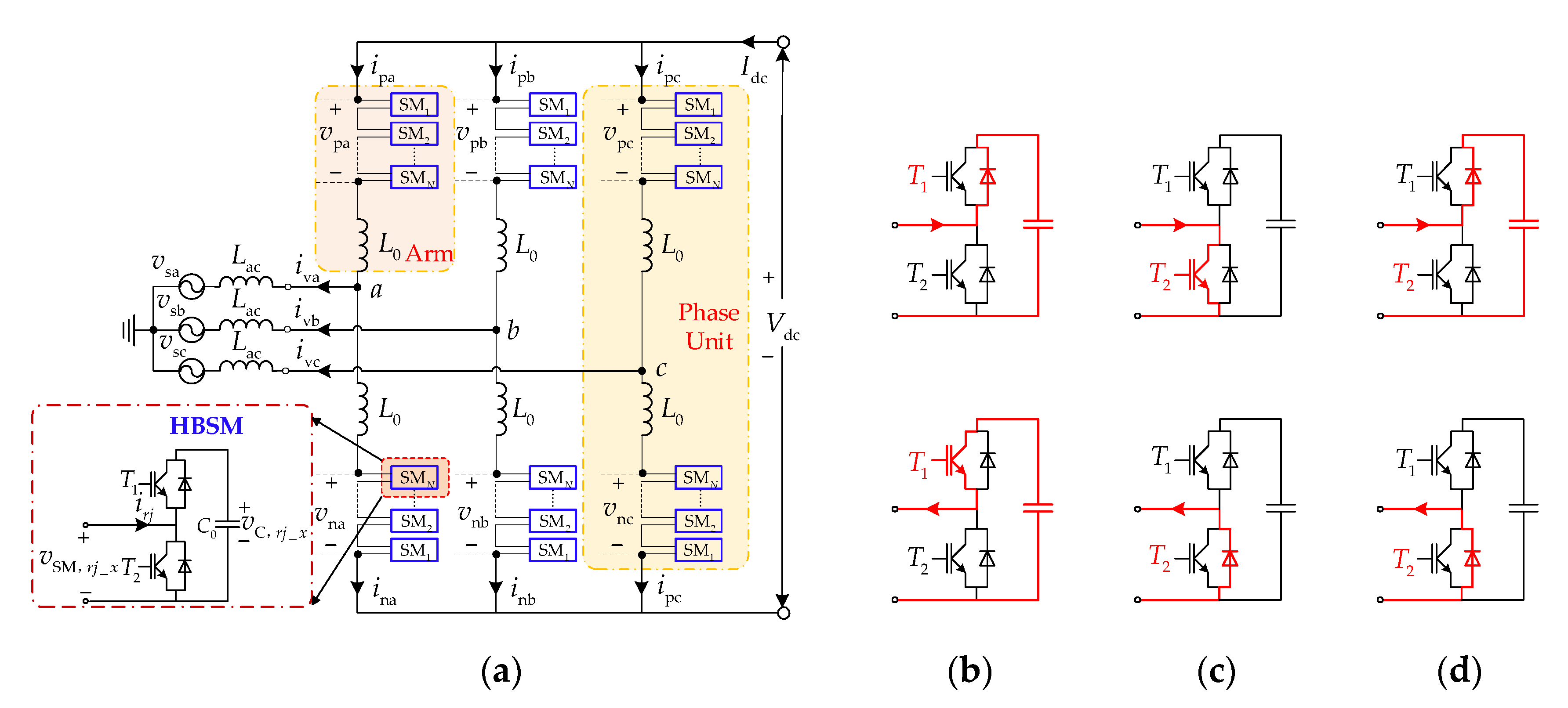
2.1. General Structure

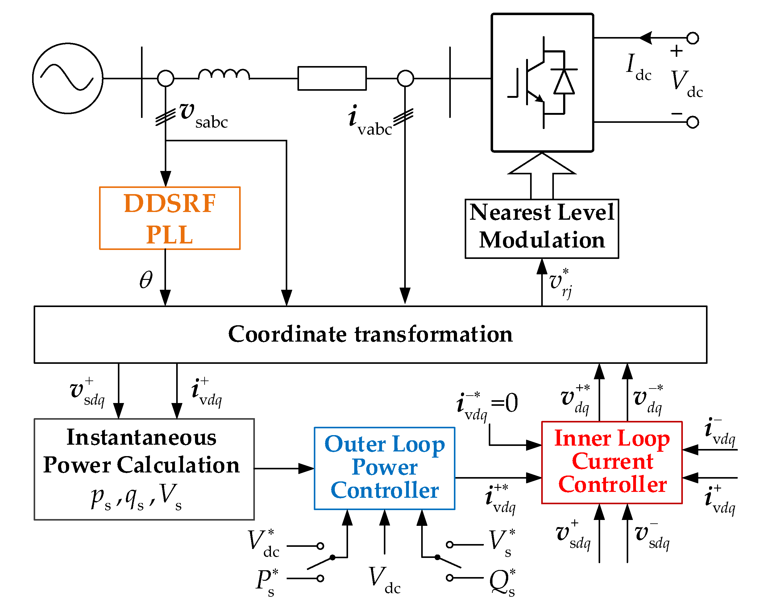
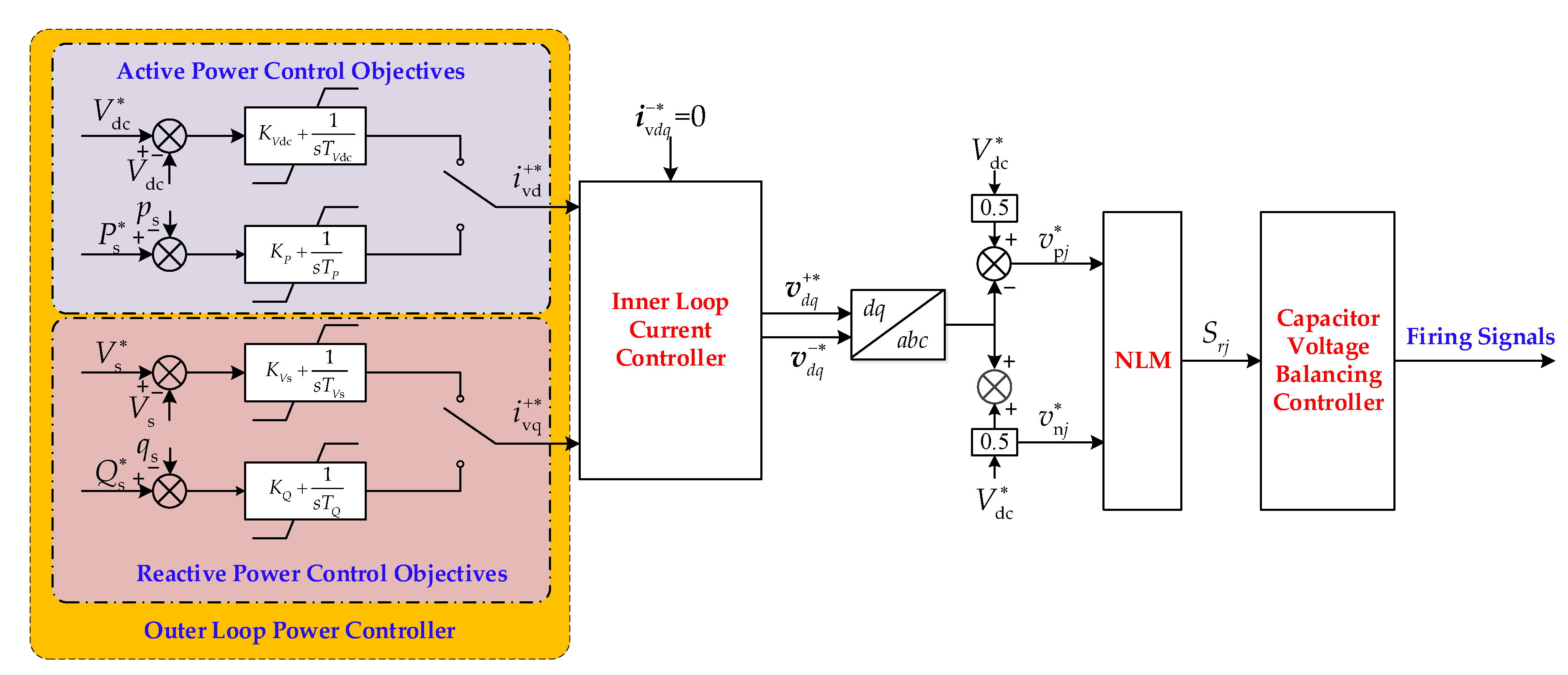
As illustrated in Figure 1a, the three-phase MMC consists of six arms, and each arm is composed of numerous half-bridge submodules (HBSMs) and an inductor (L₀) in series [20]. N is the number of HBSMs per arm. The arm voltage and the arm current are v_rj and i_rj, respectively. Here, the subscripts r (r = p, n) denote the upper and lower arms; j (j = a, b, c) denote one of the three phases. v_sj (v_sa, v_sb, and v_sc,) and i_vj (i_va, i_vb, and i_vc,) are the AC voltage and current in phase j at the AC side of the MMC, respectively; L_ac is the equivalent reactance of the AC system.

Each HBSM contains two IGBTs, two anti-parallel diodes and a capacitor (C₀). The firing signals of the two IGBTs are T₁ and T₂, respectively. v_{C, rj_x} is the voltage of the xth capacitor on the r arm in phase j; v_{SM, rj_x} is the output voltage of the xth SM on the r arm in phase j. As shown in Figure 1b–d, the current flow paths are highlighted in a red color, and the current flow paths rely on the current flow direction.

As shown in Figure 1b,c, under steady-state operation, each HBSM only has two states: (1) inserted mode (T₁ = 1, and T₂ = 0), v_{SM, rj_x} = v_{C, rj_x}, and the charging or discharging of the capacitor depends on the current flow direction; (2) bypassed mode (T₁ = 0, and T₂ = 1), v_{SM, rj_x} = 0, irrespective of the current flow direction. As depicted in Figure 1d, under abnormal operation (e.g., start-up, protective actions), the HBSM is blocked by switching off all IGBTs, and both T₁ and T₂ are set to zero. Two IGBTs are open circuit.

2.2. Control Scheme

As depicted in Figure 2, the vector current control based on the decoupled double synchronous reference frame phase-locked loop (DDSRF-PLL) is adopted for the MMC, which can completely eliminate the detection errors of conventional synchronous reference frame phase-locked loop (SRF-PLL) [21]. In Figure 2, v_sabc (v_sabc = [v_sa v_sb v_sc]^T) and i_vabc (i_vabc = [i_va i_vb i_vc]^T) are the three-phase voltage and current vectors at the AC side of the MMC, respectively; θ is the v_sabc phase angle detected by DDSRF-PLL; $v_{\mathrm{sdq}}^{+}\left(v_{\mathrm{sdq}}^{+}={\left[\begin{array}{cc}{v}_{\mathrm{sd}}& v_{\mathrm{vq}}\end{array}\right]}^{\mathrm{T}}\right)$ and $i_{\mathrm{vdq}}^{+}\left(i_{\mathrm{vdq}}^{+}={\left[\begin{array}{cc}{i}_{\mathrm{vd}}& i_{\mathrm{vq}}\end{array}\right]}^{\mathrm{T}}\right)$ are the dq axis positive-sequence voltage and current component vectors, respectively, and similarly for $v_{\mathrm{sdq}}^{-}$ $i_{\mathrm{vdq}}^{-}$, $i_{\mathrm{vdq}}^{+\ast }$, $i_{\mathrm{vdq}}^{-\ast }$, $v_{\mathrm{dq}}^{+\ast }$ and $v_{\mathrm{dq}}^{-\ast }$. Here, the superscripts + and − denote positive-sequence and negative-sequence components; the superscript $\ast$ denotes the command references of the variables. p_s and q_s are the instantaneous active and reactive power [22], and $P_{\mathrm{s}}^{\ast }$ and $Q_{\mathrm{s}}^{\ast }$ are the command references for the output active and reactive power of the MMC, respectively. $V_{\mathrm{dc}}^{\ast }$ is the DC voltage command reference, and $V_{\mathrm{s}}^{\ast }$ is the command reference for the amplitude of AC voltage v_sj.

The control scheme is decomposed to an outer-loop power controller and an inner-loop current controller [23]. According to the active- and reactive-power control objectives, the outer-loop power controller generates the dq axis positive-sequence current command references $i_{\mathrm{vd}}^{+\ast }$ and $i_{\mathrm{vq}}^{+\ast }$ for the inner loop current control, respectively. The inner-loop current controller regulates the dq axis positive-sequence current components ($i_{\mathrm{vdq}}^{+}$) at their references ($i_{\mathrm{vdq}}^{+\ast }$), and eliminate the negative-sequence current components ($i_{\mathrm{vdq}}^{-}$) with their references ($i_{\mathrm{vdq}}^{-\ast }$) set as zero, respectively [24]. Due to the conceptual and implementational simplicity, nearest level modulation (NLM) is adopted for a MMC with a high number of SMs [11].

2.3. Previous Models

2.3.1. Type A: Detailed Equivalent Models (DEMs)

DEMs reduce the size of the admittance matrix (Y) and the simulation burden of the MMC significantly, and the individual dynamics of every SM are still depicted [12]. As shown in Figure 3b, with the trapezoidal integration method, each SM capacitor is represented by an equivalent history voltage source in series with a resistance R_{C0, x} = ΔT/(2C₀), where ΔT denotes the simulation time-step. Then, based on Thévenin’s theorem, the xth SM equivalent circuit in Figure 3c is obtained:

$$v_{\mathrm{SM},x}\left(t\right)=R_{\mathrm{SMEQ},x}{i}_{\mathrm{SM},x}\left(t\right)+V_{\mathrm{SMEQ},x}\left(t-\Delta T\right)$$

(1)

where

$$R_{\mathrm{SMEQ},x}=\frac{R_{\mathrm{l},x}\left(R_{\mathrm{u},x}+R_{\mathrm{C}0,x}\right)}{R_{\mathrm{u},x}+R_{\mathrm{l},x}+R_{\mathrm{C}0,x}}$$

(2)

$$V_{\mathrm{SMEQ},x}\left(t-\Delta T\right)=\frac{R_{\mathrm{l},x}}{R_{\mathrm{u},x}+R_{\mathrm{l},x}+R_{\mathrm{C}0,x}}{V}_{\mathrm{C}0,x}\left(t-\Delta T\right)$$

(3)

where, v_{SM, x}(t) and i_{SM, x}(t) denotes the voltage and current of the xth SM at time t, respectively; V_{SMEQ, x}(t − ΔT) denotes the equivalent history output voltage of the xth SM at earlier time t − ΔT, and V_{C0, x}(t − ΔT) denotes the equivalent history capacitor voltage of the xth SM capacitor at earlier time t − ΔT; the values of resistor R_{u, x} (similarly, R_{l, x}) are either a low resistance R_on at ON-state or a large resistance R_off at OFF state, which depends on the switch state [25]. Then, for the arm in series with N SMs, the arm equivalent circuit can be constructed as in Figure 3d, where, the arm current i_Arm(t) = i_{SM, x}(t),

$$R_{\mathrm{Arm}}={\displaystyle \sum _{x=1}^N{R}_{\mathrm{SMEQ},x}}$$

(4)

$$V_{\mathrm{Arm}}\left(t-\Delta T\right)={\displaystyle \sum _{x=1}^N{V}_{\mathrm{SMEQ},x}\left(t-\Delta T\right)}$$

(5)

Here, V_{Arm, x}(t − ΔT) denotes the equivalent history arm voltage of xth SM at earlier time t − ΔT; v_Arm(t) is the arm voltage at time t.

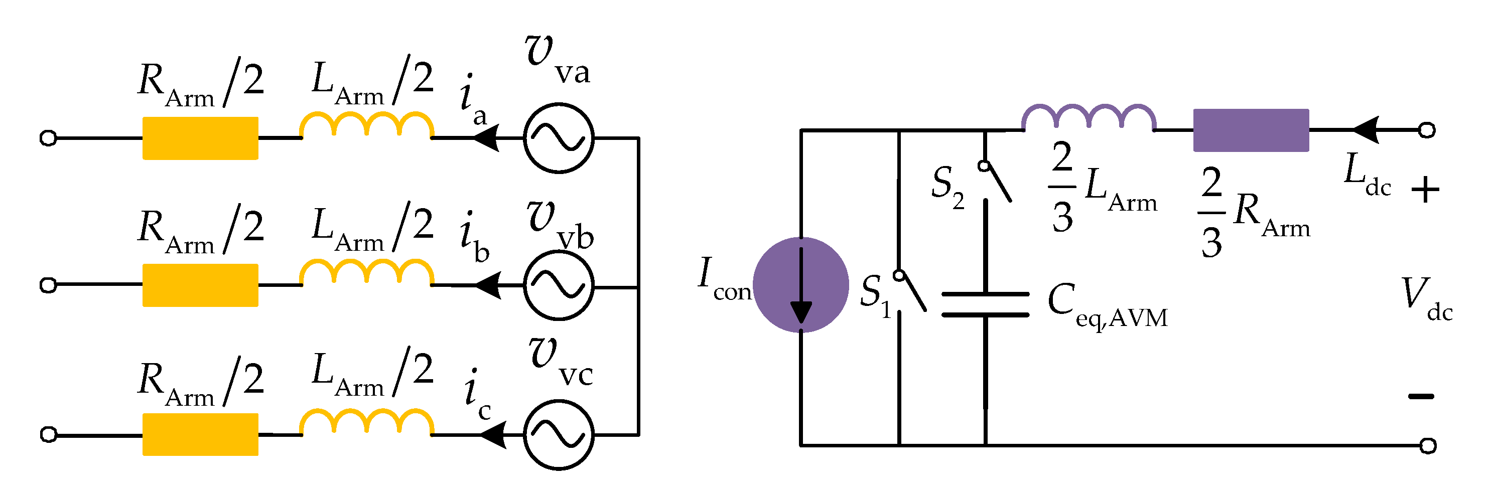
2.3.2. Type B: Average Value Models (AVMs)

The AVMs neglect the impact of SM capacitor ripple voltage by using a single equivalent capacitance, and further improve the simulation efficiency. The AVMs have less accurate simulations compared to the DEMs [15].

A brief overview of the AVM is expressed here, and a further description is given in [13]. As shown in Figure 4, the IGBTs are not explicitly represented and the behaviour of the MMC is modelled with the controlled voltage sources (v_vj) and controlled current source (I_con), where

$$v_{\mathrm{v}j}=v_{\mathrm{ref}, \mathrm{v}j}\frac{V_{\mathrm{dc}}}{2}$$

(6)

$$I_{\mathrm{con}}=\frac{1}{2}{\displaystyle \sum _j^{}{v}_{\mathrm{ref},\mathrm{v}j}{i}_j}$$

(7)

$$C_{\mathrm{eq},\mathrm{AVM}}=\frac{6C_0}{N}$$

(8)

where, v_ref,vj is the j phase voltage reference generated by the control system, which is a per-unit value; C_{eq, AVM} represents the DC-side equivalent capacitance; L_Arm (= L₀) and R_Arm (= NR_ON) denotes the arm equivalent inductance and resistance, respectively. Under de-blocked mode, the switch (S₁) is open, and S₂ is closed; under blocked mode, S₁ is closed to emulate the MMC blocking while switch S₂ is open. The dynamics under blocked mode are relatively inaccurate [15].

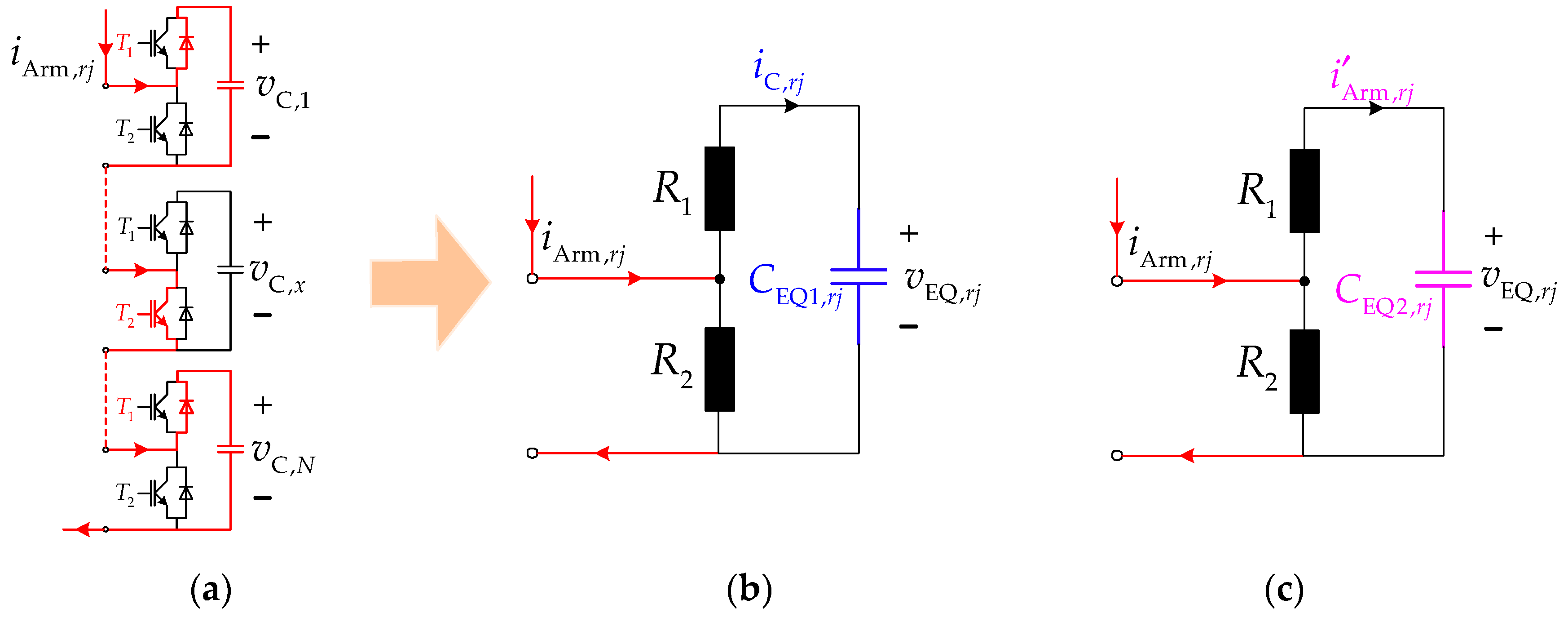
3. Equivalent Circuit of the MMC

In this Section, the arm equivalent circuits are only derived under de-blocked mode. The arm equivalence under blocked mode will be discussed in the next Section.

3.1. Average Capacitor Current of the SMs

The positive direction of the currents and voltages are shown in Figure 1a. As shown in Figure 1b, when the SM is under inserted mode, through the switching actions of power devices, the arm current is diverted into the capacitor branch of the SM. The current flowing through the capacitor is defined as the capacitor current. The capacitor current of the xth SM on the r arm in phase j i_{C, rj_x} is equal to the current flowing through the r arm in phase j i_{Arm, rj}. Namely, i_{C, rj_x} = i_{Arm, rj}. In contrast, i_{C, rj_x} is equal to zero for bypassed mode. Each SM is under only one mode at a specific moment. For the sake of convenience, i_{C, rj_x} is expressed as:

$$i_{\mathrm{C},rj\_x}=S_{rj\_x}{i}_{\mathrm{Arm},rj}$$

(9)

where, i_{Arm, rj} is the current flowing through the r arm in phase j; S_{rj_x} represents the switching function of the xth SM on the r arm in phase j, and is defined as:

$$S_{rj\_x}=\{\begin{array}{l}1,inserted \mathrm{mode} (T_1=1, T_2=0)\\ 0, bypassed \mathrm{mode} (T_1=0, T_2=1)\end{array}$$

(10)

Sum up the capacitor current of all N SMs on the specific arm, then:

$${\displaystyle \sum _{x=1}^N{i}_{\mathrm{C},rj\_x}}={\displaystyle \sum _{x=1}^N{S}_{rj\_x}{i}_{\mathrm{Arm},rj}}$$

(11)

so

$$\frac{1}{N}{\displaystyle \sum _{x=1}^N{i}_{\mathrm{C},rj\_x}}=i_{\mathrm{Arm},rj}\frac{1}{N}{\displaystyle \sum _{x=1}^N{S}_{rj\_x}}$$

(12)

As the number of SMs per arm N is very large, and the switching frequency is high enough, the inserted mode and bypassed mode for each SM are switching frequently. Therefore, the definition of the ASF is applied to represent the characteristic of SM frequent switching actions to simplify the analysis. For the sake of simplicity, the ASF is defined as S_rj to denote the average insertion ratio of the SMs on the r arm in phase j, and is expressed as [16,26]:

$$S_{rj}=\frac{1}{N}{\displaystyle \sum _{x=1}^N{S}_{rj\_x}}$$

(13)

In order to maintain the DC voltage V_dc stable, the sum of S_pj and S_nj in phase j is controlled as 1.

The average capacitor current of the SMs on the r arm in phase j i_{C, rj} is defined as:

$$i_{\mathrm{C},rj}=\frac{1}{N}{\displaystyle \sum _{x=1}^N{i}_{\mathrm{C},rj\_x}}$$

(14)

Note that, the sums of the currents in Equations (11) and (14) do not express the connection of SMs in parallel, but express the concept of SM average switching actions. From Equations (12) and (13), Equations (11) is rewritten as:

$$i_{\mathrm{C},rj}=S_{rj}{i}_{\mathrm{Arm},rj}$$

(15)

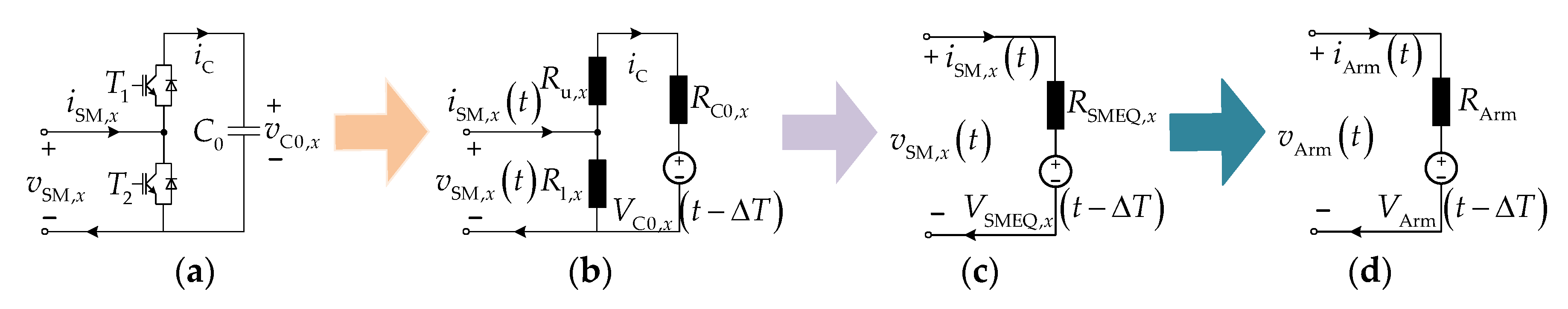
3.2. Equivalent Voltage of the Arm

Similarly to the average capacitor current, the output voltage of the xth SM on the r arm in phase j v_{sm, rj_x} is expressed as:

$$v_{\mathrm{sm},rj\_x}=S_{rj\_x}{v}_{\mathrm{C},rj\_x}$$

(16)

Sum up the voltage of all N SMs, then:

$${\displaystyle \sum _{x=1}^N{v}_{\mathrm{sm},rj\_x}}={\displaystyle \sum _{x=1}^N{S}_{rj\_x}{v}_{\mathrm{C},rj\_x}}$$

(17)

Suppose that all N SMs on an arm are identical, and all SM capacitor voltages are perfectly balanced [27,28], then the average capacitor voltage of each SM on the r arm in phase j v_{C, rj} is expressed as:

$$v_{\mathrm{C},rj}=v_{\mathrm{C},rj\_x}$$

(18)

Substitute Equations (12), (17) into Equation (16), and Equation (16) is rewritten as:

$${\displaystyle \sum _{x=1}^N{v}_{\mathrm{sm},rj\_x}}=S_{rj}\left(N{v}_{\mathrm{C},rj}\right)$$

(19)

From Equation (18), the equivalent output voltage on the r arm in phase j v_{EQ, rj} is defined as:

$$v_{\mathrm{EQ},rj}=S_{rj}\left(N{v}_{\mathrm{C},rj}\right)$$

(20)

3.3. Equivalent Voltage of the Arm

Based on the relationship between the voltage and current of the capacitor, the xth SM capacitor current i_{C, rj_x} can also be written as:

$$i_{\mathrm{C},rj\_x}=S_{rj\_x}{C}_0\frac{d{v}_{\mathrm{C},rj\_x}}{dt}$$

(21)

Sum up the capacitor current of all N SMs on the specific arm, then:

$${\displaystyle \sum _{x=1}^N{i}_{\mathrm{C},rj\_x}}=C_0{\displaystyle \sum _{x=1}^N{S}_{rj\_x}\frac{d{v}_{\mathrm{C},rj\_x}}{dt}}$$

(22)

Combine with Equation (18), then

$$\frac{1}{N}{\displaystyle \sum _{x=1}^N{i}_{\mathrm{C},rj\_x}}=C_0\frac{d{v}_{\mathrm{C},rj}}{dt}\left(\frac{1}{N}{\displaystyle \sum _{x=1}^N{S}_{rj\_x}}\right)$$

(23)

Substitute Equations (13), (14), (20) into Equation (23), and Equation (23) is rewritten as:

$$i_{\mathrm{C},rj}=\frac{C_0}{N}\frac{d{v}_{\mathrm{EQ},rj}}{dt}$$

(24)

According to Equation (23), the arm equivalent circuit based on the average capacitor current are shown in Figure 5b, which models the charging and discharging of the arm equivalent capacitor C_{EQ1, rj}, and can accurately represent the voltage ripples of the equivalent capacitor. The resistances R₁ and R₂ in Figure 5b,c are employed to take the losses of the power devices into account, whose values will be discussed later. In Figure 5b,c, the arm current mainly flows through the path marked in blue or purple color, and extremely weak current flows through R₂ due to the very large R₂.

C_{EQ1, rj} is expressed as:

$$C_{\mathrm{EQ}1,rj}=\frac{C_0}{N}$$

(25)

From (19), Equation (21) is re-derived as:

$$\frac{C_0}{N{S}_{rj}}\frac{d{v}_{\mathrm{EQ},rj}}{dt}=i_{\mathrm{Arm},rj}$$

(26)

According to Equation (26), the arm equivalent circuit based on arm current is replaced as in Figure 5c, which reflects the relationship between the arm equivalent output voltage and arm current, with an ASF-related equivalent capacitor C_{EQ2, rj}, and can exhibit the dynamics of the arm currents. In Figure 5c, the circuit ${i^{\prime }}_{\mathrm{Arm},rj}$ is very approximate to the arm current $i_{\mathrm{Arm},rj}$ due to the R₂ shunt effect. C_{EQ2, rj} is defined as:

$$C_{\mathrm{EQ}2,rj}=\frac{C_0}{N{S}_{rj}}$$

(27)

As shown in Figure 5b,c, compared with DSMs, the arm equivalence could drastically reduce the size of the nodes in the entire circuit and the computational intensity. The application for two arm equivalent circuits will be discussed in next Section.

3.4. Values of Resistances R₁ and R₂

An IGBT and its anti-parallel diode act as a bidirectional switch, and only one of them is conducted at a given instance. The switching actions can be treated as a two-state resistor: (1) ON state with a low resistance R_on; (2) OFF state with a large resistance R_off. Under a de-blocked state, for each arm, the sum of the SMs at inserted mode and bypassed mode is N at any instant. In other words, based on the current path as drawn in Figure 5a, the ON-state and OFF-state devices are always equal to N. Hence, based on the ASF, R₁, and R₂ are expressed as:

$$R_1=N{R}_{\mathrm{on}}$$

(28)

$$R_2=N{R}_{\mathrm{off}}$$

(29)

4. Modelling Process of the Proposed AEM

Most EMT simulation programs use Dommel’s algorithm [29]. Through the application of the trapezoidal integration, all dynamic elements are converted into a Norton equivalent current source in parallel with a conductance. Then, the admittance matrix equation of full circuit is formulated to solve the circuit, through the nodal analysis method (I =YU). Here, Y is the admittance matrix; U is the nodal voltage vector; I is the injection current vector that is renovated at each time-step, and is a function of the intrinsic sources and history terms arising from discrete companion components at earlier time-steps. By employing nested fast and simultaneous solution [19], the MMC circuit is decomposed into six arm subsystems, and a non-arm subsystem that excludes six arms. Each arm subsystem can be solved separately to a Thévenin equivalent circuit, which leads to a significant reduction in computation. Then, the Thévenin equivalent circuits of six arm subsystems are inserted in to the non-arm subsystem to solve the overall MMC-HVDC system. Through this approach, the arm with numerous SMs is reduced to a single 2-node element. Thus, the size of the admittance matrix (Y) of the overall circuit is drastically decreased, and the computational efficiency is significantly improved.

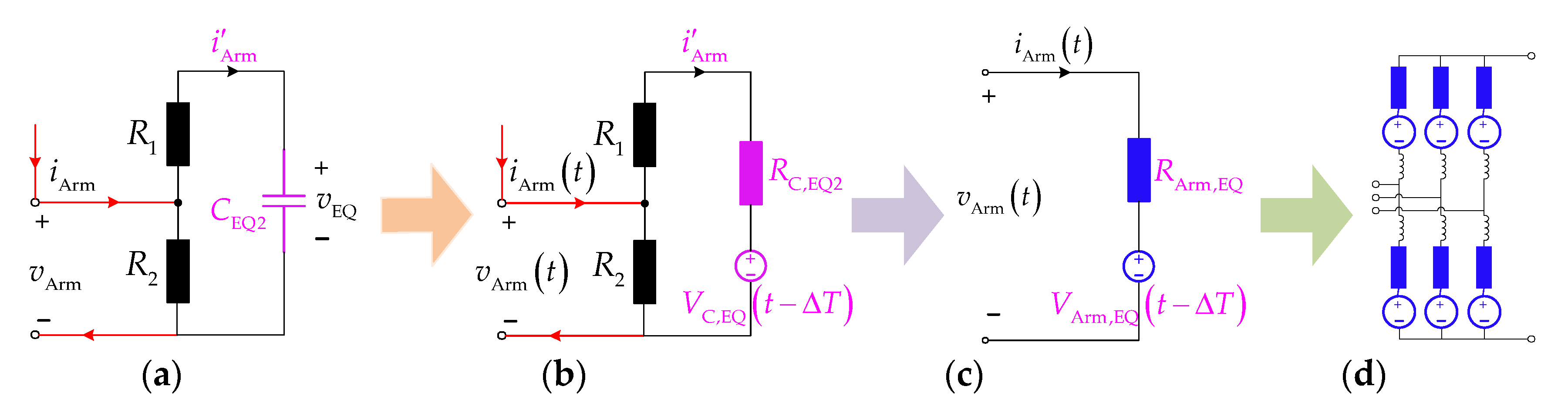
4.1. Thévenin Equivalent Circuit for the Arm on De-Blocked Model

Note that, the subscript rj is omitted later for simplicity. For the solution of the arm Thévenin equivalent circuit, the arm equivalent circuit based on arm current in Figure 5c is adopted.

Based on the trapezoidal integration method, the equivalent capacitor C_EQ2 is represented as an equivalent history voltage source V_{C, EQ}(t − ΔT) and a resistor R_{C, EQ2}, as in:

$$R_{\mathrm{C},\mathrm{EQ}2}=\frac{\Delta T}{2C_{\mathrm{EQ}2}}$$

(30)

The arm equivalent circuit inserted with C_EQ2 discrete companion model is shown in Figure 6b, where v_Arm(t) is the arm output voltage. Then, the Thévenin equivalent circuit of the arm is derived as in Figure 6c, whose parameters are as follows:

$$R_{\mathrm{Arm},\mathrm{EQ}}=\frac{R_2\left(R_1+R_{\mathrm{C},\mathrm{EQ}2}\right)}{R_1+R_2+R_{\mathrm{C},\mathrm{EQ}2}}$$

(31)

$$V_{\mathrm{Arm}, \mathrm{EQ}}\left(t-\Delta T\right)=\frac{R_2}{R_1+R_2+R_{\mathrm{C},\mathrm{EQ}2}}{V}_{\mathrm{C}, \mathrm{EQ}}\left(t-\Delta T\right)$$

(32)

4.2. Solution for the Equivalent Capacitor Voltage on De-Blocked Model

After the Thévenin equivalent circuit of the six arm subsystems at an earlier time-step is attained, as in Figure 6d, the entire circuit at the current time-step is finally solved by inserting the discrete companion models of the six arm subsystems into the non-arm subsystem. Then, the arm currents i_Arm(t) are obtained. According to the Figure 6b, the circuit ${i^{\prime }}_{\mathrm{Arm}}$ is calculated as:

$${i^{\prime }}_{\mathrm{Arm}}\left(t\right)=\frac{i_{\mathrm{Arm}}\left(t\right)R_2-V_{\mathrm{C},\mathrm{EQ}}\left(t-\Delta T\right)}{R_1+R_2+R_{\mathrm{C},\mathrm{EQ}2}}$$

(33)

From Equation (15), the average capacitor current i_C(t) at current time-step is expressed as:

$$i_{\mathrm{C}}\left(t\right)=S{i^{\prime }}_{\mathrm{Arm}}\left(t\right)$$

(34)

According to Figure 5b, the arm equivalent capacitor voltage v_EQ(t) at current time-step is calculated as:

$$v_{\mathrm{EQ}}\left(t\right)=R_{\mathrm{C},\mathrm{EQ}1}{i}_{\mathrm{C}}\left(t\right)+V_{\mathrm{C},\mathrm{EQ}}\left(t-\Delta T\right)$$

(35)

where,

$$R_{\mathrm{C},\mathrm{EQ}1}=\frac{\Delta T}{2C_{\mathrm{EQ}1}}$$

(36)

$$V_{\mathrm{C}, \mathrm{EQ}}\left(t-\Delta T\right)=R_{\mathrm{C},\mathrm{EQ}1}{i}_{\mathrm{C}}\left(t-\Delta T\right)+v_{\mathrm{EQ}}\left(t-\Delta T\right)$$

(37)

Here, i_C(t − ΔT) and v_EQ(t − ΔT) are the history of the average capacitor current and equivalent output voltage at an earlier time-step, respectively.

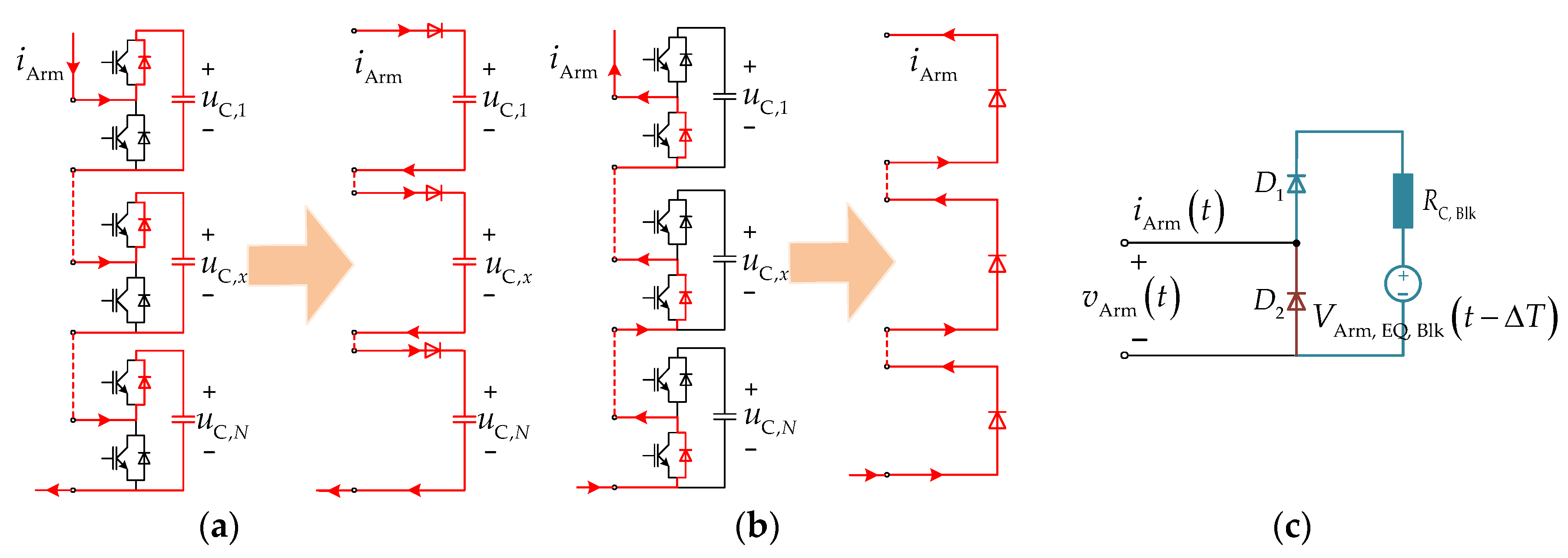
4.3. Thévenin Equivalent Circuit for the Arm on Blocked Model

Under blocked mode, all IGBTs on the arm are switched off, and the current path relies on the direction of the current. As shown in Figure 7a, when the current is positive, all capacitors on the arm are inserted in series into the arm, and the corresponding Thévenin equivalent circuit is depicted as the dark-green part in Figure 7c. Here,

$$R_{\mathrm{C}, \mathrm{Blk}}={\displaystyle \sum _{x=1}^N{R}_{\mathrm{C}0,x}}=\frac{N\Delta T}{2C_0}$$

(38)

$$V_{\mathrm{Arm}, \mathrm{EQ}, \mathrm{Blk}}\left(t-\Delta T\right)={\displaystyle \sum _{x=1}^N{V}_{\mathrm{C}0,\mathrm{EQ},x}\left(t-\Delta T\right)}=N{V}_{\mathrm{C}0,\mathrm{EQ}}\left(t-\Delta T\right)=R_{\mathrm{C}, \mathrm{Blk}}{i}_{\mathrm{Arm}}\left(t-\Delta T\right)+N{v}_{\mathrm{C}0}\left(t-\Delta T\right)$$

(39)

where, v_C0(t − ΔT) denotes the equivalent history voltage source of SM average capacitor voltage. Similarly to Equation (10), V_{C0, EQ}(t − ΔT) is equal to V_{C0, EQ, x}(t − ΔT). For negative current, alternatively, the current only flows through the diode D₂ as shown in Figure 7b,c.

As shown in Figure 7c, the blocked-state Thévenin circuit retains two static elements: the diodes D₁ and D₂ with negligible conductive resistances. The ON or OFF states of D₁ and D₂ directly depend on the EMT simulation programs, and do not need users to imitate their switching action. The solution for the equivalent capacitor voltage under blocked model is similar to the solution under de-blocked model, and is not discussed in this paper for the sake of conciseness.

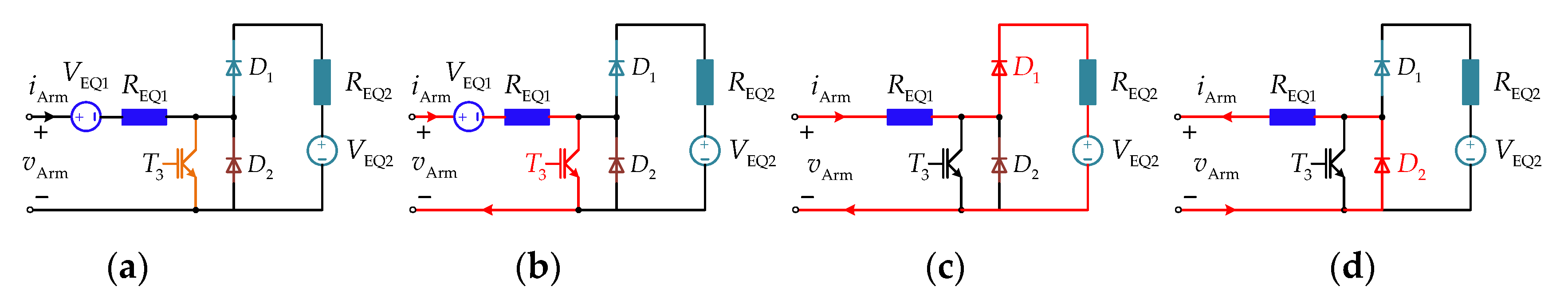
4.4. Thévenin Equivalent Circuit for Full States

The full-state Thévenin equivalent circuit is detailed in Figure 8a, where the IGBT T₃ is inserted in parallel with D₂ to switch the de-blocked or blocked modes. The T₃ is ON for de-blocked mode, or OFF for blocked mode. In Figure 8b–d, the paths that current flows through under different states are highlighted in red, respectively. The parameters of the equivalent circuit are listed in

Table 1. The parameters of the equivalent circuit.

State	Current Direction	T3	D1	D2	VEQ1	REQ1	VEQ2	REQ2
De-blocked	Positive	ON	OFF	OFF	Equation (32)	Equation (31)	0	0
	Negative	ON	OFF	ON	Equation (32)	Equation (31)	0	0
Blocked	Positive	OFF	ON	OFF	0	NRon	Equation (39)	Equation (38)
	Negative	OFF	OFF	ON	0	NRon	0	0

. Here, in blocked mode, R_EQ1 is assigned with NR_on to account for the conductive resistances of all diodes on the arm.

5. Simulation Studies

The DEM, the AVM, and the proposed AEM were implemented by using PSCAD/EMTDC. A two-terminal 200-level monopolar MMC-HVDC system was built to benchmark the accuracy and efficiency of the proposed AEM in comparison with the DEM and AVM. The MMC system and its parameters are illustrated in Figure 9 and

Table 2. The parameters of the MMC-HVDC.

MMC Converter
Items		Values	Items		Values
Rated capacity (MV·A)		400	Interface transformer	Rated capacity (MV·A)	480
AC system rated voltage RMS (kV)		230		Radio (kV/kV)	230/210
Rated DC voltage Vdc (kV)		400		Leakage reactance (p.u.)	0.15
Rated voltage of HBSM vC (kV)		2	Number of SMs per arm		200
HBSM capacitance C0 (mF)		6.67	Arm inductance L0 (mH)		33.77
Ron (Ω)		0.01	Roff (Ω)		1,000,000
Overhead DC Line
Items	Length (km)	+ ve Sequence R (Ω/km)		+ ve Sequence L (H/km)	+ ve Sequence C (F/km)
Value	100	9.735 × 10−3		8.489 × 10−4	1.367 × 10−8

, respectively. The MMC controllers depicted in Figure 10 were implemented in three models, and the SM capacitor voltage balancing control in [27] was adopted for the DEM. The MMC1 and MMC2 use P-Q and V_dc-Q controls, respectively. In Figure 10, K_Vdc, K_P, K_Vs, and K_Q are the proportional coefficients, and T_Vdc, T_P, T_Vs, and T_Q are the integral time constants of the proportional-integral (PI) regulator, respectively. Here, K_Vdc = 10, K_P = 0.64, K_Vs = 0.20, K_Q = 0.21, T_Vdc = 0.01 s, T_P = 0.0165 s, T_Vs = 0.0025 s, and T_Q = 0.029 s

The simulation time step was 20 μs. In the following simulation results, the SM capacitor voltage of the DEM was the sum of all individual SM capacitor voltages on the upper arm in phase a of MMC1, and the arm current was observed on the upper arm in phase a of MMC1. Since the AVM does not have the capacity to represent the arm dynamics, the arm current and SM capacitor voltages of the AEM and DEM, only, were compared.

5.1. Steady State

At t = 1.0 s, The P reference of MMC1 stepped from 200 MW to 400 MW. The MMC1 transients due to the change of the P reference are shown in Figure 11. As the active power was regulated to 400 MW at t = 1.0 s, the DC current rose from 0.5 kA to 1 kA, which led to higher SM capacitor voltage ripples, as shown in Figure 11d. The current rise rate of the AVM was slightly slower than the other two models.

From Figure 11, the dynamics of the proposed AEM very accurately reproduced the responses of the DEM. Especially in Figure 11d, the ripple of the equivalent capacitor voltage for the AEM is essentially identical to the sum of all individual SM capacitor voltages for the DEM, which proves the accuracy of the proposed AEM. Compared to the AEM and DEM, only the AC voltage in phase a at valve-side was the same as the other models. Nevertheless, the AVM shows low accuracy on the DC side, where only the variation trends of DC voltage and DC current were similar.

5.2. DC-Side Pole-to-Ground Fault

At t = 1.0 s, a DC-side pole-to-ground permanent fault was applied in the middle of the overhead DC line, as shown in Figure 9. For the AEM and DEM, both MMC1 and MMC2 were blocked at 2 ms after the DC fault occurred. For the AVM, S₁ was closed, and S₂ was open at 1.002 s. The AC breakers were opened at t = 1.1 s. The responses of the three models are shown in Figure 12.

After the fault occurred, the DC voltage dropped sharply, as in Figure 12b, and the MMCs immediately contributed the fault current to the DC fault location. As shown in Figure 12c, the DC currents rose sharply as the SM capacitor discharge current became the dominant component, resulting in the active power of MM1 increasing, and SM capacitor voltages reducing successively. After blocking the MMCs, the SM capacitor was no longer discharged, thus staying constant, as shown in Figure 12d. Therefore, the fault current from the AC system became the dominant component. After the ACCB is tripped, the residual DC fault currents will gradually decay through the R-L damping loop [30,31]. Due to the large decay time constant in the damping loop, it takes a long time (about 0.4 s) for the fault DC current to decay to zero [30].

It was observed that the trends of the DC fault currents for three models were similar before blocking the MMCs, since the DC-side equivalent fault circuits were similar [30]. After blocking the MMCs, the proposed AEM very accurately reproduced the transient responses of the DEM. Compared to the AEM and DEM, only the DC voltage was similar to the other models. Since the AC side and DC side of AVM are decoupled, the capacitor C_{eq, AVM} is disconnected after blocking the MMCs, leading to the incorrect dynamics, especially for the active power and DC current. This simulation scenario directly reflected that the AVMs have difficulty achieving accurate results under blocked mode.

Therefore, the proposed AEM can accurately reproduce the dynamic responses in both de-blocked and blocked modes.

5.3. AC-Side Three-Phase-to-Ground Fault

A three-phase-to-ground fault is applied to the MMC1 primary side at t = 1.0 s, and is cleared after 0.1 s (t = 1.1 s). Figure 13 illustrates the simulation waveforms of three models. After the AC fault occurred, the AC voltage at the MMC1 primary side dropped to zero, thus leading to the active power and DC current reducing to zero. Due to the insufficient active power at the DC side, the DC voltage and SM capacitor voltage decreased. After clearing the AC fault, and with the active power gradually recovered, the DC voltage gradually increased to the rated value. As in Figure 13b, the variation amplitude of DC voltage for the AVMs was larger than the other two models. The current waveform of the AVMs was significantly different from the other models during the fault.

As in Figure 13, the proposed AEM accurately matches the transient responses of the DEM, while the AVM cannot properly replicate the transient responses of the DEM. Comprehensively considering the Section 5.1, Section 5.2 and Section 5.3, the proposed AEM is suitable for various scenarios with no loss of accuracy; the AVM is more suitable for studying the AC side dynamics of MMC, while the DC side dynamics are somewhat inaccurate.

5.4. Computational Performance

A 1.0-s simulation study for the test system in Figure 9 was executed on a PC with 3.6 GHz Intel core i7-7700 HQ with 32 GB RAM under Microsoft Windows 10 operating system. Different numbers of SMs per arm were employed in the simulation studies to represent different complexities of test systems. The simulation execution times for the three models are summarized in

Table 3. Execution times for the three models.

Number of SMs per Arm	CPU Time (s)
	AEM	DEM	AVM
150	8.1	18.4	5.6
200	8.1	21.7	5.5
250	8.2	25.1	5.5
300	8.2	28.5	5.6
350	8.1	31.8	5.5
400	8.2	35.5	5.6

.

From Table 3, the DEM required longer simulation execution times, as the number of SMs per arm increased, since all SMs were considered separately and all individual capacitor voltage ripples were recorded. However, the proposed AEM requires the same execution time regardless of the number of the SMs per arm, as all SMs do not have to be considered separately, due to the arm equivalence. The proposed AEM was about only 45% slower than the AVM, and was more than three times faster than the DEM in terms of simulation efficiency. Hence, Table 3 demonstrates that the proposed model can be efficiently suitable for large-scale MMC-HVDC grids. In conclusion, the proposed AEM not only has an accuracy consistent with DEMs, but also has a satisfactory simulation efficiency compared to the AVMs.

6. Conclusions

This paper proposed an enhanced computationally efficient model for MMC based on arm equivalence. The proposed AEM could accurately reproduce the dynamic responses in both de-blocked and blocked modes, and has significant computational efficiency, especially for the large-scale MMC-HVDC grids. Based on a two-terminal monopolar MMC-HVDC system built on the PSCAD/EMTDC program, the accuracy and efficiency of the proposed AEM was verified against the DEM and AVM, with several simulation scenarios, where both de-blocked and blocked modes were considered. The simulation results demonstrated that:

• The proposed model can accurately represent the dynamics of the arm currents and SM capacitor voltages compared to AVM. In terms of simulation efficiency, the proposed AEM is only about 45% slower than the AVM, and is more than three times faster than the DEM.
• Compared to the DEM, the proposed AEM very accurately reproduces the dynamic behaviors of the DEM under different scenarios, and affords a substantial acceleration in simulation speed, with no loss of accuracy. Except for the dynamics of individual SMs, the proposed AEM could be suitable for various simulation scenarios with no loss of accuracy.
• The proposed AEM consumes the same amount of execution time regardless of the number of the SMs per arm, thus it can be efficiently adopted for large-scale MMC-HVDC grids with high computational speed.
• Although the simulation efficiency of AVMs is satisfactory, they lose accuracy compared to DEMs, especially for the blocked mode. Thus, the AVMs are suitable for system-level studies, which mainly focus on the steady-state dynamics and responses of AC fault.

Thereby, the proposed AEM has a higher computational efficient with no loss of accuracy, which is desirable for studies of large-scale MMC-HVDC grids with large numbers of SMs.

References

1. Qin, B.; Liu, W.; Zhang, R.; Liu, J.; Li, H. Review on short-circuit current analysis and suppression techniques for MMC-HVDC transmission systems. Appl. Sci. 2020, 10, 6769. [Google Scholar] [CrossRef]
2. Diaz, M.; Cárdenas Dobson, R.; Ibaceta, E.; Mora, A.; Urrutia, M.; Espinoza, M.; Rojas, F.; Wheeler, P. An overview of applications of the modular multilevel matrix converter. Energies 2020, 13, 5546. [Google Scholar] [CrossRef]
3. Wang, Z.; Lin, H.; Ma, Y. A control strategy of modular multilevel converter with integrated battery energy storage system based on battery side capacitor voltage control. Energies 2019, 12, 2151. [Google Scholar] [CrossRef] [Green Version]
4. Liu, G.; Xu, F.; Xu, Z.; Zhang, Z.; Tang, G. Assembly HVDC breaker for HVDC grids with modular multilevel converters. IEEE Trans. Power Electron. 2017, 32, 931–941. [Google Scholar] [CrossRef]
5. Zhang, Z.; Xu, Z.; Xu, T. Calculating current and temperature fields of HVDC grounding electrodes. J. Mod. Power Syst. Clean Energy 2016, 4, 300–307. [Google Scholar] [CrossRef]
6. Qin, B.; Li, H.; Zhou, X.; Li, J.; Liu, W. Low-voltage ride-through techniques in DFIG-based wind Turbines: A review. Appl. Sci. 2020, 10, 2154. [Google Scholar] [CrossRef] [Green Version]
7. Debnath, S.; Qin, J.; Bahrani, B.; Saeedifard, M.; Barbosa, P. Operation, control, and applications of the modular multilevel converter: A review. IEEE Trans. Power Electron. 2015, 30, 37–53. [Google Scholar] [CrossRef]
8. Cigre Working Group B4-57. Guide for the Development of Models for HVDC Converters in a HVDC Grid: TB-604; Cigre Working Group B4-57: Paris, France, 2014. [Google Scholar]
9. Diaz, M.; Cardenas, R.; Ibaceta, E.; Mora, A.; Urrutia, M.; Espinoza, M.; Rojas, F.; Wheeler, P. An overview of modelling techniques and control strategies for modular multilevel matrix converters. Energies 2020, 13, 4678. [Google Scholar] [CrossRef]
10. Peralta, J.; Saad, H.; Dennetière, S.; Mahseredjian, J.; Nguefeu, S. Detailed and averaged models for a 401-level MMC-HVDC system. IEEE Trans. Power Deliv. 2012, 27, 1501–1508. [Google Scholar] [CrossRef]
11. Tu, Q.; Xu, Z. Impact of sampling frequency on harmonic distortion for modular multilevel converter. IEEE Trans. Power Deliv. 2011, 26, 298–306. [Google Scholar] [CrossRef]
12. Gnanarathna, U.N.; Gole, A.M.; Jayasinghe, R.P. Efficient modeling of modular multilevel HVDC converters (MMC) on electromagnetic transient simulation programs. IEEE Trans. Power Deliv. 2011, 26, 316–324. [Google Scholar] [CrossRef] [Green Version]
13. Ajaei, F.B.; Iravani, R. Enhanced equivalent model of the modular multilevel converter. IEEE Trans. Power Deliv. 2015, 30, 666–673. [Google Scholar] [CrossRef]
14. Xu, J.; Gole, A.M.; Zhao, C. The use of averaged-value model of modular multilevel converter in DC grid. IEEE Trans. Power Deliv. 2015, 30, 519–528. [Google Scholar] [CrossRef]
15. Beddard, A.; Sheridan, C.E.; Barnes, M.; Green, T.C. Improved accuracy average value models of modular multilevel converters. IEEE Trans. Power Deliv. 2016, 31, 2260–2269. [Google Scholar] [CrossRef]
16. Song, Q.; Liu, W.; Li, X.; Rao, H.; Xu, S.; Li, L. A steady-state analysis method for a modular multilevel converter. IEEE Trans. Power Electron. 2013, 28, 3702–3713. [Google Scholar] [CrossRef]
17. Liu, M.; Li, Z.; Yang, X. A universal mathematical model of modular multilevel converter with half-bridge. Energies 2020, 13, 4464. [Google Scholar] [CrossRef]
18. Corazza, G.; Someda, C.; Longo, G. Generalized thevenin’s theorem for linear N-port networks. IEEE Trans. Circuit Theory 1969, 16, 564–566. [Google Scholar] [CrossRef]
19. Strunz, K.; Carlson, E. Nested fast and simultaneous solution for time-domain simulation of integrative power-electric and electronic systems. IEEE Trans. Power Deliv. 2007, 22, 277–287. [Google Scholar] [CrossRef]
20. Tu, Q.; Xu, Z.; Xu, L. Reduced switching-frequency modulation and circulating current suppression for modular multilevel converters. IEEE Trans. Power Deliv. 2011, 26, 2009–2017. [Google Scholar]
21. Rodriguez, P.; Pou, J.; Bergas, J.; Candela, J.I.; Burgos, R.P.; Boroyevich, D. Decoupled double synchronous reference frame PLL for power converters control. IEEE Trans. Power Electron. 2007, 22, 584–592. [Google Scholar] [CrossRef]
22. Akagi, H.; Watanbe, E.H.; Aredes, M. Instantaneous Power Theory and Applications to Power Conditioning; IEEE Press/Wiley-Interscience: Piscataway, NJ, USA, 2007. [Google Scholar]
23. Xu, L.; Andersen, B.; Cartwright, P. VSC transmission operating under unbalanced AC conditions–Analysis and control design. IEEE Trans. Power Deliv. 2005, 20, 427–434. [Google Scholar] [CrossRef]
24. Guan, M.; Xu, Z. Modeling and control of a modular multilevel converter-based HVDC system under unbalanced grid conditions. IEEE Trans. Power Electron. 2012, 27, 4858–4867. [Google Scholar] [CrossRef]
25. Manitoba Hydro International Ltd. PSCAD User’s Guide v4.6. 2018. Available online: https://www.pscad.com/knowledge-base/article/160 (accessed on 10 October 2020).
26. Xiao, H.; Xu, Z.; Tang, G.; Xue, Y. Complete mathematical model derivation for modular multilevel converter based on successive approximation approach. IET Power Electron. 2015, 8, 2396–2410. [Google Scholar] [CrossRef]
27. Liu, G.; Xu, Z.; Xue, Y.; Tang, G. Optimized control strategy based on dynamic redundancy for the modular multilevel converter. IEEE Trans. Power Electron. 2015, 30, 339–348. [Google Scholar] [CrossRef]
28. Nguyen, M.H.; Kwak, S. Improved indirect model predictive control for enhancing dynamic performance of modular multilevel converter. Electronics 2020, 9, 1405. [Google Scholar] [CrossRef]
29. Dommel, H.W. Digital computation of electromagnetic transients in single and multi-phase networks. IEEE Trans. Power App. Syst. 1969, PAS-88, 388–399. [Google Scholar] [CrossRef]
30. Xu, Z.; Xiao, H.; Xiao, L.; Zhang, Z. DC fault analysis and clearance solutions of MMC-HVDC systems. Energies 2018, 11, 941. [Google Scholar] [CrossRef] [Green Version]
31. Wang, S.; Alsokhiry, F.S.; Adam, G.P. Impact of submodule faults on the performance of modular multilevel converters. Energies 2020, 13, 4089. [Google Scholar] [CrossRef]
Figure 1. The general structure of the modular multilevel converters (MMC), and three modes of half-bridge submodules (HBSM): (a) The general structure of the MMC; (b) Inserted mode; (c) Bypassed mode; (d) Blocked mode.
Applsci 10 08421 g001
Figure 2. Control scheme of the MMC.
Applsci 10 08421 g002
Figure 3. The detailed equivalent models (DEM) topology: (a) The HBSM; (b) The submodule (SM) equivalent circuit, with companion model; (c) The SM Thévenin equivalent circuit; (d) The arm Thévenin equivalent circuit.
Applsci 10 08421 g003
Figure 4. The average value model (AVM) topology.
Applsci 10 08421 g004
Figure 5. The arm equivalence: (a) The general structure of the arm; (b) The arm equivalent circuit based on average capacitor current; (c) The arm equivalent circuit based on arm current.
Applsci 10 08421 g005
Figure 6. The Thévenin equivalent process: (a) The arm equivalent circuit based on arm current; (b) The arm equivalent circuit with RC, EQ2 discrete companion model; (c) Thévenin equivalent circuit of the arm; (d) The equivalent circuit of the MMC.
Applsci 10 08421 g006
Figure 7. The Thévenin equivalent process in the blocked state: (a) The positive direction of the current; (b) The negative direction of the current; (c) Thévenin equivalent circuit of the arm in the blocked state.
Applsci 10 08421 g007
Figure 8. The Thévenin equivalent circuit for full states: (a) Thévenin equivalent circuit; (b) Steady state; (c) Positive current at blocked state; (d) Negative current at blocked state.
Applsci 10 08421 g008
Figure 9. The two-terminal monopolar MMC-HVDC system.
Applsci 10 08421 g009
Figure 10. The control schematic of the MMC-HVDC system.
Applsci 10 08421 g010
Figure 11. Steady state: (a) MMC1 active power; (b) DC voltage; (c) DC current; (d) SMs capacitor voltage; (e) Current in upper arm in phase a; (f) AC voltage in phase a at valve-side.
Applsci 10 08421 g011
Figure 12. DC fault. (a) MMC1 active power; (b) DC voltage; (c) DC current; (d) SMs capacitor voltage; (e) Current on the upper arm in phase a; (f) AC voltage in phase a at valve-side.
Applsci 10 08421 g012
Figure 13. AC fault. (a) MMC1 active power; (b) DC voltage; (c) DC current; (d) SMs capacitor voltage; (e) Current in the upper arm in phase a; (f) AC voltage in phase a at valve-side.
Applsci 10 08421 g013