Model-Based Design and Simulation of Paraxial Ray Optics Systems

Abstract

A model-based design allows representing complex, multi-domain systems as interconnected functional blocks, yielding graphical, intuitive information about the overall project, besides simplifying simulation. This work proposes using the modular approach as an optical engineering design and educational tool for developing paraxial ray optics setups, providing further integration with mechatronics subsystems and control loops. An expanded version of the ABCD transfer matrix modeling is implemented in MATLAB Simulink environment to simultaneously perform ray tracing and dynamic simulations. The methodology is validated for different problems, including paraxial cloaking, transmission through a multimode optical fiber, a Fabry–Perot interferometer, and an optical pickup with automatic focus, yielding reliable results with prospective applications in optical engineering design and for creating virtual labs devoted to multiphysics and mechatronics engineering courses.

1. Introduction

A model-based design allows describing complex, multi-domain systems as interconnected modules that represent components of the overall project. In a mechatronics concept, mechanical, electrical, and magnetic subsystems communicate through input/output signals from sensors, actuators, control loops, and artificial intelligence. This approach simplifies the model identification and evaluation, and can be used to validate the system response to several inputs [1]. Simulation is also beneficial to the e-learning experience: virtual labs provide a feasible environment for testing analytical projects, besides reducing the time and infrastructure costs demanded by physical experiments [2,3].

Regarding the development of optical systems, typical examples of multi-domain implementations comprise beam monochromators [4], auto-focusing systems for imaging and disk readers [5], 3D scanners [6], and optoelectronic transducers [7]. Apart from wave, electromagnetic, and quantum optics approaches, geometrical optics is a straightforward and simpler way for tracing the light path in terms of successive transmission, reflection, and refraction, with notable applications in imaging systems [8], illumination [9], optometry [10], and computer graphics [11].

Although a variety of commercial and open-source software for ray tracing is currently available [12,13,14], integrating multiple physical domains into a unique simulation environment is still a challenge, especially regarding implementations in optomechatronics, wherein the optical system must be updated in response to the stimuli from the electromechanical module, while the information provided by the optical setup is applied as a feedback to the control loop. Moreover, the computer program should be accessible and easy-to-use, present a graphical programming interface that resembles the physical placement of components, and communicate with third-party applications.

In this sense, using MATLAB (Mathworks) or LabVIEW (National Instruments) is a convenient way to adapt custom-made ray optics functions to the available multi-domain models, with perspectives for real-time and hardware-in-loop implementations. For instance, script-based MATLAB libraries were proposed to evaluate paraxial optical systems [15,16], whereas in [17], the Simulink environment was applied to compute the mechanical response. At the same time, light trajectory is displayed using CODE V (Synopsys). Concurrent calculations in the optical, electrical, and mechanical domains were also carried out by Simulink for designing micro-scale devices [18] and telescopes [8], the latter communicates with external ray tracing software. Furthermore, control and tracing were conceived with LabVIEW to operate an instrumented testbed for aerospace applications [19]. Alternatively, one may use the Delano diagrams to evaluate power density and depict ray tracing in a compact notation that contains the comprehensive information provided by Gaussian optics without showing the explicit placement of optical components [20,21]. Despite the available works, a consolidated modeling and visualization environment for optical and multi-physical design is still required to fulfill the optical engineering design and educational purposes.

This paper proposes using MATLAB Simulink to develop model-based 2D paraxial optical and optomechatronics systems in unique software. Ray tracing is performed using the optics transfer matrices, wherein the position and orientation of light rays vary over time according to the simulation results for dynamically updating the tracing profile. Moreover, programming is facilitated by graphical language since the optical components are presented as functional blocks, wherein the interface with mechanical and electrical domains is settled with appropriate transducers. Using such a unified simulation environment is simpler than integrating different visualization and data processing software; besides, it is suitable for developing closed-loop projects that involve dynamic interaction between the electromechanical and optical parts. The main objective is to provide the bases for establishing virtual labs in physics and engineering design rather than conceiving intricate projects as in the aforementioned works; nevertheless, it can be used by researchers to develop and validate basic optical systems.

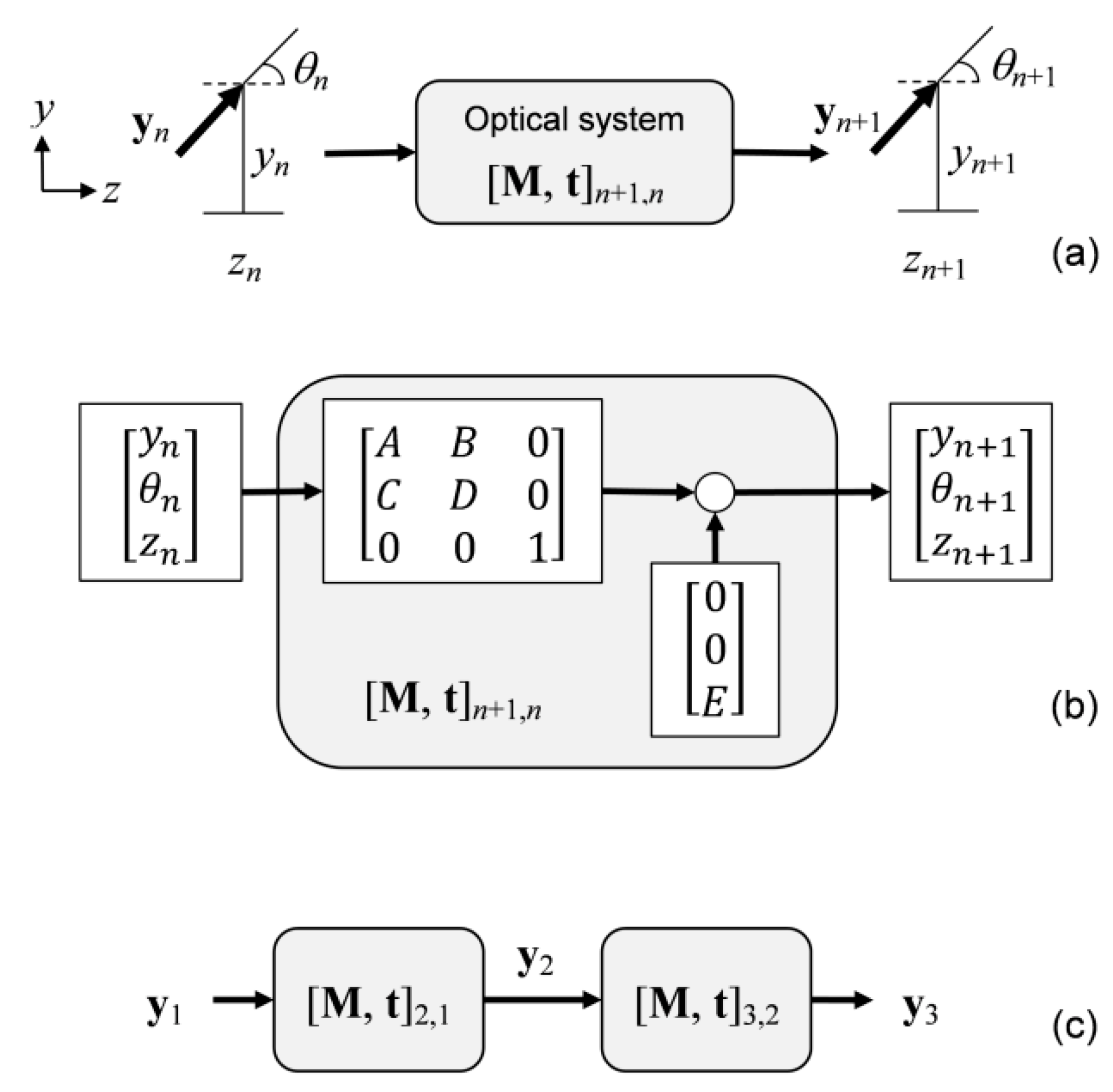
2. Ray Transfer Matrix

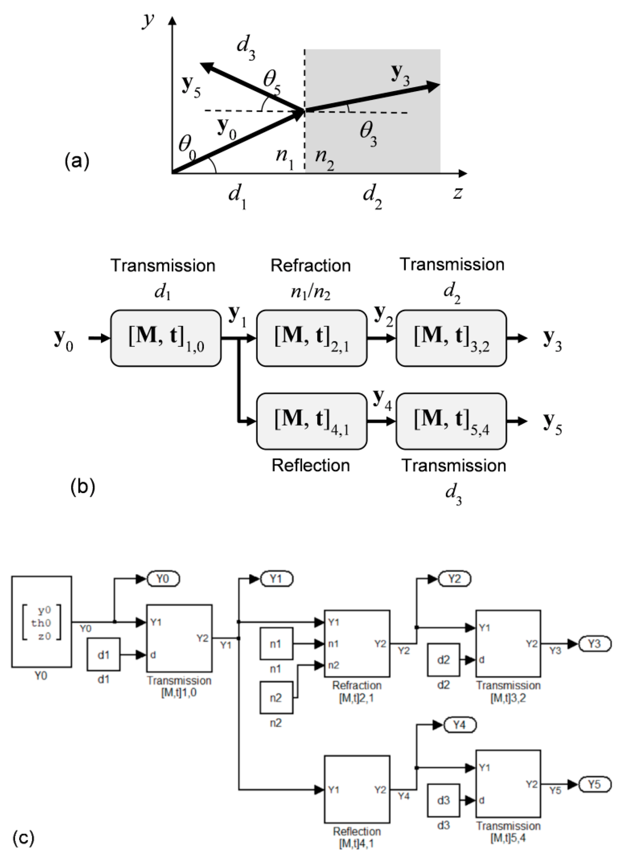
According to the theory of ray optics, light propagating in yz-plane along z-direction is described by its height y and orientation θ. For small angles (sin θ ≈ θ), rays can be treated by the paraxial approximation so that the correlation between output and input light due to an optical element is given by a linear system. The response of complex optical systems can be obtained by concatenating 2 × 2 ABCD matrices of each basic component like continuous media, mirrors, and lenses.

Instead of using the [y θ]^T convention from matrix optics, a 3 × 1 light array structure y = [y θ z]^T is used to include the position z for tracing purposes. The input ray y_n subjected to an optical component described by a 3 × 3 transfer matrix M_n+1,n and a 3 × 1 translation vector t_n+1,n yields the output y_n+1,

$$y_{n+1}=\left[\begin{array}{c}{y}_{n+1}\\ {\theta }_{n+1}\\ z_{n+1}\end{array}\right]=M_{n+1,n}{y}_n+t_{n+1,n}=\left[\begin{array}{ccc}A& B& 0\\ C& D& 0\\ 0& 0& 1\end{array}\right]\left[\begin{array}{c}{y}_n\\ {\theta }_n\\ z_n\end{array}\right]+\left[\begin{array}{c}0\\ 0\\ E\end{array}\right],$$

(1)

A, B, C, and D are the elements of the standard ray transfer matrix, and E updates the output ray position z_n+1, as shown in Figure 1. The optical component [M,t]_n+1,n represents the transformation from the state n to a subsequent state n+1. Although concatenating components is not mathematically straightforward as in conventional ABCD matrices, the modular design approach allows building and connecting subsystems similarly to block diagrams. For example, in Figure 1c, y₃ is obtained from y₁ by calculating y₃ = [M,t]_3,2[M,t]_2,1y₁ which is analogous to the traditional matrix optics procedure.

Recalling the paraxial approximation, developing M and t follows the same procedure of conventional ray optics. Coefficients for selected optical elements are given in

Table 1. Coefficients of M and t for selected optical elements [22].

Element	Coefficients	Notes
Transmission through a medium	$\begin{array}{l}\begin{array}{ccc}A=1& B=d& \end{array}\\ \begin{array}{ccc}C=0& D=1& E=d\end{array}\end{array}$	d is the path length. Refractive index of the medium is constant.
Refraction at a planar interface	$\begin{array}{l}\begin{array}{ccc}A=1& B=0& \end{array}\\ \begin{array}{ccc}C=0& D=n_1/n_2& E=0\end{array}\end{array}$	n1 and n2 are the refractive indices of incident and refracting media, respectively. yn is perpendicular to the interface.
Reflection at a planar interface	$\begin{array}{l}\begin{array}{ccc}A=1& B=0& \end{array}\\ \begin{array}{ccc}C=0& D=1& E=0\end{array}\end{array}$	yn is perpendicular to the interface.
Thin lens	$\begin{array}{l}\begin{array}{ccc}A=1& B=0& \end{array}\\ \begin{array}{ccc}C=-1/f& D=0& E=0\end{array}\end{array}$	f is the focal length (positive for convex and negative for concave lens). yn is perpendicular to the interface.

, but complementary examples of ABCD matrices are found in textbooks [15,22]. It is worth noticing that element E is non-zero only for transmission through a medium or thick component, incrementing the z value.

3. Implementation

Simulations are carried out with MATLAB Simulink, but similar models can be implemented using other graphical programming software like LabVIEW and Scilab Xcos (ESI Group). Signals vary over time t(m) and are accessed by their array index m ≤ M, wherein size M defines the duration of the simulation, so optical signals y_n(m) = [y_n(m) θ_n(m) z_n(m)]^T are characterized by 3 × M arrays. Components are arranged as masked subsystems that connect input and output rays. Creating additional ports is also useful to modulate parameters such as the length d, i.e., optical components can move during the simulation due electromechanical command and update the values of [M,t]_n+1,n matrices to perform multi-domain, dynamic analyses. Furthermore, time-varying signals at the n-th stage y_n(m) can be monitored by scopes or displays.

The input light can be eventually split into refracted and reflected rays by devices like interfaces. Since designed function blocks do not allow multiple inputs, it is necessary to replicate part of the optical system to evaluate the deviated light path. Evidently, E must be negative in (1) if the ray travels toward −z-direction, as in the reflection by a mirror.

As for ray tracing, an alternative consists of exporting the N optical signals to the workspace of MATLAB instead of using Simulink charts. For a given time index m, one may plot the height y(m) = [y₁(m) y₂(m) … y_N(m)] as a function of position z(m) = [z₁(m) z₂(m) … z_N(m)] and vary the height or orientation of input light to investigate the profile of paraxial rays. Nevertheless, it is possible to display the simulation output through Delano diagrams to exhibit the first-order optics parameters in a compact form [21].

An example of simple refraction and reflection at the boundary between two media of refractive indices n₁ and n₂ is illustrated in Figure 2a. Incident (y₀), refracted (y₃), and reflected (y₅) rays travel by distances d₁, d₂, and d₃, respectively, so that orientation angles are dictated by the Snell’s law. The block diagram of Figure 2b is easily implemented as the Simulink model depicted in Figure 2c, wherein the subsystems evaluate (1) with their respective coefficients.

4. Results and Discussion

This section presents didactic examples of how to use the model-based design for simulating different types of optical systems.

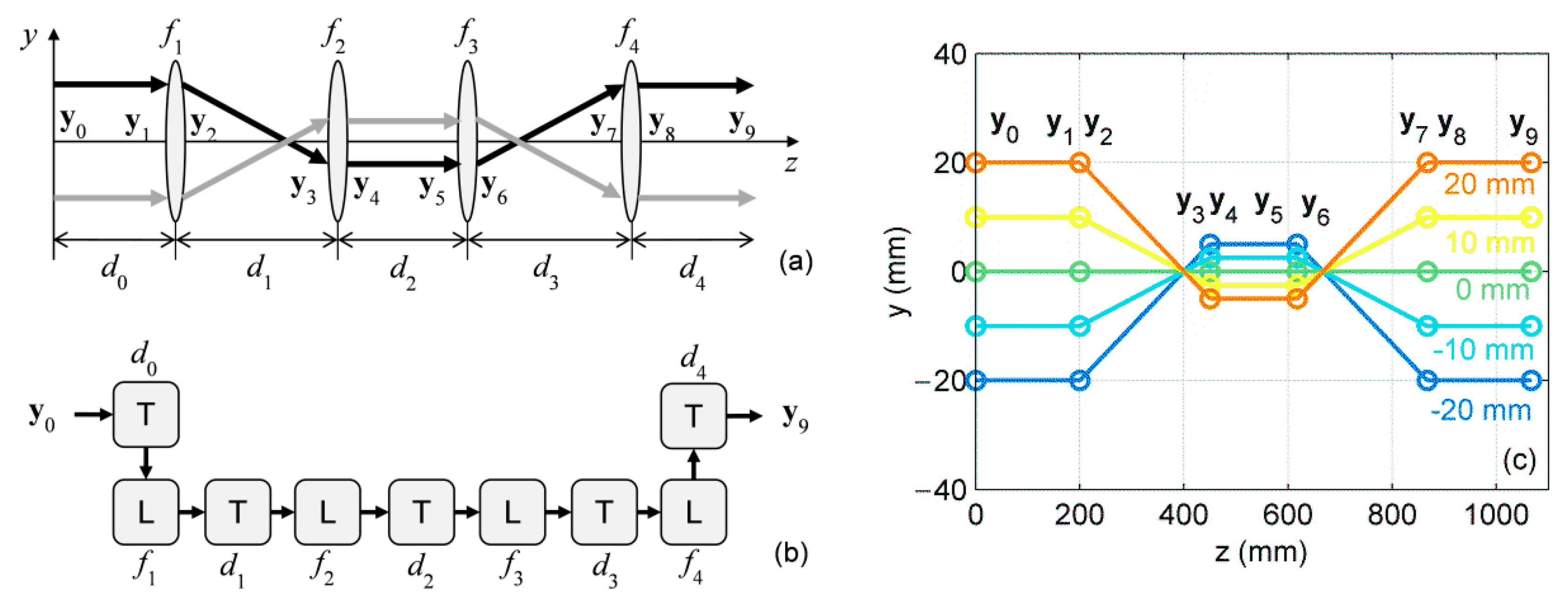
4.1. Paraxial Cloaking

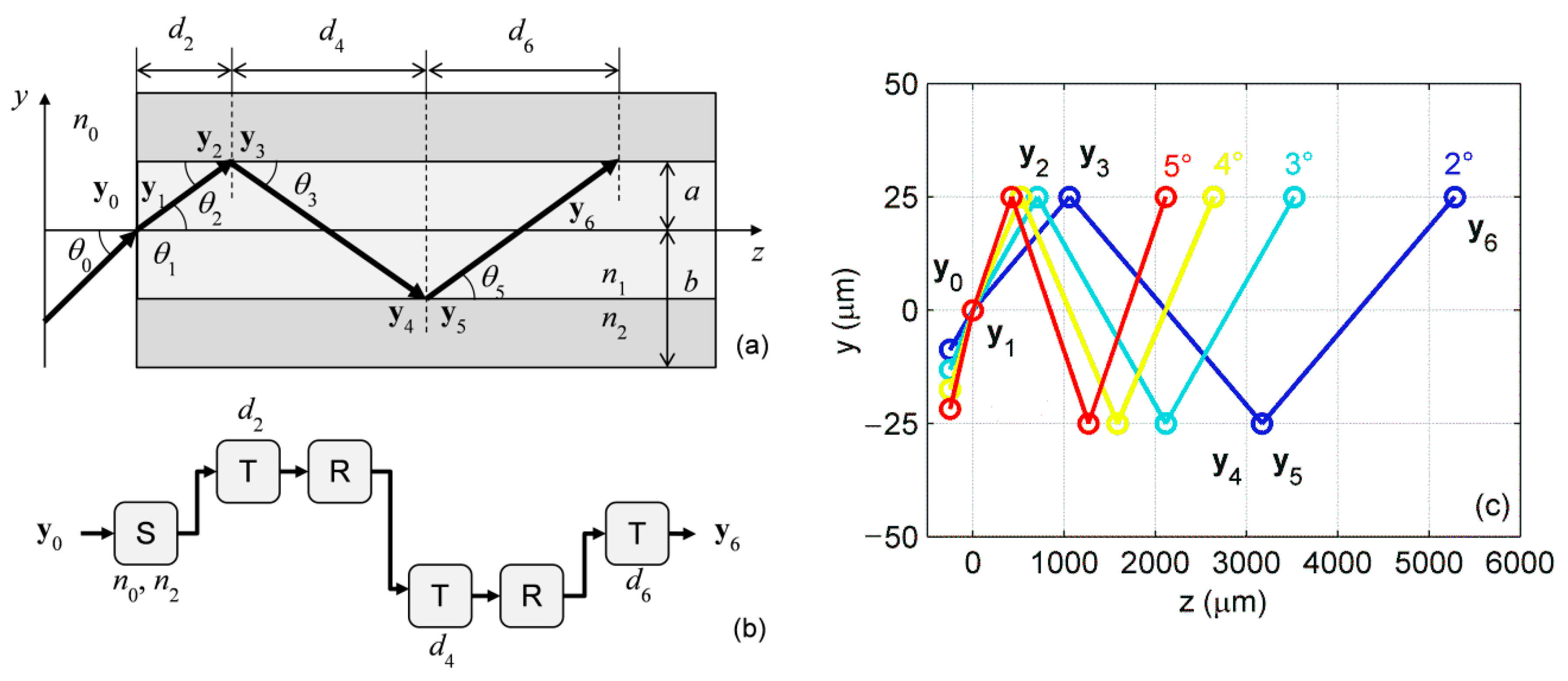
Paraxial optical cloaking [23] is an ingenious application of geometrical optical design. If the overall ray transfer matrix is equivalent to the transmission through a constant refractive index medium, regions enclosed by the system optics are perfectly cloaked, and objects placed inside these spaces do not affect the output light, becoming invisible. Such a condition is achieved with a four-lenses setup, Figure 3a, in which focal lengths and path distances must satisfy d₁ = f₁ + f₂ and d₂ = 2f₂ (f₁ + f₂)/(f₁ − f₂) for f₁ = f₄, f₂ = f₃, and d₁ = d₃.

The system model is implemented using eight optical elements as depicted in Figure 3b, assuming 50 mm diameter, thin lenses for the sake of simplicity. As proposed in [23], for f₁ = f₄ = 200 mm and f₂ = f₃ = 50 mm, distances d₁ = d₃ and d₂ must be 250 and ~167 mm, respectively. For visualization purposes, the model also includes free-space transmissions of length d₀ = d₄ = 200 mm for input and output rays. Static simulations carried out by scanning the input height within −20 ≤ y₀ ≤ 20 mm provides the ray tracing profile shown in Figure 3c, which evidences the cloaked region for 200 ≤ z ≤ 800 mm. As the rays are vertically confined to −5 ≤ y₀ ≤ 5 mm, objects strategically placed between lenses f₁ and f₄ do not block the passage of light, i.e., y₈ and θ₈ remain unchanged in relation to y₁ and θ₁, respectively, and the optical system approximates a transmission element. Results are comparable to the ray tracing simulations conducted with CODE V software depicted in [23], but differ because the latter uses achromatic doublets instead of thin lenses and also computes aberrations. Nevertheless, function blocks can be simply permuted in the system model to simulate practical optical elements and achieve a more realistic analysis.

4.2. Optical Fiber

In an optical fiber, light travels through the core region and confined by total internal reflection (TIR) at the core-cladding interface. Transmission in multimode fibers can be treated by geometrical optics approach [24]; despite its simplicity, such model is useful for demonstrating basic concepts such as the effect of fiber geometry and material on light coupling and transmission [25], estimating waveguide losses [26], and modeling fiber sensors [27].

Consider a fiber with core and cladding radii a and b, respectively, wherein refractive indices of surrounding medium, core, and cladding are n₀, n₁, and, n₂, respectively, as illustrated in Figure 4a. Input light refracts at the air-core interface (n₀ < n₁) and travels in the yz-plane as a meridional ray with orientation θ₁ = θ₂ along the distance d₂ = a/θ₁ (skewed rays are neglected in this model) until it reaches the core-cladding boundary (n₁ > n₂). In the case of total internal reflection, light is totally reflected with θ₃ = −θ₂ and confined inside the core with consecutive transmissions along with d₄ = 2a/θ₃ and d₆ = 2a/θ₅. The TIR condition is only achieved if the orientation of input ray θ₁ is smaller than a maximum entrance angle θ_i, where NA = n₀ sin θ_i = (n₁² − n₂²)^1/2, NA is called the fiber numerical aperture [24].

The implemented model is shown in Figure 4b assuming only two reflections for clarity, with y₀ = 0 and 2° ≤ θ₀ ≤ 5°. As the core-cladding interface is parallel to z-axis, the reflection ABCD matrix must be adjusted to D = −1 to correct the orientation of output light. Even though rays refracted into the cladding violate the paraxial approximation, the TIR condition can be verified by testing if θ₂ ≤ θ_max = π/2 − θ_c, where θ_c = sin⁻¹(n₂/n₁) is the critical angle [24]. Static simulations were conducted with a = 25 µm, b = 62.5 µm, n₀ = 1, n₁ = 1.475, and n₂ = 1.460, so the fiber numerical aperture is NA = 0.21, yielding θ_i = 12.11° and θ_max ≈ 8.18°, corroborating the analytical model. Ray tracing results for different orientations are plotted in Figure 4c, for example, θ₀ = 5° produces θ₂ = 3.39°, satisfying the TIR. Besides, the fact of the light rays experience particular traveling times through the fiber is useful to introduce the modal dispersion among low-order and high-order modes, i.e., rays propagating straight or at steeper angles, respectively. Such a phenomenon is the limiting factor in the information transmission capacity of multimode fiber systems and results in a high bandwidth-distance product value [24].

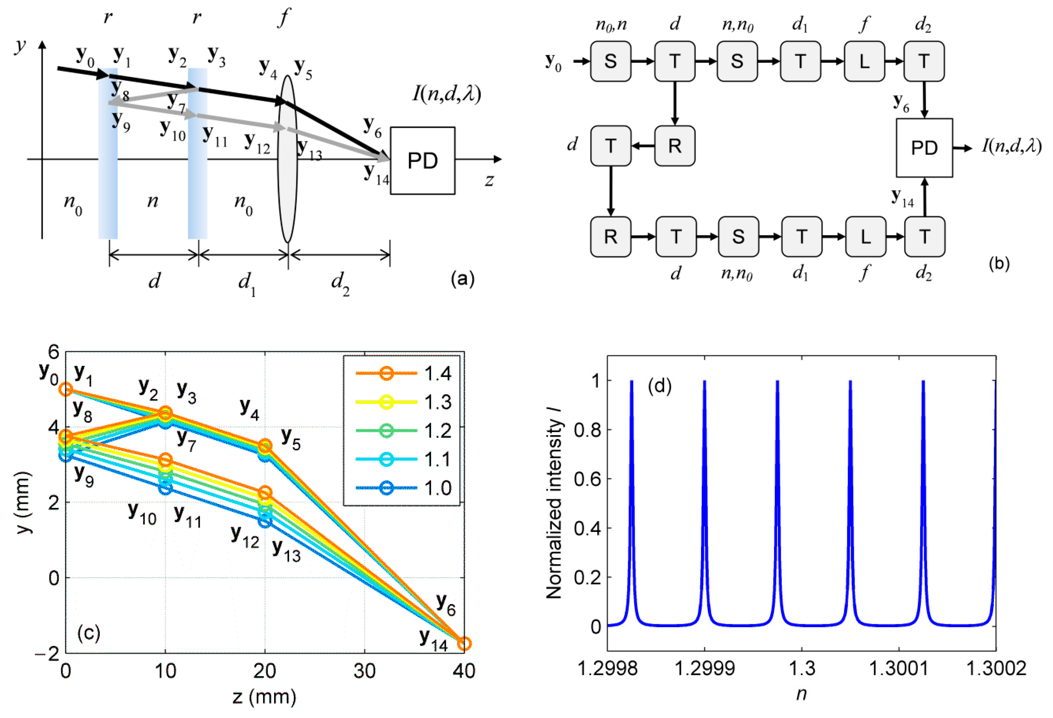
4.3. Fabry–Perot Interferometer

A typical Fabry–Perot interferometer (FPI) is comprised of a pair of planar mirrors with reflectivity r that traps the incident ray (orientation θ₀) inside a cavity of length d and refractive index n, promoting successive reflections as shown in Figure 5a. The light transmitted by the mirror is collected with a thin lens and focused on a photodetector for assessing the output light intensity I. Interference cannot be evaluated merely by geometrical optics; alternatively, one may determine the light confinement using ray tracing and calculate I by wave optics approach,

$$I=\frac{I_0/{\left(1-r\right)}^2}{1+{\left(2F/\pi \right)}^2\sin (\varphi /2)}$$

(2)

I₀ is the input intensity, F = π r^1/2/(1 − r) is the resonator finesse, and φ = 4πnd/λ is the phase difference, where λ is the wavelength [22]. The high sensitivity to n, d, and λ makes the FPI applicable for chemical and displacement sensing [28], as well as an optical filter or spectrum analyzer [29].

The FPI surrounded by the air (n₀ = 1.00) is modeled as depicted in Figure 5b, neglecting the thickness of mirrors and using a thin lens with f = 20 mm. Distances are set to d₁ = 10 mm and d₂ = 20 mm. To investigate that the effect of the cavity refractive index n, simulations are carried out with r = 0.9, λ = 1 μm, d = 10 mm, and 1.00 ≤ n ≤ 1.40. Ray tracing results with y₀ = 5 mm and θ₀ = −5°, Figure 5c, indicate that the incident light undergoes multiple reflections inside the cavity while the output paraxial rays are appropriately focused on the observation plane of the photodetector, as predicted by the analytical model. Moreover, scanning the FPI response for different n reveals the expected normalized intensity profile. Analogous tests could be performed to examine the contribution of d or λ. Furthermore, this study suggests that optics models belonging to different approaches can be coupled using the modular strategy and run into a unique simulation environment.

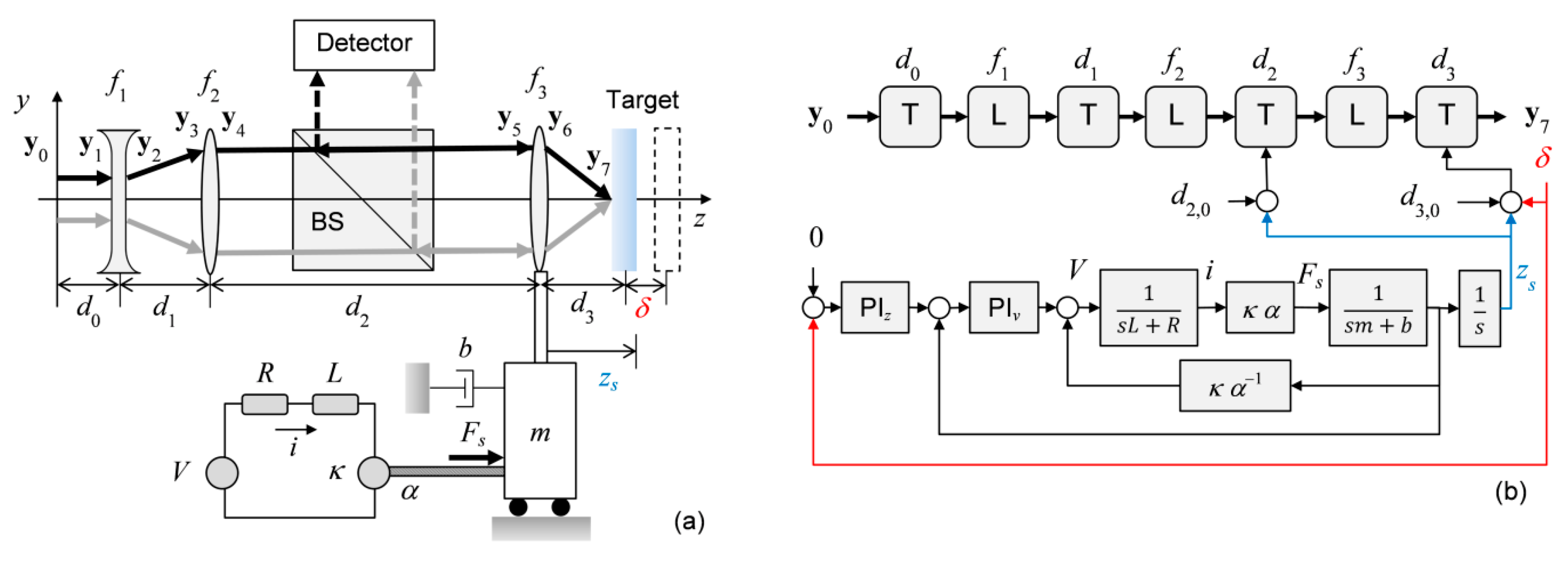
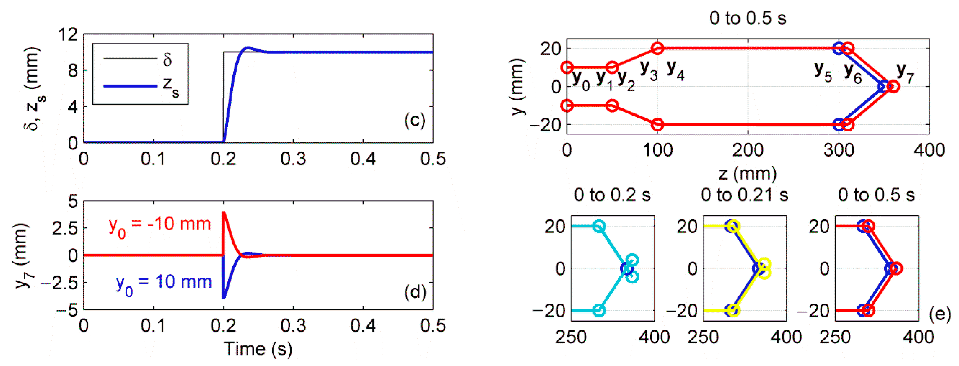
4.4. Automatic Focusing System

Ultimately, to demonstrate the application of the ray optics model in a multi-domain simulation, an automatic focusing system is designed, as shown in Figure 6a. This setup is analogous to an optical pickup head used in disk readers: the input beam emitted by a laser source is expanded (f₁), collimated (f₂), and then focused with an objective lens (f₃) at the surface of a reflective target, whereas the reflected light is further directed to the photodetector by a beam splitter (BS) [5]. If the target displaces along z-direction by δ, the position of the objective lens must be compensated to keep the beam focused, which can be accomplished by a translational stage driven by servo motor that moves the lens along the z-axis. Besides its traditional application, prospective uses for this system encompass mechanical sensors [30] and tweezers for single-cell trapping [31].

The system is modeled by a set of three thin lenses, Figure 6a. Although the optics for light detection is not considered for simplicity, it is presumed that the distance between the objective and the target surface d₃ is estimated from the photodetector signal. The objective is mounted on the motorized stage and displaced by z_S. The linear actuator is modeled as a permanent-magnet DC motor (armature resistance R and inductance L, electrical constant κ, and mechanical coupling ratio α) that produces a force F_S required to move the working load (equivalent mass m and damping b). The servo system is implemented by proportional-integral (PI) controllers forming an internal velocity loop and an outer position loop (current controller and electric motor drive are omitted). Therefore, if the target is displaced by δ, the position of the objective must be compensated by d₂ = d_2,0 + z_S and d₃ = d_3,0 + δ − z_S to adjust the focus, where d_2,0 and d_3,0 are the initial path lengths and z_S is set by the electromechanical servo control.

Simulations are carried out according to the block diagram depicted in Figure 6b, using Runge-Kutta solver and time step of 10⁻⁵ s. Optical system is built with d₀ = d₁ = d_3,0 = 50 mm, d_2,0 = 200 mm, f₁ = −50 mm, f₂ = 100 mm, and f₃ = 50 mm. The motor has R = 33 Ω, L = 0.6 mH, rated voltage of 6 V, and rated speed of 2.3 mm/s, yielding κ = 2.6 × 10³ V.s/mm [32], whereas the linear stage has m = 0.3 kg, b = 0.02 N.s/m, and α = 10³. Initially, the electromechanical system is simulated separately for tuning the PI controllers to achieve a rise time <0.1 s, stationary error <1%, and guarantee a speed controller (inner loop) faster than the position one (outer loop). Subsequently, the optical model is coupled with the system mechanics for evaluating the focus correction.

As shown in Figure 6c, for the system disturbed with an abrupt displacement of 10 mm at 0.2 s, the linear stage position signal z_S follows δ to correct the distance d₃ and compensate d₂. Monitoring the height y₇ of output ray y₇, Figure 6d, indicates that the light is initially deviated at 0.2 s due to δ, then the control loop adjusts y₇ to 0 (focusing on the target surface) in less than 0.1 s with a negligible steady-state error. Ray tracing for y₀ = ±10 mm and θ₀ = 0 is presented in Figure 6e at 0 s (initial condition, similar to the depicted in [5]), 0.2 s (disturbance), 0.21 s (regulation), and 0.5 s (final position), wherein the automatic focus is evidenced: firstly, the target departs from its original position and defocus the light, then, the objective moves toward +z until the height of output rays become zero, indicating that the focus was restored.

The modular project allows for refining or changing the controllers to enhance the system performance, whereas the electrical and mechanical modules can be replaced by more realistic approaches to meet the implementation requirements. Another possible application is the design of three lenses zoom system, in which one lens is fixed, whereas the other two elements are moved to adjust the focal length (magnification) without changing the image plane [33]. The strict requisites of settling time and overshoot demand sophisticated control strategies for displacing the two lenses simultaneously [34]; therefore, the proposed model-based design tool is convenient for implementing control loops and evaluating the results in terms of ray tracing through a unique simulation environment.

5. Conclusions

The model-based design was validated as a useful tool to build and simulate paraxial optics systems from pure-optical to multi-domain optomechatronics projects. Ray tracing can be combined with dynamic simulations to move lenses and mirrors and perform precise focus control. Moreover, multiple rays as in resonators can be split into branches and computed simultaneously. Therefore, starting from a very basic model, students and professionals can integrate several subsystems to upgrade their simulation and achieve practical and realistic analyses, whereas the modular approach allows for exchanging parts of the system to update its functionalities without modifying the overall project.

Despite the promising results, this methodology is currently restricted to paraxial geometrical optics models, i.e., extreme bending of light rays will probably yield inaccurate tracing, whereas important phenomena, such as diffraction, interference, and attenuation, cannot be represented with this proposal so that eventual deviations may occur regarding the experimental realization of the optical systems. Besides, most commercial, dedicated solutions integrate wave and Gaussian optics simulations with the ray tracing analyses, which is crucial for the optimization of optical systems. Nevertheless, one can develop blocks for non-paraxial optical elements, as well as additional functions for establishing an interface between ray and wave optics. Further studies will focus on such improvements to create a more versatile, simple, and feasible multi-domain environment for simulating optical systems.

References

1. Cabrera, A.A.A.; Foeken, M.J.; Tekin, O.A.; Woestenenk, K.; Erden, M.S.; De Schutter, B.; van Tooren, M.J.L.; Rabuška, R.; van Houten, F.J.A.M.; Tomiyama, T. Towards automation of control software: A review of challenges in mechatronic design. Mechatronics 2010, 20, 876–886. [Google Scholar] [CrossRef]
2. Gamo, J. Assessing a virtual laboratory in optics as a complement to on-site teaching. IEEE Trans. Educ. 2019, 62, 119–126. [Google Scholar] [CrossRef]
3. Verlage, E.; Saini, S.; Agarwal, A.; Serna, S.; Kosciolek, R.; Morrisey, T.; Kimerling, L.C. Web-based interactive simulations and virtual lab for photonics education. In Proceedings of the Fifteenth Conference on Education Training in Optics and Photonics (ETOP 2019), Quebec City, QC, Canada, 21–24 May 2019; OSA: Washington, DC, USA, 2019; p. 11143_136. [Google Scholar] [CrossRef]
4. Sanchez del Rio, M.; Canestrari, N.; Jiang, F.; Cerrina, F. SHADOW3: A new version of the synchrotron X-ray optics modelling package. J. Synchrotron Radiat. 2011, 18, 708–716. [Google Scholar] [CrossRef] [PubMed] [Green Version]
5. Cohen, D.K.; Gee, W.H.; Ludeke, M.; Lewkowicz, J. Automatic focus control: The astigmatic lens approach. Appl. Opt. 1984, 23, 565–570. [Google Scholar] [CrossRef] [PubMed]
6. Logozzo, S.; Valigi, M.C.; Canella, G. Advances in optomechatronics: An automated tilt-rotational 3D scanner for high-quality reconstructions. Photonics 2018, 5, 42. [Google Scholar] [CrossRef] [Green Version]
7. Cho, H.; Kim, M.Y. Optomechatronic technology: The characteristics and perspectives. IEEE Trans. Ind. Electron. 2005, 52, 932–943. [Google Scholar] [CrossRef]
8. Knight, J.S.; Acton, D.S.; Lightsey, P.; Barto, A. Integrated telescope model for the James Webb space telescope. In Proceedings of the SPIE Astronomical Telescopes + Instrumentation, Proceedings of SPIE 8449, Amsterdam, The Netherlands, 1–6 July 2012; SPIE: Bellingham, WA, USA, 2012; p. 84490V. [Google Scholar] [CrossRef]
9. Wittkopf, S.; Grobe, L.O.; Geisler-Moroder, D.; Compagnon, R.; Kämpf, J.; Linhart, F.; Scartezzini, J.-L. Ray tracing study for non-imaging daylight collectors. Sol. Energy 2010, 84, 986–996. [Google Scholar] [CrossRef]
10. González, G.D.; Castillo, M.D.I. Model of the human eye based on ABCD matrix. In Proceedings of the 6th Ibero-American Conference on Optics/9th Latin-American Meeting on Optics, Lasers and Applications, AIP Conference Proceedings 992, Campinas, Brazil, 21–26 October 2007; AIP: Melville, NY, USA, 2007; pp. 108–113. [Google Scholar] [CrossRef]
11. Parker, S.G.; Bigler, J.; Dietrich, A.; Friedrich, H.; Hoberock, J.; Luebke, D.; McAllister, D.; McGuire, M.; Morley, K.; Robinson, A.; et al. OptiX: A general purpose ray tracing engine. ACM Trans. Graph. 2010, 29, 66. [Google Scholar] [CrossRef]
12. Osório, T.; Horta, P.; Larcher, M.; Pujol-Nadal, R.; Hertel, J.; van Rooyen, D.W.; Heimsath, A.; Schneider, S.; Benitez, D.; Frein, A.; et al. Ray-tracing software comparison for linear focusing solar collectors. In Proceedings of the International Conference on Concentrating Solar Power and Chemical Energy Systems, AIP Conference Proceedings 1734, Cape Town, South Africa, 13–16 October 2015; AIP: Melville, NY, USA, 2016; p. 020017. [Google Scholar] [CrossRef] [Green Version]
13. Mauch, F.; Gronle, M.; Lyda, W.; Osten, W. Open-source graphics processing unit-accelerated ray tracer for optical simulation. Opt. Eng. 2016, 52, 053004. [Google Scholar] [CrossRef] [Green Version]
14. Savage, N. Optical design software. Nat. Photonics 2007, 1, 598–599. [Google Scholar] [CrossRef]
15. Poon, T.-C.; Kim, T. Engineering Optics with MATLAB; World Scientific Publishing: Hackensack, NJ, USA, 2006. [Google Scholar]
16. Anterrieu, E.; Perez, J.-P. MOTO: A Matlab object-oriented programming toolbox for optics. In Proceedings of the Education Training in Optics and Photonics, Ottawa, ON, Canada, 3 June 2007; OSA: Washington, DC, USA, 2007; p. ETD3. [CrossRef]
17. Crowther, B.G.; Wassom, S.R. Toward end-to-end optical system modeling and optimization: A step forward in optical design. In Proceedings of the Optical Science and Technology, the SPIE 49th Annual Meeting, Proceedings of SPIE 5524, Denver, CO, USA, 2–6 August 2004; SPIE: Bellingham, WA, USA, 2004; pp. 196–204. [Google Scholar] [CrossRef]
18. Wilson, W.C.; Atkinson, G.M. MOEMS Modeling Using the Geometrical Matrix Toolbox, NASA Technical Reports Server. 2005. Available online: https://ntrs.nasa.gov/search.jsp?R=20050237975 (accessed on 12 October 2020).
19. Tarsaria, H.; Alvarenga, J.; Desai, A.; Rad, K.; Boussalis, H. Ray tracing visualization using LabVIEW for precision pointing architecture of a segmented reflector testbed. In Proceedings of the 19th Mediterranean Conference on Control & Automation, Corfu, Greece, 20–23 June 2011; IEEE: Bellingham, WA, USA, 2011; pp. 1367–1372. [Google Scholar] [CrossRef]
20. Delano, E. First-order design and the y, ӯ diagram. Appl. Opt. 1963, 12, 1251–1256. [Google Scholar] [CrossRef]
21. Schwab, M.; Herkommer, A. The Delano diagram, a powerful design tool. In Proceedings of the Optical Systems Design, Proceedings of SPIE 7100, Glasgow, Scotland, UK, 2–5 September 2008; SPIE: Bellingham, WA, USA, 2008; p. 71000U. [Google Scholar] [CrossRef]
22. Saleh, B.E.A.; Teich, M.C. Fundamentals of Photonics; John Wiley & Sons: New York, NY, USA, 1991. [Google Scholar]
23. Choi, J.S.; Howell, J.C. Paraxial ray optics cloaking. Opt. Express 2014, 22, 29465–29478. [Google Scholar] [CrossRef] [PubMed] [Green Version]
24. Keiser, G. Optical Fiber Communications; McGraw-Hill: New York, NY, USA, 1991. [Google Scholar]
25. Snyder, A.W.; Pask, C.; Mitchell, D.J. Light-acceptance property of an optical fiber. J. Opt. Soc. Am. 1973, 63, 59–64. [Google Scholar] [CrossRef] [PubMed]
26. Tekelioglu, M.; Wood, B.D. Prediction of light-transmission losses in plastic optical fibers. Appl. Opt. 2005, 44, 2318–2326. [Google Scholar] [CrossRef]
27. Lomer, M.; Arrue, J.; Jauregui, C.; Aiestaran, P.; Zubia, J.; López-Higuera, J.M. Lateral polishing of bends in plastic optical fibres applied to a multipoint liquid-level measurement sensor. Sens. Actuators A Phys. 2007, 137, 68–73. [Google Scholar] [CrossRef]
28. Beard, P.C. Interrogation of free-space Fabry-Perot sensing interferometers by angle tuning. Meas. Sci. Technol. 2003, 14, 1998–2005. [Google Scholar] [CrossRef] [Green Version]
29. Jovanov, V.; Bunte, E.; Stiebig, H.; Knipp, D. Transparent Fourier transform spectrometer. Opt. Lett. 2011, 36, 274–276. [Google Scholar] [CrossRef]
30. Chu, C.-L.; Lin, C.-H. Development of an optical accelerometer with a DVD pick-up head. Meas. Sci. Technol. 2005, 16, 2498–2502. [Google Scholar] [CrossRef]
31. Kasukurti, A.; Potcoava, M.; Desai, S.A.; Eggleton, C.; Marr, D.W.M. Single-cell isolation using a DVD optical pickup. Opt. Express 2011, 19, 10377–10386. [Google Scholar] [CrossRef]
32. Thorlabs. Z8 Series Motorized DC Servo Actuators—User Guide. 2018. Available online: www.thorlabs.com/thorproduct.cfm?partnumber=Z825B (accessed on 13 October 2020).
33. Yue, M.S.; Shiue, S.-G.; Lu, M.-H. Two-optical-component method for designing zoom system. Opt. Eng. 1995, 34, 1826–1834. [Google Scholar] [CrossRef]
34. Wick, D.V.; Martinez, T. Adaptative optical zoom. Opt. Eng. 2004, 43, 8–9. [Google Scholar] [CrossRef]
Figure 1. Modeling optical systems: (a) matrix optics notation; (b) expanded transfer matrix; (c) concatenated optical elements.
Applsci 10 08278 g001
Figure 2. Modeling refraction and reflection between two media of refractive indices n1 and n2: (a) ray optics representation; (b) transfer matrix model; and (c) implementation in MATLAB Simulink.
Applsci 10 08278 g002
Figure 3. Paraxial cloaking: (a) ray optics representation (adapted from [23]); (b) matrix optics model, T and L are transmission and thin lens components, respectively; (c) ray tracing obtained by simulation for −20 ≤ y0 ≤ 20 mm and θ0 = 0°, cloaked region is evidenced for 200 ≤ z ≤ 800 mm.
Applsci 10 08278 g003
Figure 4. Transmission through multimode optical fiber: (a) ray optics representation; (b) matrix optics model, S is refraction and R is reflection component; (c) ray tracing obtained by simulation for y0 = 0 and 2° ≤ θ0 ≤ 5°.
Applsci 10 08278 g004
Figure 5. Fabry–Perot interferometer: (a) ray optics representation where PD is a photodetector (multiple reflections are omitted for clarity); (b) matrix optics model and block diagram; (c) ray tracing obtained by simulation for y0 = 5 mm, θ0 = −5°, and 1.00 ≤ n ≤ 1.40 (refractive index values in the legend); and (d) normalized intensity around n = 1.30.
Applsci 10 08278 g005
Figure 6. Optical pickup head with automatic focus control: (a) ray optics and mechatronics representation (adapted from [5]); (b) matrix optics model and block diagram, PIz and PIv are position and speed controllers, respectively, and s is the Laplace variable; effect of focus compensation on (c) displacement zS and (d) ray height y7; and (e) ray tracing obtained by simulation for y0 = ±10 mm and θ0 = 0, the bottom plots show the output beam position at different times.
Applsci 10 08278 g006aApplsci 10 08278 g006b