Article

Automatic Extraction of Material Defect Size by Infrared Image Sequence

1
Key Laboratory of Nondestructive Testing (Ministry of Education), Nanchang Hangkong University, Nanchang 330063, China
2
Department of Computer Science, Birmingham City University, Birmingham B5 5JU, UK
3
School of Computer Science and Technology, Harbin Engineering University, Harbin 150001, China
4
Defence Academy of United Kingdom, Cranfield University, Shrivenham, Swindon SN6 8LA, UK
5
Department of Computer Science, Edge Hill University, Ormskirk L39 4QP, UK
*
Author to whom correspondence should be addressed.
Appl. Sci. 2020, 10(22), 8248; https://doi.org/10.3390/app10228248
Submission received: 5 November 2020 / Revised: 16 November 2020 / Accepted: 17 November 2020 / Published: 20 November 2020
(This article belongs to the Special Issue Infrared Imaging and NDT)

Abstract

:
A typical pulsed thermography procedure results in a sequence of infrared images that reflects the evolution of temperature over time. Many features of defects, such as shape, position, and size, are derived from single image by image processing. Hence, determining the key frame from the sequence is an important problem to be solved first. A maximum standard deviation of the sensitive region method was proposed, which can identify a reasonable image frame automatically from an infrared image sequence; then, a stratagem of image composition was applied for enhancing the detection of deep defects in the key frame. Blob analysis had been adopted to acquire general information of defects such as their distributions and total number of defects. A region of interest of the defect was automatically located by its key frame combined with blob analysis. The defect information was obtained through image segmentation techniques. To obtain a robustness of results, a method of two steps of detection was proposed. The specimen of polyvinyl chloride with two artificial defects at different depths as an example was used to demonstrate how to operate the proposed method for an accurate result. At last, the proposed method was successfully adopted to examine the damage of carbon fiber-reinforced polymer. A comparative study between the proposed method and several state-of-the-art ones shows that the former is accurate and reliable and may provide a more useful and reliable tool for quality assurance in the industrial and manufacturing sectors.

1. Introduction

The health monitoring of materials and structures plays a vital role in the fields of aerospace, industry, medical, and construction [1,2]. In many major projects, even minor material defects may cause major hidden danger. Therefore, nondestructive testing (NDT) technology provides a strong technical guarantee for the safety of material structure. As a new nondestructive testing technology, pulsed thermal nondestructive testing (TNDT) is widely used in the detection of defects in materials and structures due to its large detection area, fast detection speed, detection convenience, and cheap equipment [3]. Researchers can obtain the continuous change process of the transient temperature field on the material surface through the infrared thermal imager. A sequence of infrared images expresses the evolution of temperature intuitively. The method of digital image processing is applied to assess and analyze the information of the defect quantitatively such as the location, shape, and size of the defect. To quantify the size of defects has been one of the most critical processes in the infrared-based nondestructive defect detection. It is the deterministic factor for the acceptance or rejection of the specimen during the quality control process. Despite the popularity for using the thermographic technique as an efficient method for defect detection, there are still a number of outstanding issues that are under active research.
First of all, an inspector needs to select the frame that best represents the material defect information from hundreds of infrared images. There are rare research studies on the qualitative index of frame number selection at present. Generally, this had been proceeded through the identification of the image frames that exhibited substantial surface temperature contrast between the defect area and the sound region [4]. There is an element of subjectivity in these approaches. Tashan et al. [5] pointed out that the quantification of the defect size was critically dependent on the selection of the appropriate time frame of the thermogram for defect evaluations. It was concluded that in order to obtain a more accurate dimensions of the defect, it was necessary to analyze the infrared thermal image with the largest temperature difference contrast or immediately thereafter by analyzing the defect results at different distances and inspection times. Kabouri A. et al. [6] selected the frames that depicted the largest average surface temperature of the specimen as the candidate image frame data. However, the robustness of the image frame sequence selection methodology has been shown to be generally poor, and the proposed method of selecting an infrared sequence key frame has poor accuracy in the final defect extraction.
In the next place, raw images are usually not suitable for accurate material assessment [7]. In order to further obtain the defect information of the material damage, the image needs to be digitally processed. However, the contrast of infrared images is commonly low and normally accompanied with significant blurred edges, especially those associated with structural defects such as cracks [8,9]. A number of factors such as uneven heating, precision of the equipment, electro-magnetic radiation (emission) from the background etc. are the main contributions that reduce the contrast of the thermogram significantly [10,11]. Undoubtedly, this is an additional challenge to the qualitative and quantitative identification and evaluation of defects especially when the thermographic technique is employed for the NDE. There have been two main ways for processing infrared images: the non-uniformity correction method [12,13,14] and the detailed enhancements of infrared images. Hansan [15] pointed out that the median filter had better edge retention characteristics on the basis of noise removal capability particularly when imagery contains the edge feature of the defects. Meanwhile, on the basis of keeping the size of the defect area unchanged, morphological opening operation that smoothens the boundary of the defect and eliminates small spikes has been reported. Wang [16] applied the Levenberg–Marquardt iterative algorithm for denoising, thereby improving the contrast of the thermal data. More recent work has been using bionic intelligence algorithms for denoising and then the edge detection of defect features through the ant colony algorithm [17] after the time derivative profile is polynomial fitted. A more advanced hybrid method that integrates the simulation annealing algorithm (SA) and Nelder–Mead simplex search method (NM) for the quantification of the sizes and depths of subsurface defects of the carbon fiber-reinforced plastic (CFRP) laminate materials has also been attempted with good results [18]. Grys [19] showed that the error for defining the defect boundaries followed the finite spatial resolution of the numerical model in the Otsu’s segmentation method is rather significant. Sreeshan [20] adopted the watershed technique and Gabor filtering to detect defects, and good results have been obtained. Furthermore, there are a number of image segmentation techniques available for the quantitative recognition of defects, e.g., the iterative threshold method, the maximum entropy method, the minimum error method, the Otsu method, and the minimum deviation method; however, none of them is capable of extracting defect features automatically without the need for operator intervention. Although the Otsu method has been shown to be more capable of extracting defects even for those in different depths [21], it still cannot realize the extraction of defect features automatically.
Feature extraction is another critical step in the image based on NDE for defect detection. There are two main approaches that have been used for the quantitative detection of defect size: (i) the analysis of the surface temperature field data and (ii) through the digital processing of the image data. One of the most classical ways for the quantitative assessment of defect dimensions and the extraction of the defect temperature profile is using the Wetsel and McDonald’s temperature field analysis method through the full width at half maxima (FWHM) of the defect feature [22]. This is still a popular method being used for defects characterization [23,24]. Olga [25] improved the method by using the time derivative of the surface temperature distribution to determine the defect size through the half-height tangent method. Duan [26] demonstrated the use of the signal to noise ratio (SNR) analysis of the temperature distribution profile for the assessment of physical property of defects: when the SNR of the observed thermal anomaly is larger than 15, then the feature is considered as induced by defects. In the second approach of defects analysis which focuses more on digital processing of infrared images, a sparse principal component thermography (SPCT) method had been proposed to enhance the contrast of the defect induced thermal anomaly with respect to the background and the noise of the imaging sensor [27]. At present, the most mainstream method of defect representation (area) is still using the equivalent pixel ratio method [5,6], which estimates the defect area through the number of image pixels of the defect image. The equivalent length ratio for each pixel can be calibrated by using the known dimension of the specimen.
Based on the outstanding issues as outlined above, this work attempts to address the automatic selection of suitable image frames from an infrared image sequence for processing and to characterize the defects of the material robustly and accurately under the long pulse thermographic experimental configuration. The workability of the proposed method is demonstrated by the detection of artificial defects in polyvinyl chloride (PVC), and the feasibility and accuracy of this method are verified by the impact damage detection of carbon fiber-reinforced plastics (CFRP).

2. Theory and Methods

2.1. Principle of Long Pulse Thermography

In the application of pulsed infrared nondestructive testing, the heat diffusing across a media is susceptible to the property of the media as well as to environmental factors. In the Cartesian coordinates, the transient temperature T (x, y, z) is in an unsteady state, and in the absence of an internal heat source, it is a function of space and time. For an arbitrary interface S with a corresponding volume V in the media (see Figure 1a,b), the temperature gradient in the normal direction of a small element on the closed surface of S can be written as follows:
T n = T x cos α + T y cos β + T z cos γ
where α, β, and γ are the angles between the normal vector n and the X-axis, Y-axis, and Z-axis, respectively. According to the Fourier law, the heat flows through the dS in unit time can be expressed by:
q = λ [ T x cos α + T y cos β + T z cos γ ] d S
where λ is the thermal conductivity of the media (W/(m·K)). The double integral is computed based on the above formula and it is then converted into triple integral as follows:
Q = V λ [ x ( T x ) + y ( T y ) + z ( T z ) ] .
In contrast, according to the basic concept of heat conduction, the total amount of heat contained in the volume V is:
Q V = V c ρ T ( x , y , z , τ ) d V
where c is the specific heat capacity of infinitesimal (J/(kg·°C)), and ρ is the density of infinitesimal (kg/m3). The diffusion of T over the volume V per unit time is:
q V = V c ρ T τ d V .
Equations (3) and (5) are different mathematical forms of the same physical quantity, leading to the following equation:
c ρ T τ = λ ( x ( T x ) + y ( T y ) + z ( T z ) ) .
Therefore, the three-dimensional unsteady heat conduction differential equation becomes:
2 T ( x , t ) x 2 + 2 T ( y , t ) y 2 + 2 T ( z , t ) z 2 = 1 α T ( x , t ) t
where T (x, t) is the temperature of the spot x at the time t and it is a property of the coefficient of thermal diffusivity that has been used for measuring the heat transfer and storage ability of the material. Equation (7) gives the form of three-dimensional heat transfer (diffusion) function. It is generally difficult to find the analytical solution because of the complexity of the actual solution conditions. Therefore, this equation is often simplified to the form of one-dimensional heat conduction in practice. While the one-dimensional heat conduction theory cannot explain all the thermal phenomena, the one-dimensional heat conduction model derived from the heat transfer differential equations can provide approximate solution to problems [28] in most of our experiments (such as thickness measurement). Under given initial boundary conditions, the function of thermal energy propagating in the medium can be obtained by solving the heat conduction equation.
Now, suppose a sheet of isotropic material with a thickness of x2 along the x-axis direction, as shown in Figure 1c. At the lower part of the sheet is a pit defect x1 deep from the surface. Assume that the temperature is uniform across the cross-section perpendicular to the x-axis, which means that there is no heat exchange between the sheet and the ambient environment and there is no heat source in the bulk of the sheet material. When the specimen is excited by a heat pulse Q which is then absorbed by the object surface, the transient temperature of the specimen varies as a function of the coordinates x and time t according to the heat diffusion equation:
2 T ( x , t ) x 2 = 1 α T ( x , t ) t
where α is the thermal diffusivity. To simplify the calculation, α can be regarded as a constant.
Heat is applied to the surface of the test object at t = 0. Assuming at T (x, 0), the energy absorbed by the object surface is Q; then, the heat transfer Equation (8) at any position x 0 is solved as:
T ( x , t ) = Q 2 α π t e x p ( x 2 4 α t ) .

2.2. Maximum of Sandard Deviation of Sensitive Region Method (MSDSRM)

Equation (9) indicates that the propagation of the Q can be affected by the presence of defects in the bulk of the material, and that different defects at different depths would have different character times for affecting the distribution of temperature of specimen at the surface. When it happens, the rate of heat diffusion into the bulk of the specimen is perturbed by the presence of defects, and this manifests as a gradual emerging and then disappearing of heat as a function of time. When the object is monitored by a heat sensor such as a thermal camera, the time frame of the thermal images will be a good indicator for pinpointing the physical location of the defects inside the bulk of the specimen. Therefore, the selection of a appropriate image frames from the thermographic image sequence will allow one to assess the shapes and areas of different defects at different depths readily. However, the key issue for the identification of a suitable frame from thousands of infrared frame sequence seems to be non-trivial. Consider there is one subsurface defect in the simplistic example, as shown in Figure 2.
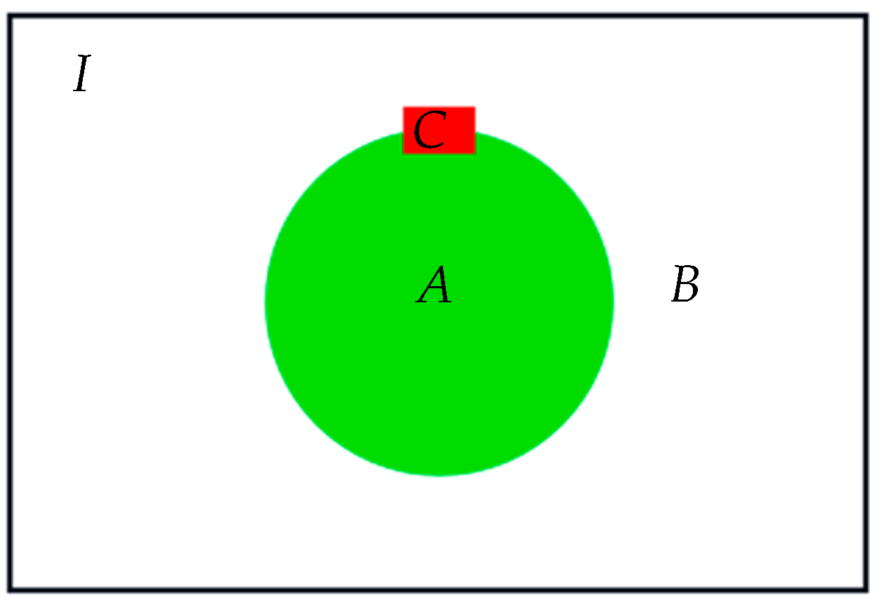
Suppose the specimen is described as a full set I and a defect inside the bulk of specimen is depicted by a subset A, such that the sound area (i.e., defect-free) inside I is the complementary set of A, which is called B. Obviously, A B = I . If any small segment of the defect edge is arbitrarily selected, the small local area surrounding the selected edge segment is called a sensitive region and it is depicted as C in Figure 2.
In this example, all image pixels of the thermogram (p) belong to two types of elements, that is, local defect pixels ( p A ) and local non-defective pixels ( p B ). When p A B , p is on the local defect boundary. Assume that the size of the sensitive region in this example varies from 10 × 10 pixels to 15 × 15 pixels such that it contains enough pixels to include two different types of pixels that are not too large or too small to define the defect boundary. In this example, all pixels inside the sensitive region are represented by ps. When the thermal wave front is diffused into the sensitive region, the temperature of ps is increased significantly due to the presence of the dislocation defect in the sensitive region. Since the sensitive region is slightly larger than the defect boundary, the statistics of ps, such as the standard deviation of all pixels in ps, is expected to vary in large magnitude when the thermal wave front is approaching (i.e., heating) and exiting (i.e., cooling) of the defect boundary.
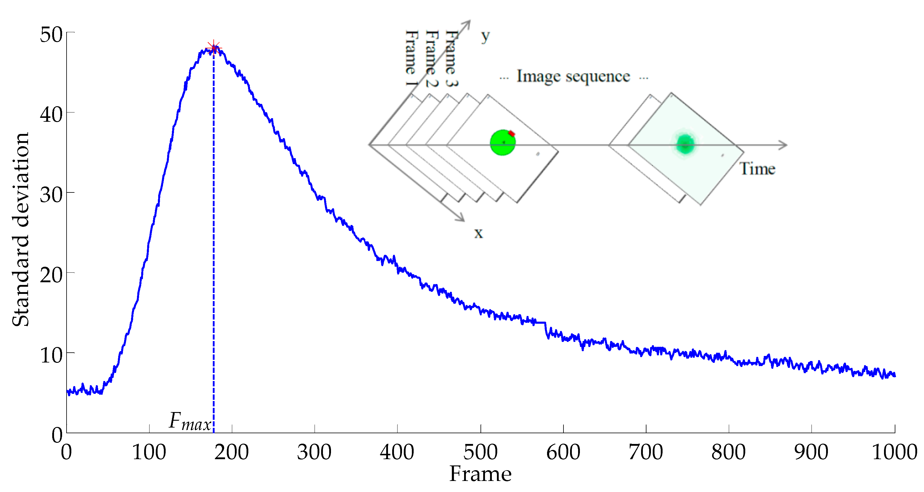
The insertion diagram in Figure 3 describes the process of recording the change of the surface temperature of the specimen in the form of sequence diagram. The curve of Figure 3 shows the standard deviation of the sensitive area as a function of the time, and the time can be replaced with a frame number. The peak of the standard deviation–time curve at Fmax depicts the maximum temperature differences between the defect and non-defect pixels. Therefore, the appropriate image frame can be abstracted for further image processing; thereby, the characteristics of the defect can be assessed accordingly. This methodology, which is known as the maximum of standard deviation of sensitive region method (MSDSRM), has been utilized for the automatic detection of defects in the specimen in this paper.

2.3. Automatic Defect Detection Framework (ADD)

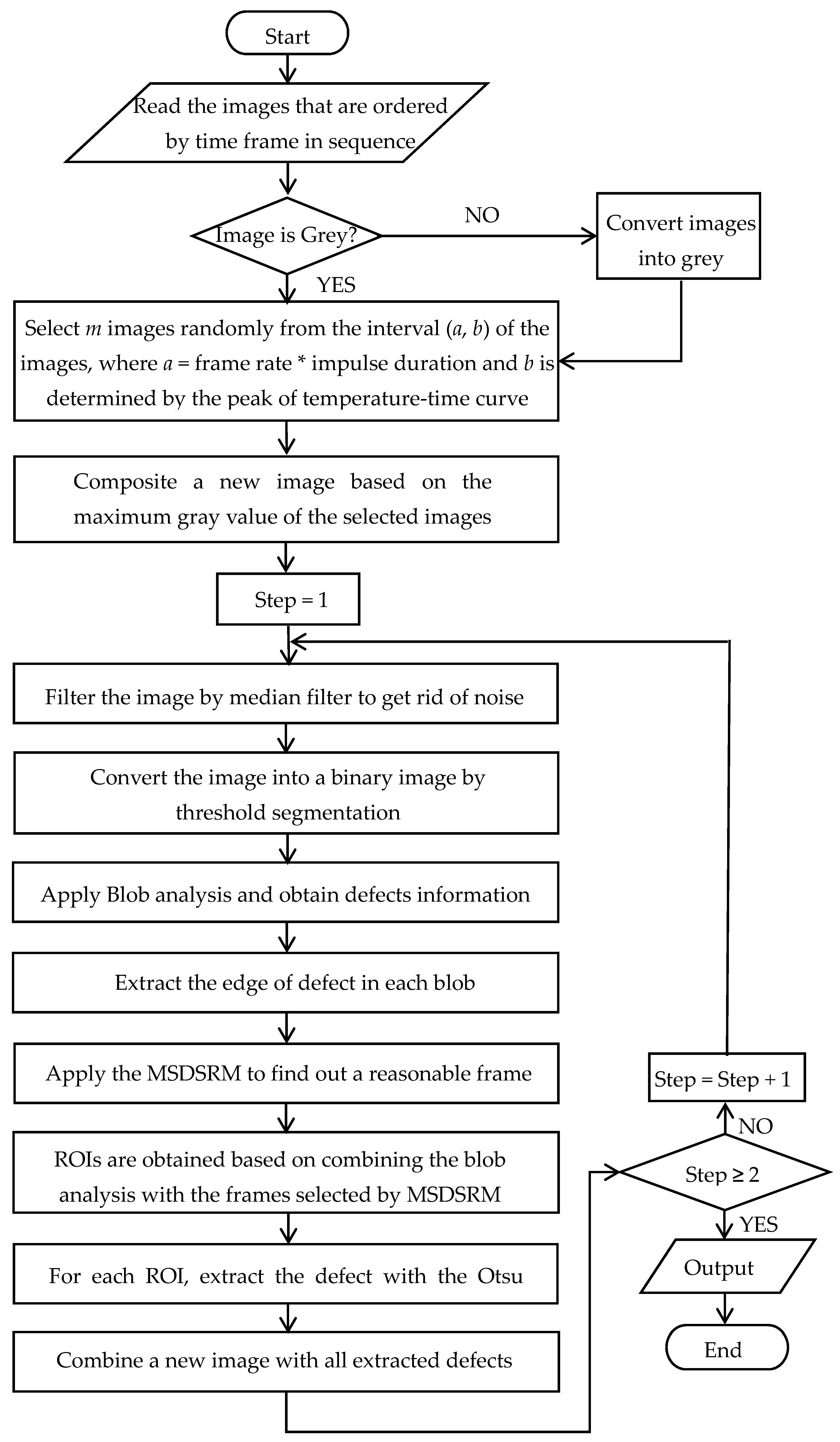
A two-step detection method for the automatic detection of defect (ADD) is depicted as a block diagram in Figure 4. A multi-image enhancement strategy is used to enhance the ability to detect deeper defects. The first step is the preliminary exploration of the defect, and on this basis, the second accurate detection is conducted to ensure the detection accuracy.
Note that there are two mechanisms that further guarantee the proposed ADD algorithm is fully automatic without the need of operator intervention for the selection of thermal frame image for processing, nor the need to determine the ROI (region of interest) dimension for defect diagnosis. Firstly, the MSDSRM selects suitable thermal frames for defect extraction, as described in this section. Secondly, the blob analysis has three functions as follows: (i) The blob analysis offers the basic information such as the defect distribution and the total number of defects; (ii) The edge of the defect in a blob can help locate the exact location of the sensitive areas. (iii) The blob analysis in conjunction with the MSDSRM allows the determination of the ROI for defect segmentation.

3. Material and Experiments

3.1. Material

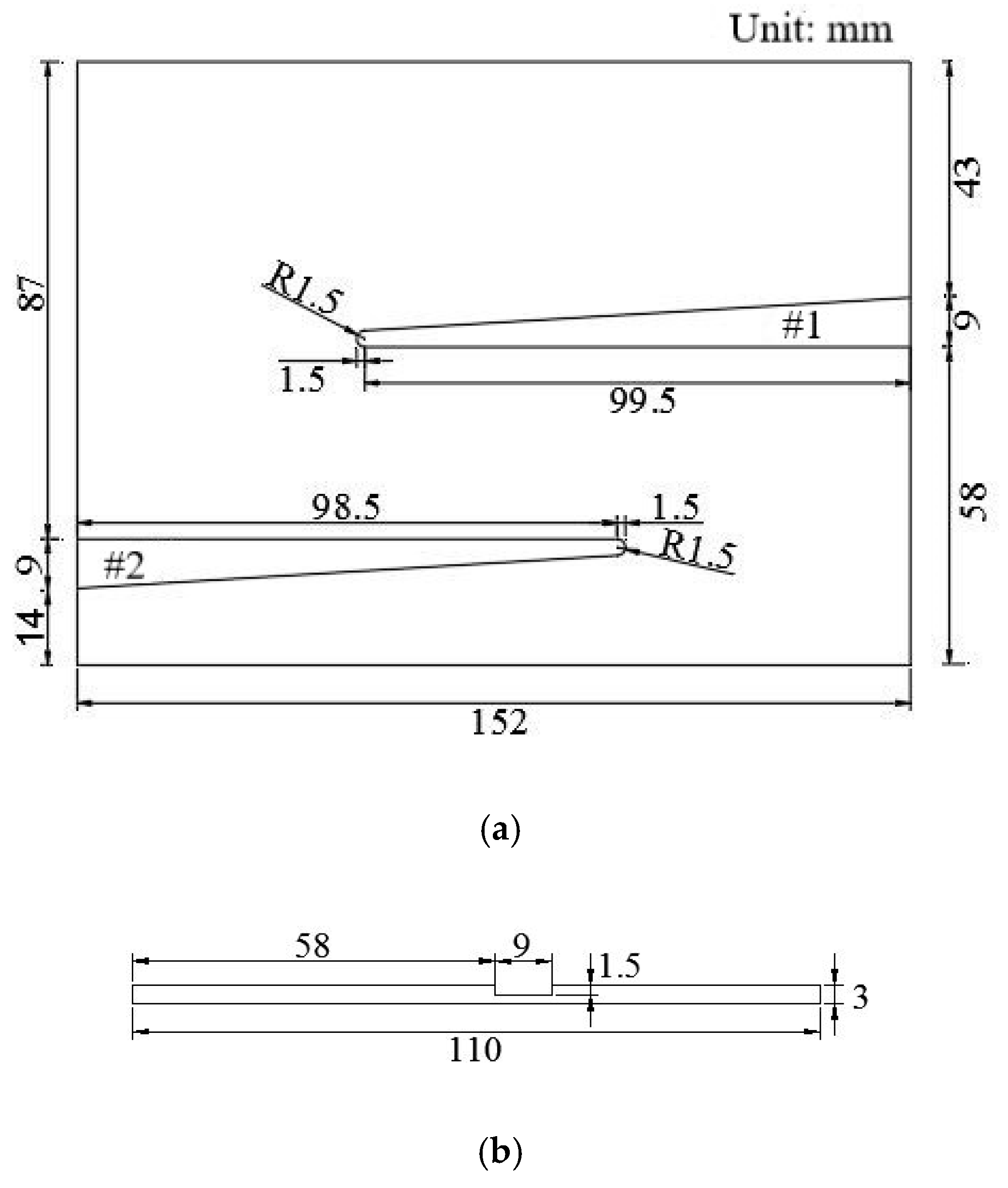
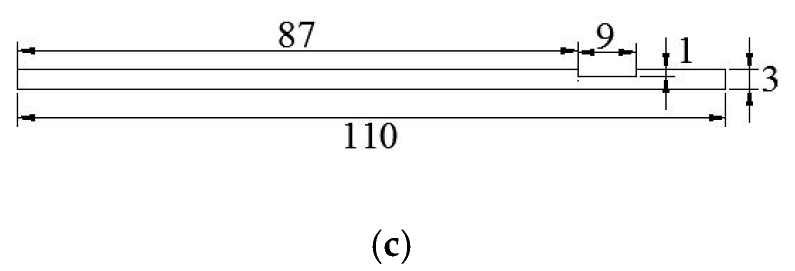
A PVC plate that has two flat-bottomed defects artificially fabricated at different depths is used as the main specimen in this paper (see Figure 5). The PVC has dimensions of 152 mm × 110 mm × 3 mm, and the two defects #1 and #2 have maximum width of 9 mm and 3 mm width at the narrow point with a semicircle tip with a diameter of 3.00 mm, as shown in Figure 6. The lengths of #1 and #2 grooves are 101 and 100 mm, respectively. The depths of #1 and #2 defects are 1.50 and 1.00 mm, respectively.

3.2. Experimental Setup: Long Pulse Thermography System

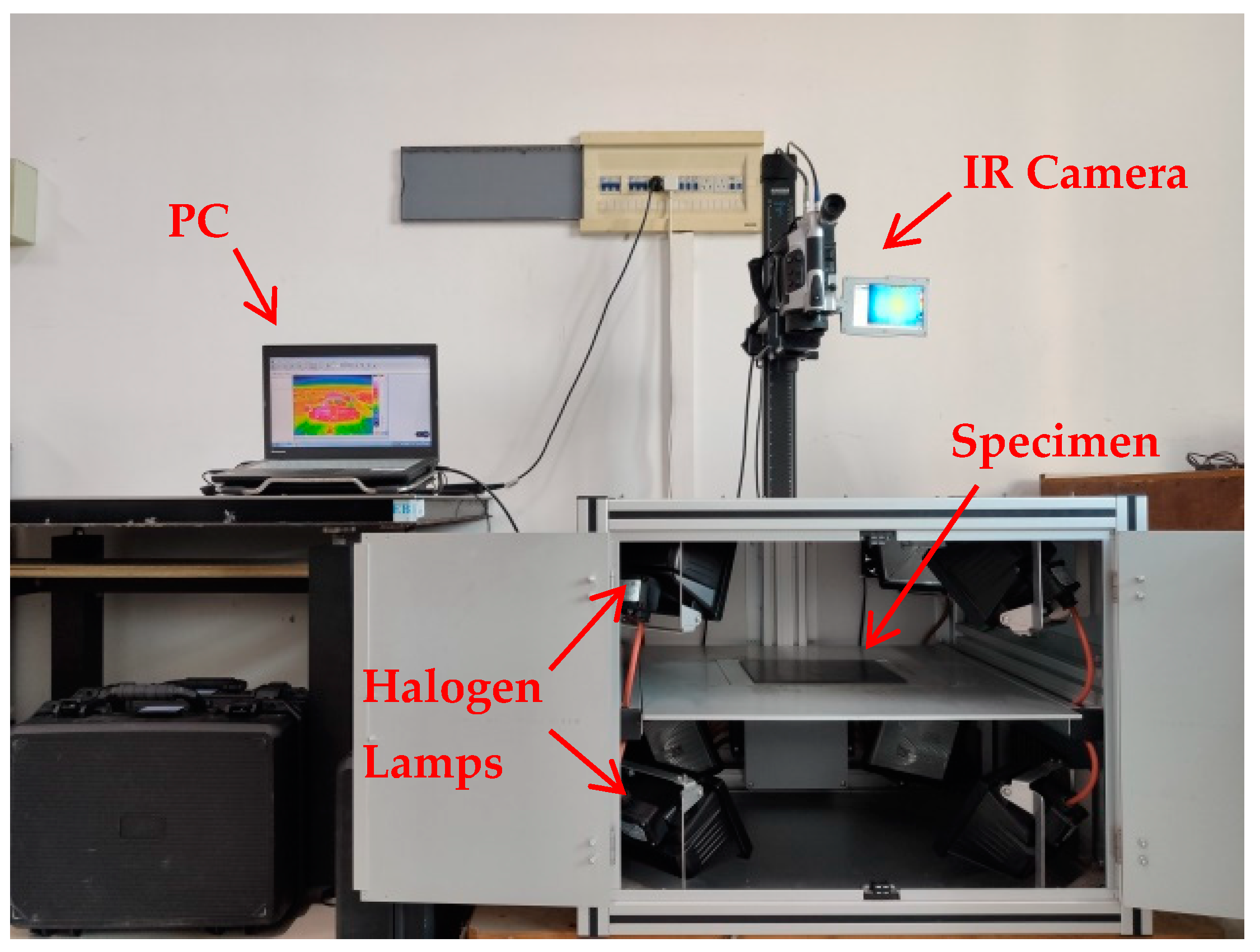
The synchronized infrared image acquisition system that has been employed in this work is schematically illustrated in Figure 7. The infrared imager in the system is an uncooled InfraTec VarioCAM® HD980 (made in Germany) with a detector resolution of 1024 × 768 and a maximum acquisition frequency of 30 Hz. The excitation source is composed of four 400 W halogen lamps. The controller controls the synchronization of excitation and acquisition. During the process of the experiment, the halogen lamps are triggered by software to generate pulsed radiations toward the test object. The infrared camera is simultaneously triggered to start recording as soon as the pulsed radiation is initiated.

3.3. Typical Thermogram

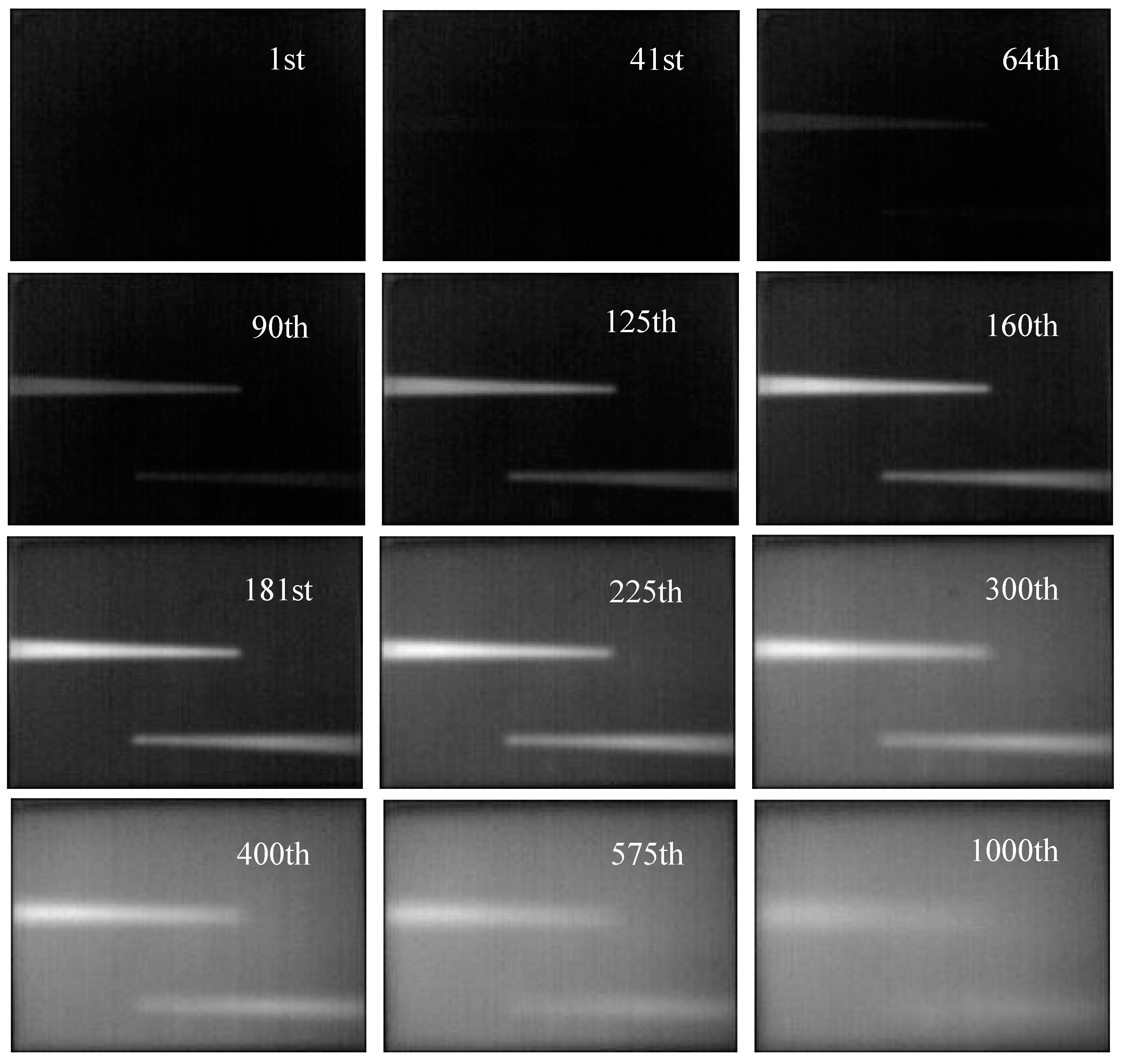
As shown in Figure 7, the infrared sequence was captured by a transmission mode, where excitation and an IR camera are located on the opposite side (the four halogen lamps in the bottom of the excitation box are used as the excitation sources). Figure 8 depicts samples of the 1000 frames of thermograms acquired at a frame rate of 30 Hz after a 3 s of heat pulse is irradiated toward the specimen, as described in Section 3.1. The heating and the cooling process can be seen vividly from Figure 8. It is seen that the thermal accumulation at the defects #1 and #2 began to appear at the 41st and 64th frames, respectively. Both defects can be seen clearly from the 125th to 225th frames, and their edges are subsequently seen to diffuse away at about the 575th frame.

4. Data Post-Processing

4.1. Image Composition and Its Image Processing

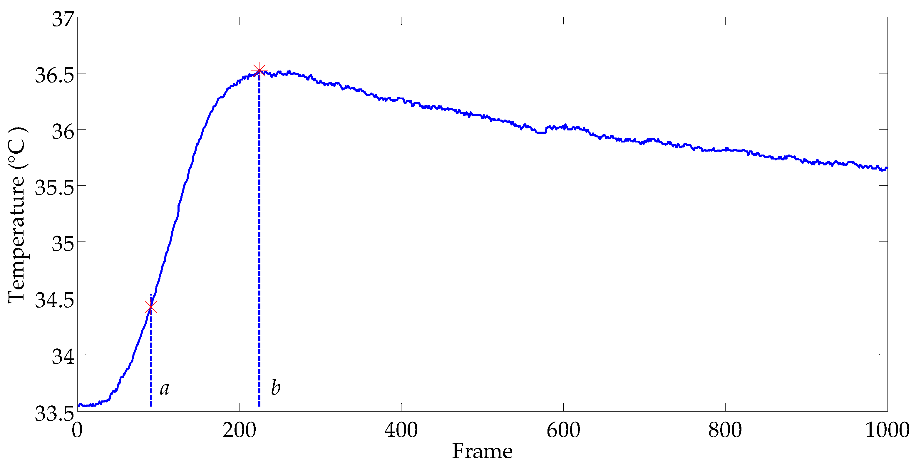
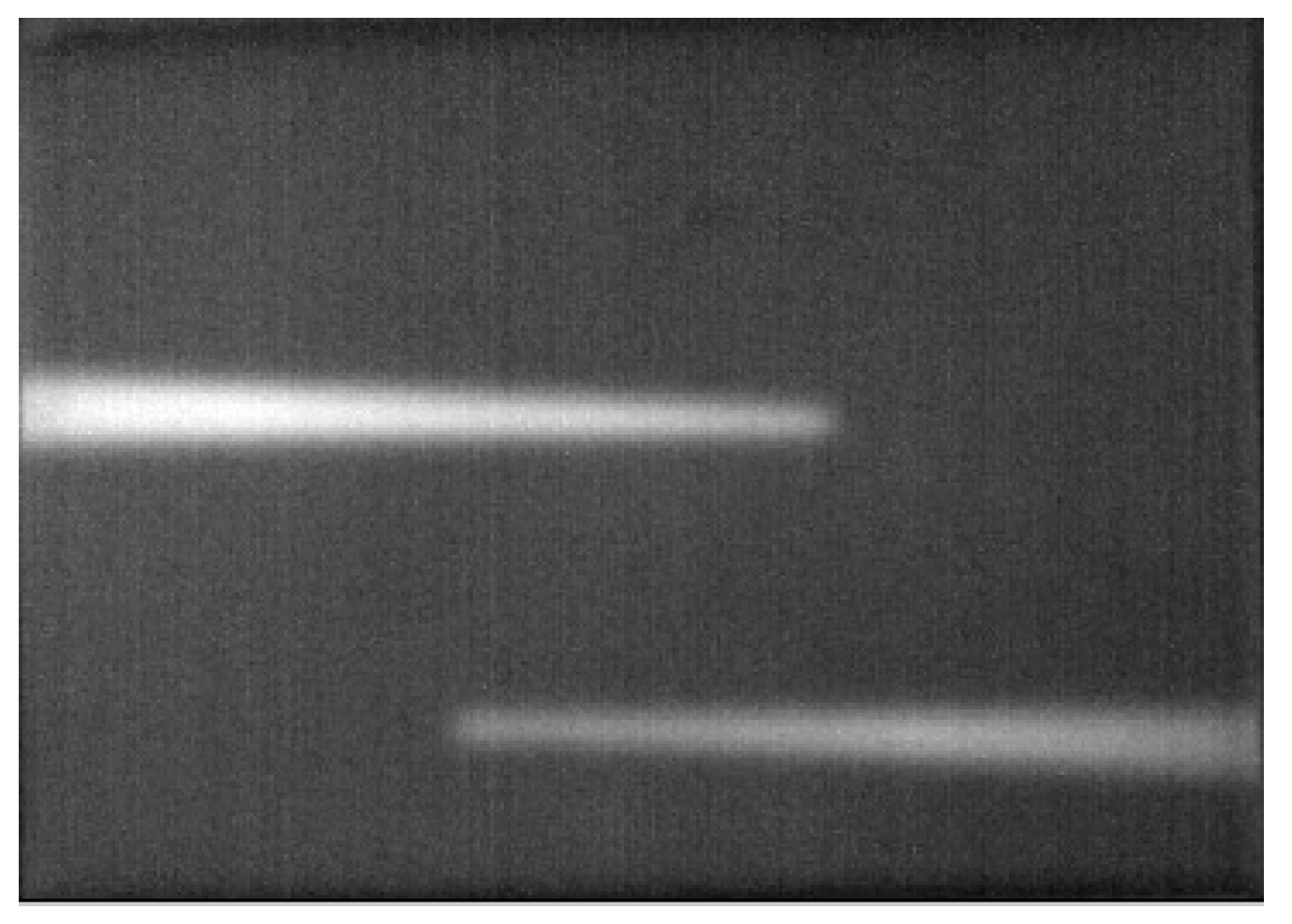
It can be seen from Figure 8 that not all frames from the obtained image sequence are suitable to carry out image processing for defect detection. The shallower defect appears earlier and brighter than the deeper one and has an advantage in the picture. To detect the deeper defect, a stratagem of image composition is proposed. Suppose that an infrared image sequence includes n images marked as I{i}, where i = 1, 2, 3 … n, and each image has a size of w × h. Select m images randomly from an interval (a, b) of the sequence, where 1 < a < b < n is marked as Ic{j} and j = 1, 2, 3 … m. The composition is based on the maximum gray value of the m images for each pixel. The composition image enhances the gray value of defects, especially the deeper one, and it can guarantee to detect all defects by image processing, as whole or partial. The values of a can be determined by the frame rate (f = 30 Hz) and impulse duration (t = 3 s); then, a = t * f = 90. The surface temperature of the shallower defect with time could be monitored by the infrared image sequence. There is a curve of temperature with time or frame in Figure 9. We can select the peak frame as the value of b. In this experiment, the value of b is 224. Therefore, the suitable frame range is (90, 224). We randomly select m frames from the interval (90, 224). If the deeper defect cannot be detected or the partially detected is too small, the value of m should be increased to be sure that a defect corresponds to a blob. We find that m = 10 provides enough feature information, and the composition result is shown in Figure 10.
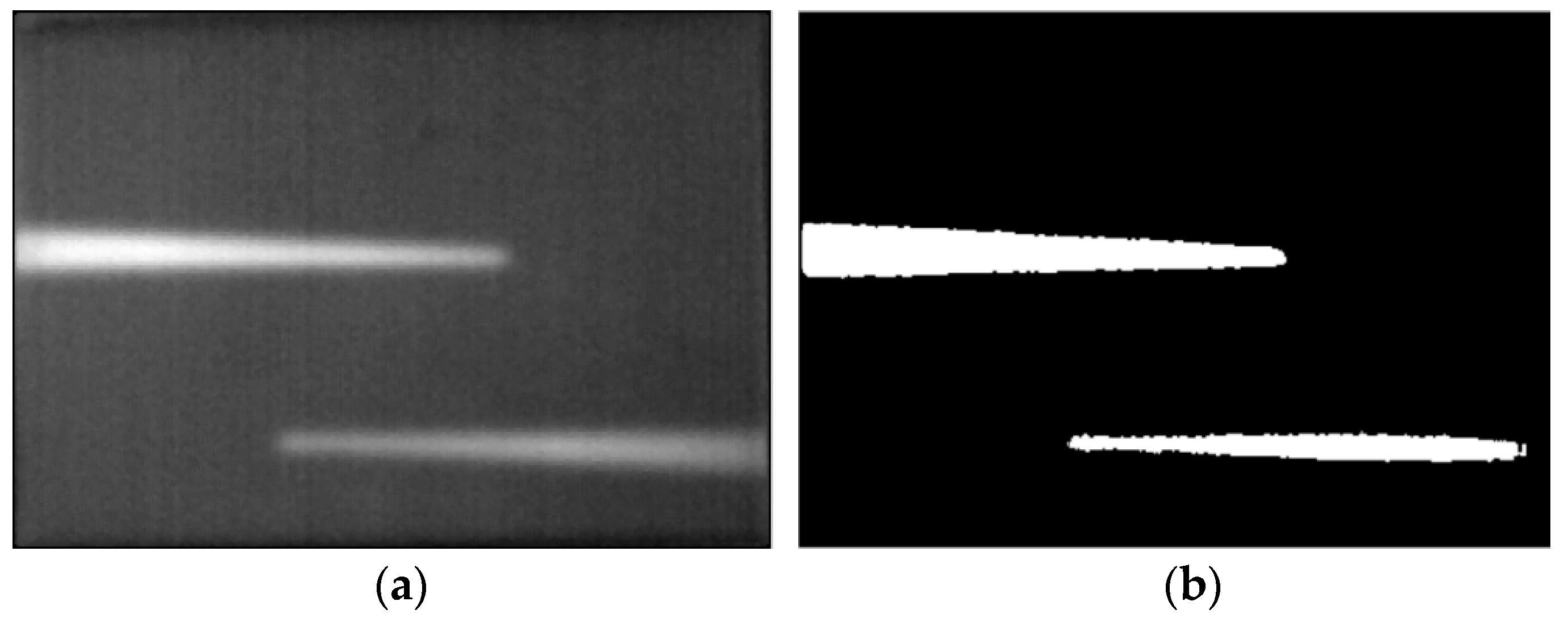
There are some factors, such as the non-uniformity of excitation and fringe effect of specimen, which may influence images detected by an infrared camera. The noise will affect the image composition. To reduce noise, a filter should be applied to the image composition. A 3-by-3 median filter is carried out to the image composition shown in Figure 10 and the result can be seen in Figure 11a. Then, the image is segmented by Otsu’s method as represented as Figure 11b.
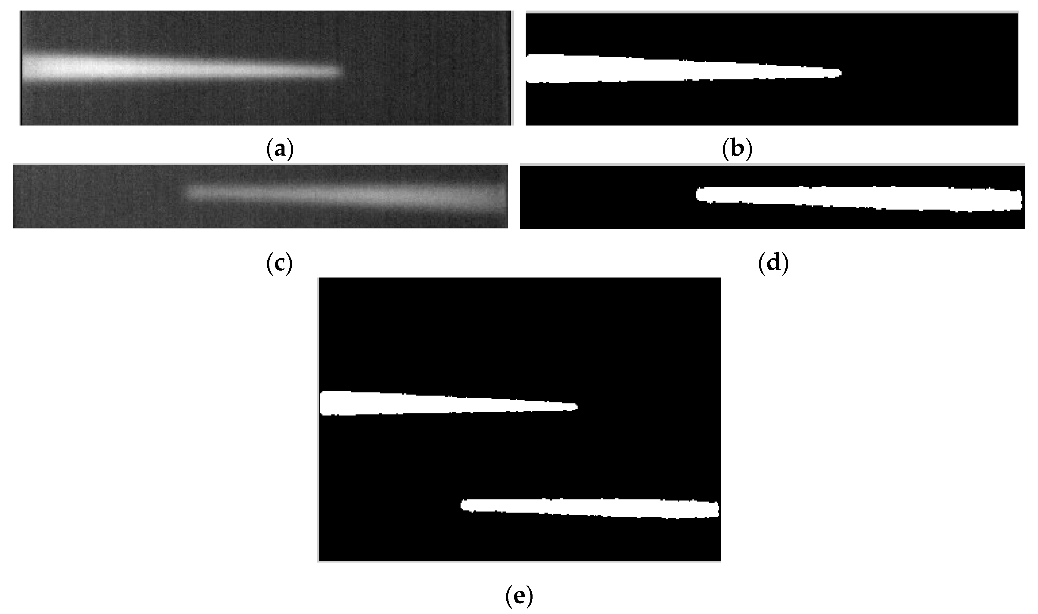
The extracted defect shape indicates that the obtained defect #1 is similar to the artificial defect, while the segmentation of defect #2 is obviously smaller than the real one and the root portion of the wedge groove has not been extracted, because defects #1 and #2 have different burial depths and their temperatures of heating to cooling process are out of sync. Under the excitation of 3 s optical pulses, defect #1 with shallow burial depth transferred heat more quickly to the surface of the specimen than defect #2 (with deeper burial depth), thus accumulating more heat on the surface. The higher temperature is reflected by the greater gray value in the corresponding area of the thermogram. The gray value of defect #1 plays a dominant role in the binary image segmentation of the entire image, leading to an incomplete extraction of defect #2. Even though defect #1 can be extracted completely with its shape similar to the real one, the relative error in area of the resulting defect is as high as 27.08% (see Table 1). This suggests that the value of binary threshold (0.47) of the full image by the Otsu method is not optimal for both defects. It is important to seek a ROI for every defect. We will discuss ROI determination in a later section.

4.2. Primary Detection of Defects

4.2.1. Blob Analysis

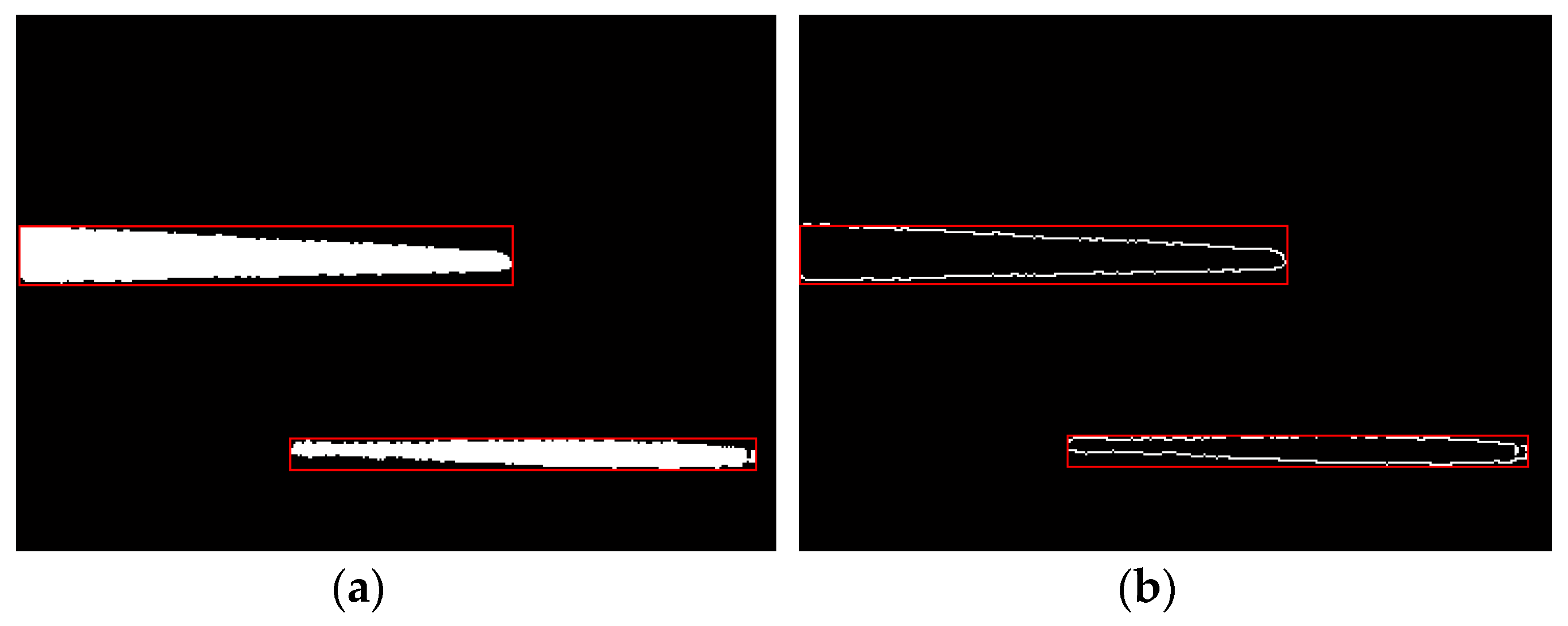
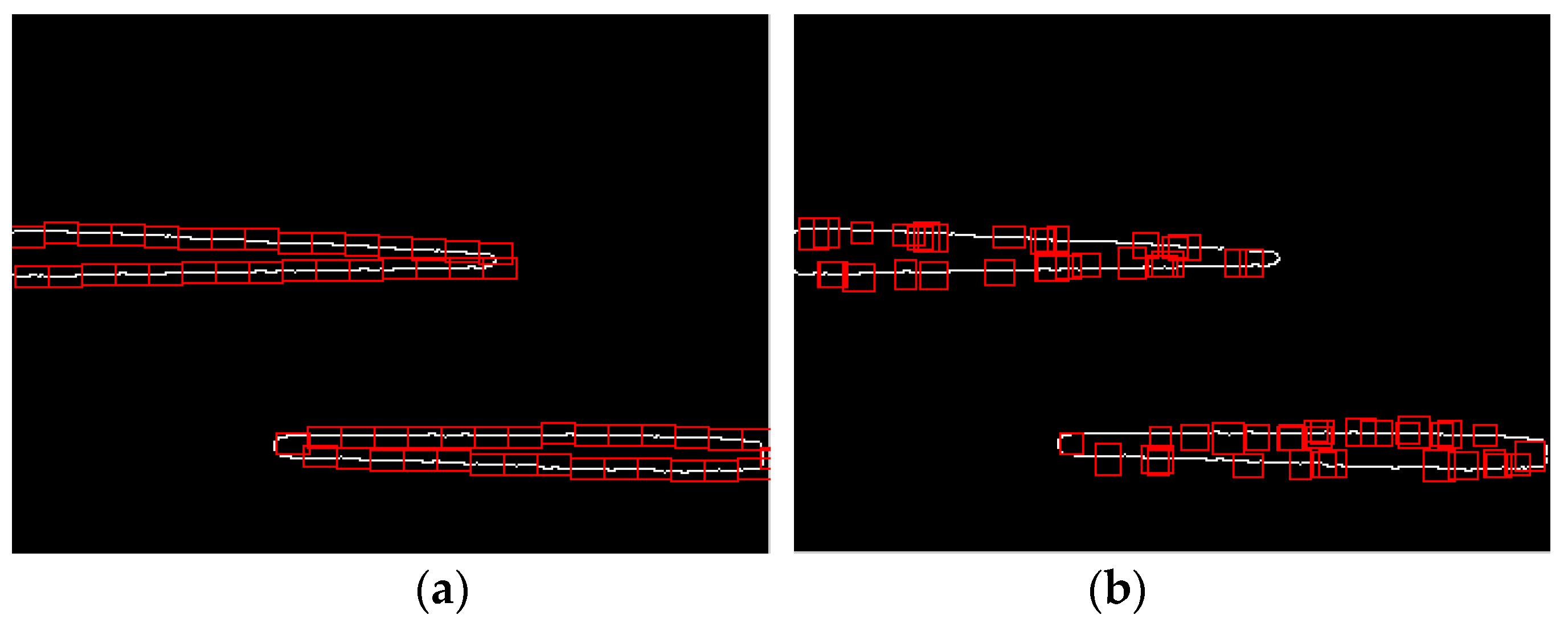
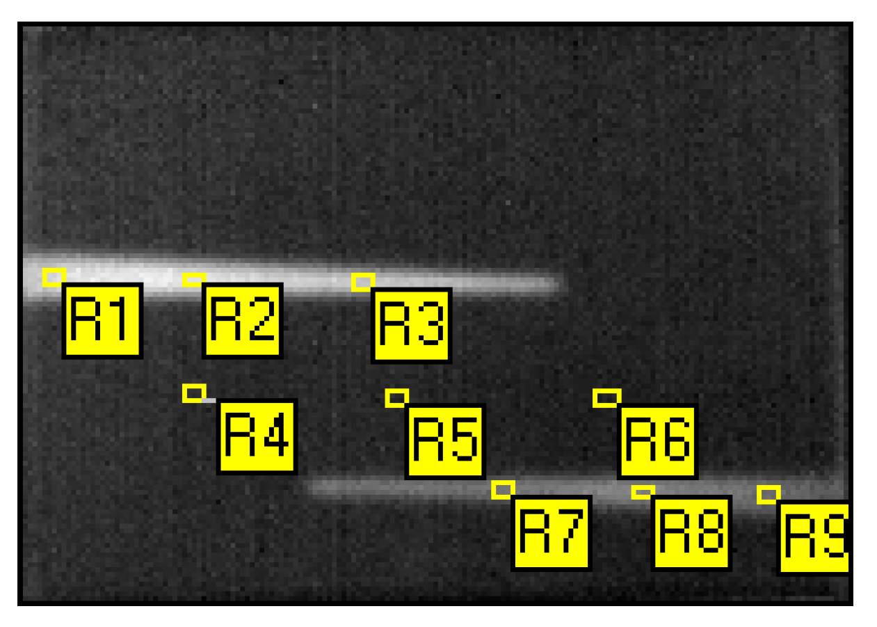
The blob analysis is used in the binary image, Figure 11b, by the blob analysis package in MATLAB. Defect regions are divided as blobs marked as red rectangles in Figure 12a. Features such as area (i.e., the number of pixels), center of gravity, or the orientation of a blob or blobs are calculated. Each blob contains one defect that is abstracted as a whole or portion (see the white line in Figure 12b). Moreover, a blob and a defect are one-to-one correspondence, so we can deal with blobs in turn equaling the process defects one by one. At last, the edges are abstracted by a canny operator for the further localization of the sensitive region.

4.2.2. Frame Determined by MSDSRM

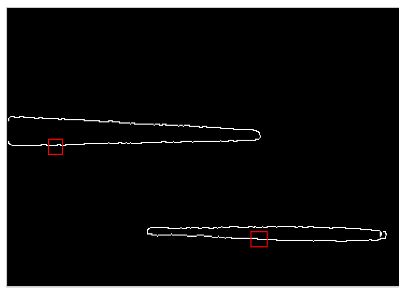
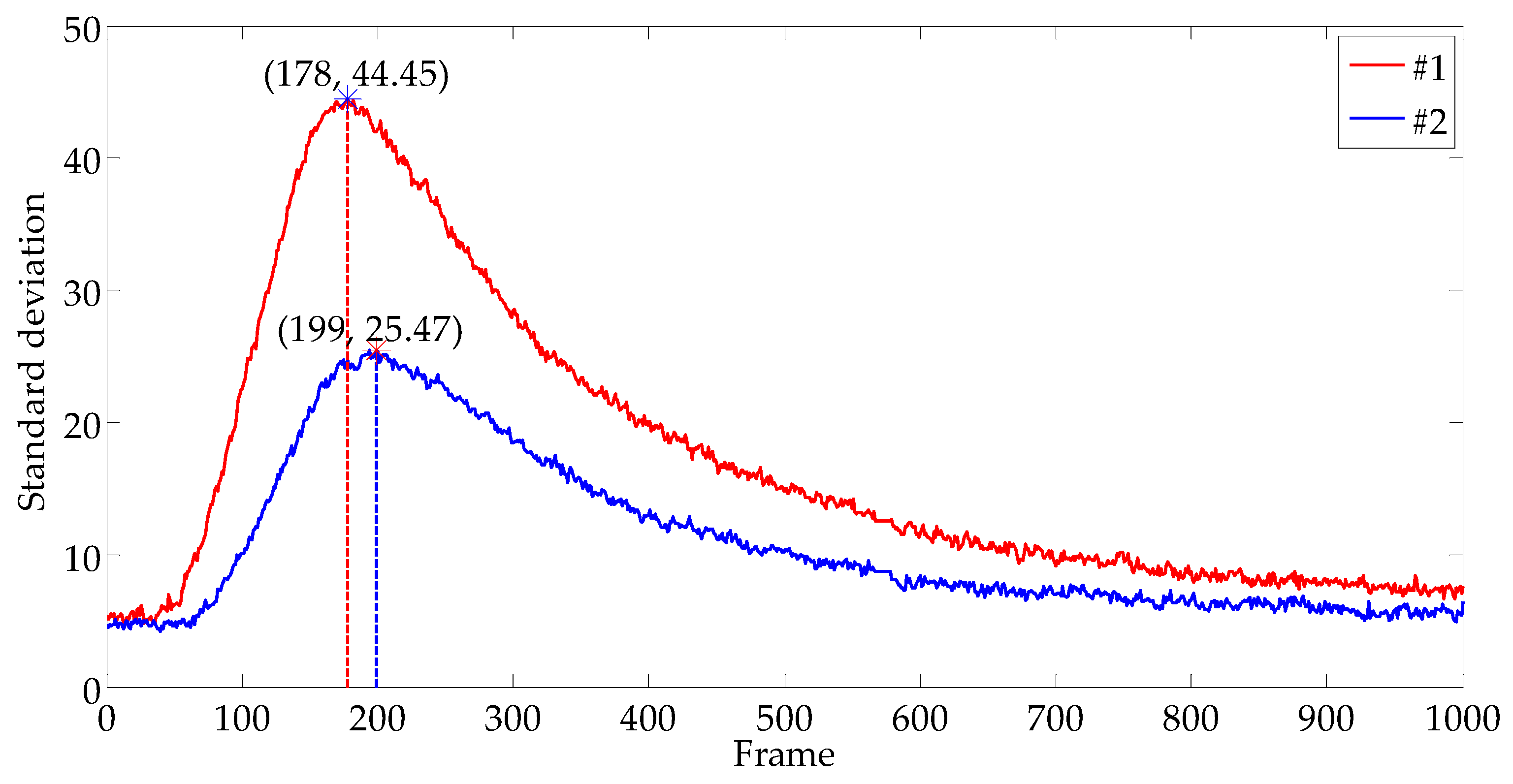
For each segmented defect region, the proposed MSDSRM is used to determine a suitable frame to calculate the defect boundary. A sensitive region, as shown in Figure 13, is randomly located based on the edge of the detected defect, and its size is also randomly selected from a range in (10, 15) × (10, 15) as mentioned above. Through monitoring the history of standard deviation of the sensitive region with time in the infrared image sequence, we can get the curve of standard deviation of the sensitive region vs. time as shown in Figure 14. It shows the standard deviations for the two defect regions for the whole set of the infrared image sequence (1000 frames). Defect #1 reaches its peak standard deviation of 44.45 at Frame 178, while defect #2 reaches its peak standard deviation 25.47 at Frame 199. Therefore, we consider that Frame 178 is reasonable for extracting defect #1 and Frame 199 is reasonable for extracting #2.

4.2.3. Determination of ROI and Extraction of Defects

ROI centers its corresponding blob and expands around it. For example, the blob is expanded twice its size in four directions i.e., up, down, left, and right, respectively. At the same time, ROI is restrained by the specimen boundary and its neighbor blobs.
Figure 15 is a sketch of ROI based on blob and restrained by constraints, where the yellow area is a blob, and it expands the blue rectangle, but the red dotted portion is ROI due to the specimen boundary and neighbor blobs.
The ROIs for each defect are determined as shown in Figure 16a,c, which are selected by the MSDSRM. After a median filter, defects #1 and #2 are respectively extracted by automatic threshold segmentation with the value of 4.6 and 3.6 determined by the Otsu method, as shown in Figure 16b,d. The relative errors are 2.08% and 2.91% for defects #1 and #2 respectively, as seen in Table 2. The value of threshold is important in image segmentations, which can influence the integrality and veracity of the results. The Otsu method based on the maximum of between-cluster variance is always considered an optimal method of thresholds for automatic selection. It will divide the processing image into two categories, i.e., background and objectives. The optimal threshold is obtained by searching the maximum between-cluster variance. Comparing the data in Table 1 and Table 2, the threshold changes very little from 0.47 to 0.46 for #1 and to 0.36 for #2, but the error of defect #1 decreases from 27.08% to 2.08%, and the error of defect #2 reduces to 2.91%, which is incomplete extraction after processing the full image, as shown in Figure 11b. At last, the two segmentation images are combined as a whole (see Figure 16e). The semicircular arc of the defect tip can be extracted accurately.

4.2.4. Performance Analysis of Primary Detection Results

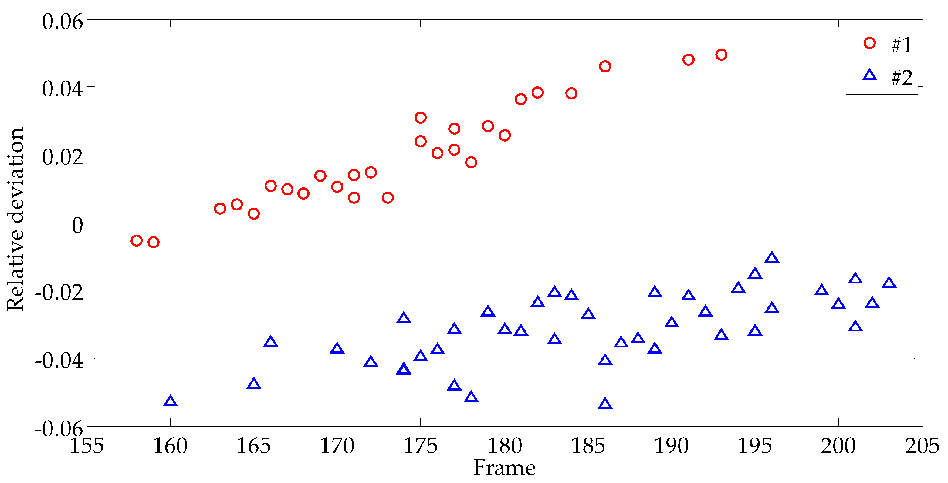
To assess the performance of primary detection results, 100 independent experiments were conducted to extract each defect. Each composition image was synthesized by 10 random frames from the interval (90, 224) of the infrared sequence, and the location and size of the sensitive regions in each experiment were randomly selected, too. Figure 17 shows the discrete distribution map of the deviation of the extracted defect area from the ground truth. The symbols “Ο” and “Δ” in the figure represent defects #1 and #2, respectively. From the figure, we can see that the frame selected by MSDSRM ranges within (155, 205) less than 50 frames. We have obtained a very narrow range from the original image sequence of 1000 frames, so it is a good primary detection. Defect #1 is the shallow defect, and there is a tendency that the relative error gradually increases with time. However, there is no regularity for #2. Moreover, there are serious overlaps of frames for different defects at different depths. There are two reasons for this phenomenon: one is that the edge extracted from the composite image is not the exact boundary of the defect, especially for the deep one shown as Figure 11b, which is smaller than the true; the other is that single sensitive region chosen randomly is not always representative of the whole standard deviation around the defect due to the non-uniformity of excitation. Under the same excitation, the heat transmission speed in the defect area varies with the burial depth. For the defect with a shallow burial depth, the corresponding surface temperature rises faster, taking less time to form a temperature difference area coinciding with the defect shape. In contrast, the defect with a deeper burial depth takes more time to form a temperature difference area coinciding with the defect shape. The best image for processing defect #1 should be a frame in sequence ahead of that for processing defect #2. So, the results of primary detection should be improved further to maintain the results’ robustness.

4.3. Secondary Detection of Defects

4.3.1. Improvement of Detection Results

The sensitive region for further detection can be selected from the edge of the detected defect base on the primary detection of defect edge as seen in Figure 16e. To alleviate the effect of heating inhomogeneity of the specimen, the average value of standard deviation of multiple sensitive areas is calculated instead of the single one. Two sensitive region selection methods are discussed:
(i)
Uniform selection (Figure 18a): sensitive regions are followed one by one along the edge of the defect. The total number of sensitive regions is determined by the perimeter of the defect extracted at the primary detection. The size of the sensitive region is set to 10 × 15 pixels.
(ii)
Random selection (Figure 18b): thirty sensitive areas are randomly selected from the edge of the defect. The size of the sensitive region is randomly decided within the range of (10, 15) × (10, 15) pixels.
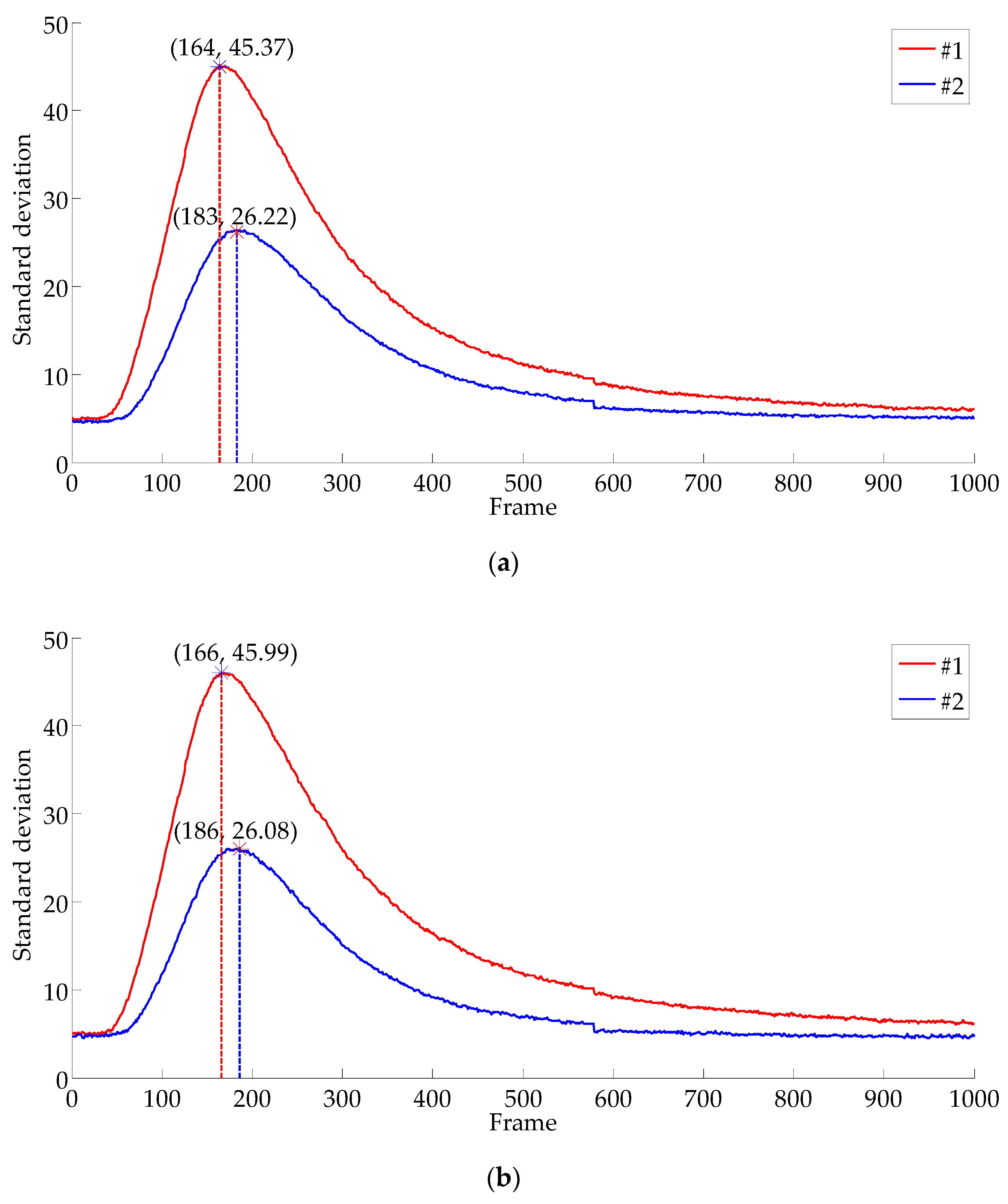
Figure 19 shows the standard deviations for the two defect regions for the whole set of the infrared image sequence (1000 frames). The results yield smother curves than the traditional measurement (see Figure 14), and the peak value of a given curve becomes easier to identify. For example, for uniform selection (Figure 19a), defect #1 reaches its peak standard deviation 45.37 at Frame 164, while defect #2 reaches its peak standard deviation 26.22 at Frame 183; for random selection (Figure 19b), defect #1 reaches its peak standard deviation 45.99 at Frame 166, while defect #2 reaches its peak standard deviation 26.08 at Frame 186.
It can be seen that for each defect, two methods produce similar results, which suggests both methods work well. However, such results differ a lot with the two defects because the two defects have different depths. The peak standard deviation indicates that the defect and non-defect areas have reached the maximum degree of differentiation in that frame. As a result, that frame should be selected to extract the defect boundary. Therefore, we consider that Frame 164 is reasonable for calculating defect #1 and Frame 183 is reasonable for calculating #2, by uniform selection of sensitive regions, while Frame 166 is suitable for defect #1 and Frame 186 is suitable for defect #2 by random selection. The secondary detection results are shown as statistics in Table 3, which improve the result of primary detection (Table 2).

4.3.2. Analysis of Robustness

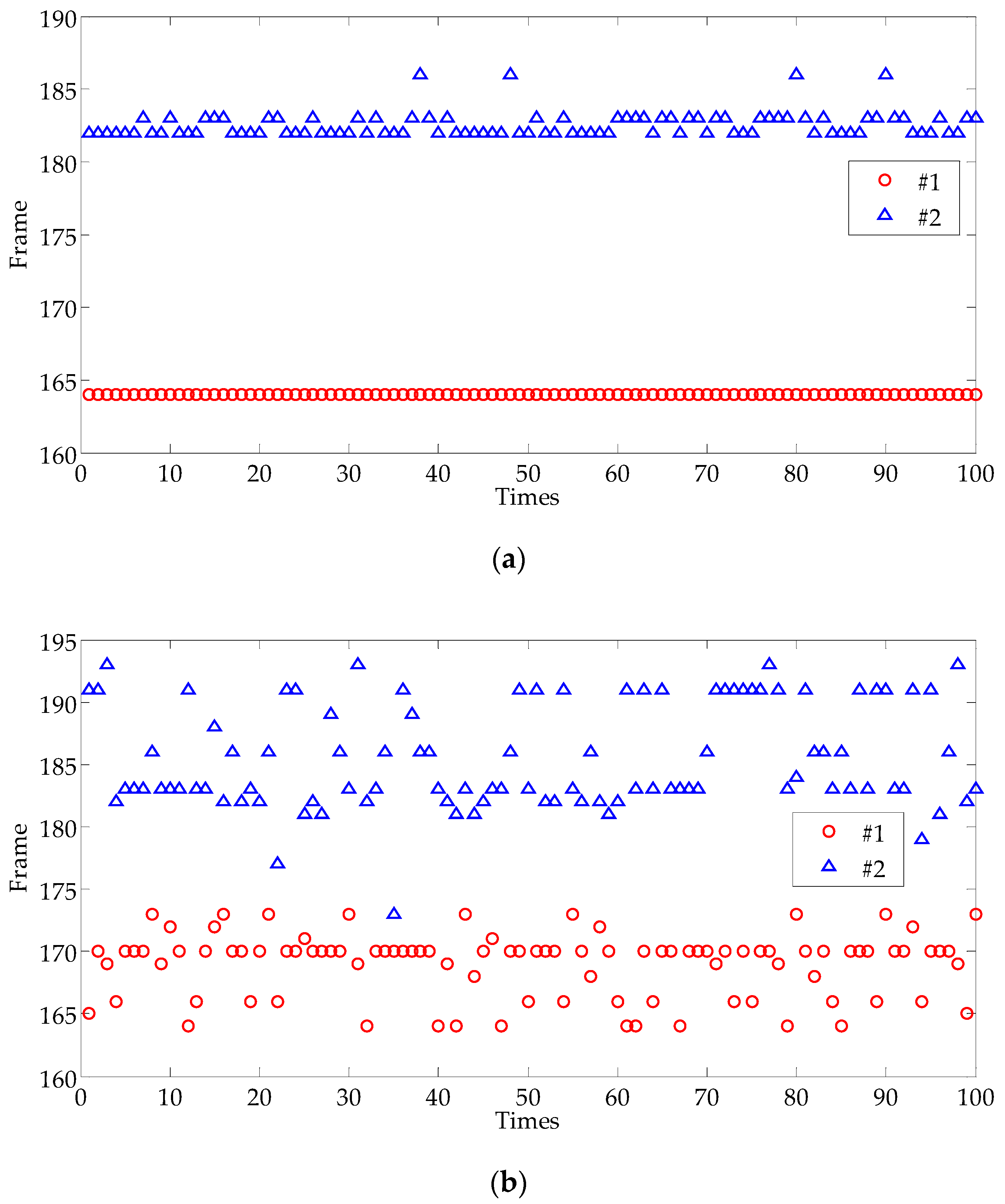
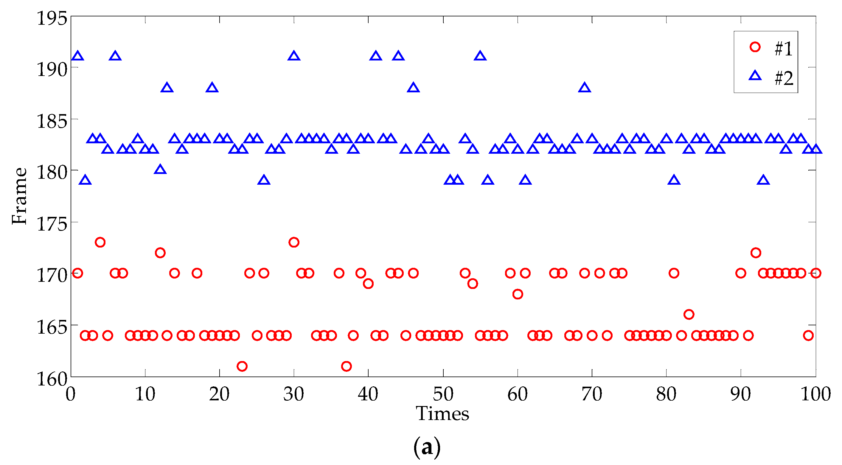
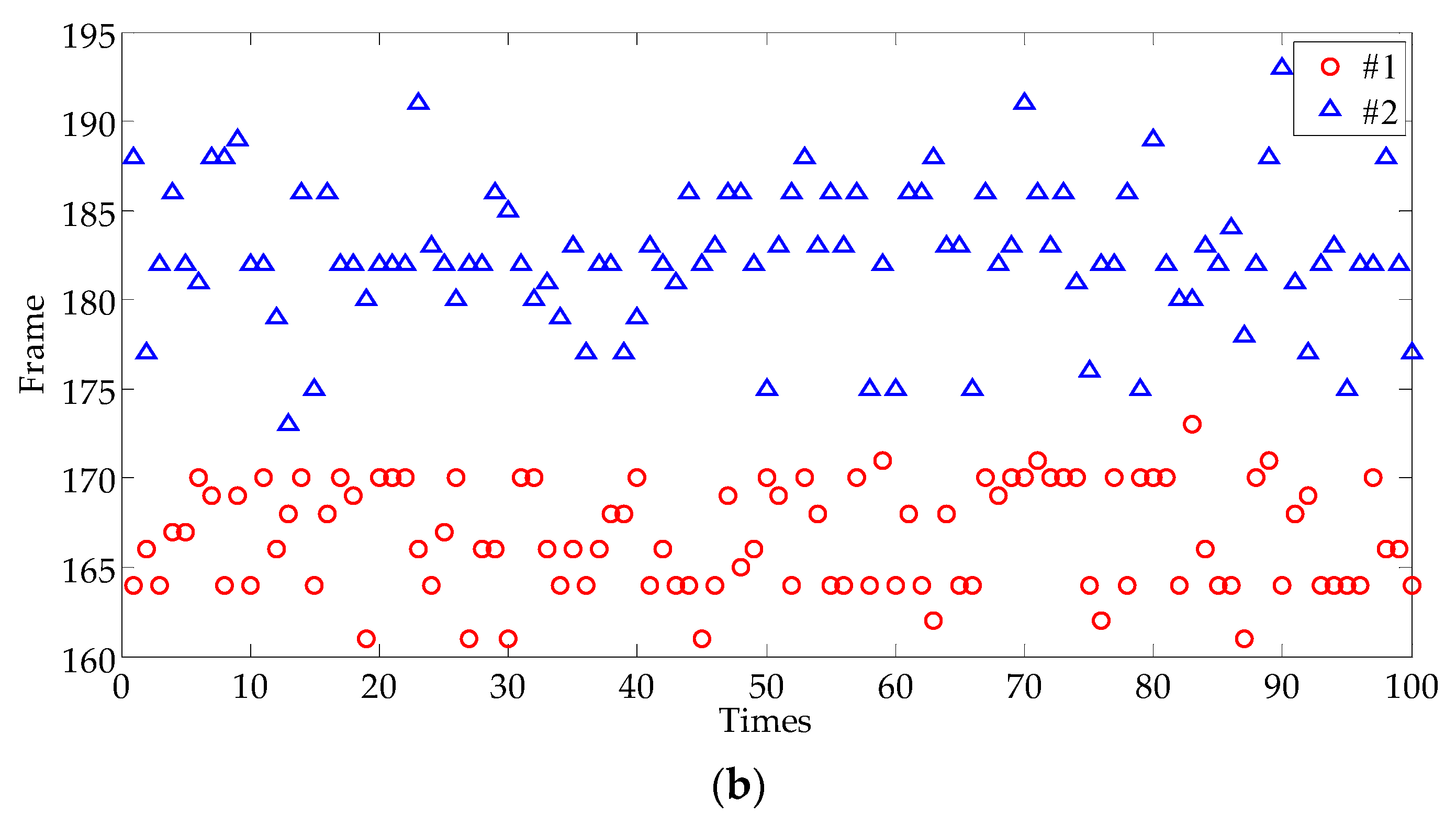
To assess the stability and reliability of the proposed automatic method, 100 independent experiments were performed. The results are shown in the scatter diagram Figure 20a,b by uniform selection and random selection, respectively. From Figure 20a, we can see that Frame 164 has a relative frequency of 100% to extract defect #1, and Frame 182 (56%), Frame 183 (40%), and Frame 186 (4%) are chosen for defect #2 using uniform selection. Figure 20b shows that using random selection, the suitable frames for #1 and # 2 are (164, 173) and (173, 193), respectively. The frames from the random selection scheme are more fluctuated than those from the uniform selection scheme, as expected. In either case, the frame selected for extracting defect #1 is ahead of those selected for extracting defect #2. This situation is consistent with Equation (7).
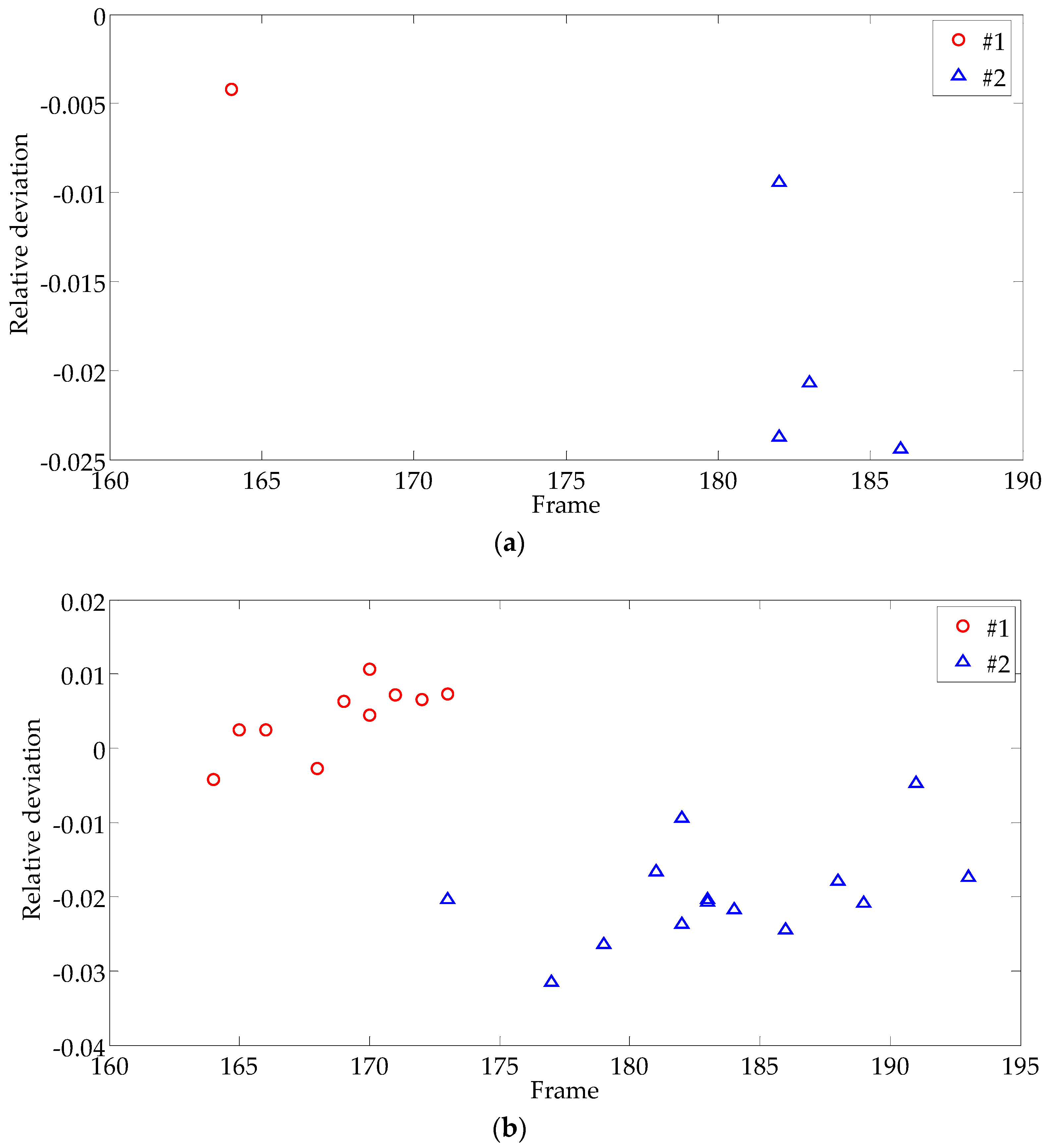
Figure 21 shows the discrete distribution map of the relative deviation of the extracted defect area from the actual size. The symbols “O” and “∆” in Figure 21 represent defects #1 and #2, respectively. By uniform selection, defect #1 can be accurately detected with 0.42% relative error and the error of #2 is within 2.5%, as shown in Figure 21a. From Figure 21b, the errors of defect #1 are all within 1.1% and those of #2 are within 3.2%. All in all, the MSDSRM with multiple sensitive regions is very useful for selecting an appropriate thermogram for extracting defects at different depths.

5. Discussion and Analysis

5.1. Influence of Size of Sensitive Region on Detection Results

To obtain a suitable frame from the sequence, the sensitive regions play an important role because the frame image is selected by the peak of the curve of the standard deviation of the sensitive regions vs. frames. We choose the shape of the sensitive region as a rectangle. Suppose the size is w × h, where w is the width of the rectangle and h is the height of the rectangle, respectively. The width is along to the detected edge of the defect, while the height is perpendicular to the local edge. Note that the detected edge might not be the exact true edge, such as the edge detected for defect #2 at the bottom of Figure 13, which is very different from the actual boundary. The influence of the size of the sensitive region on detection results in the primary detection and secondary detection phases are further investigated below.

5.1.1. Influence of Size of Sensitive Region in the Primary Detection

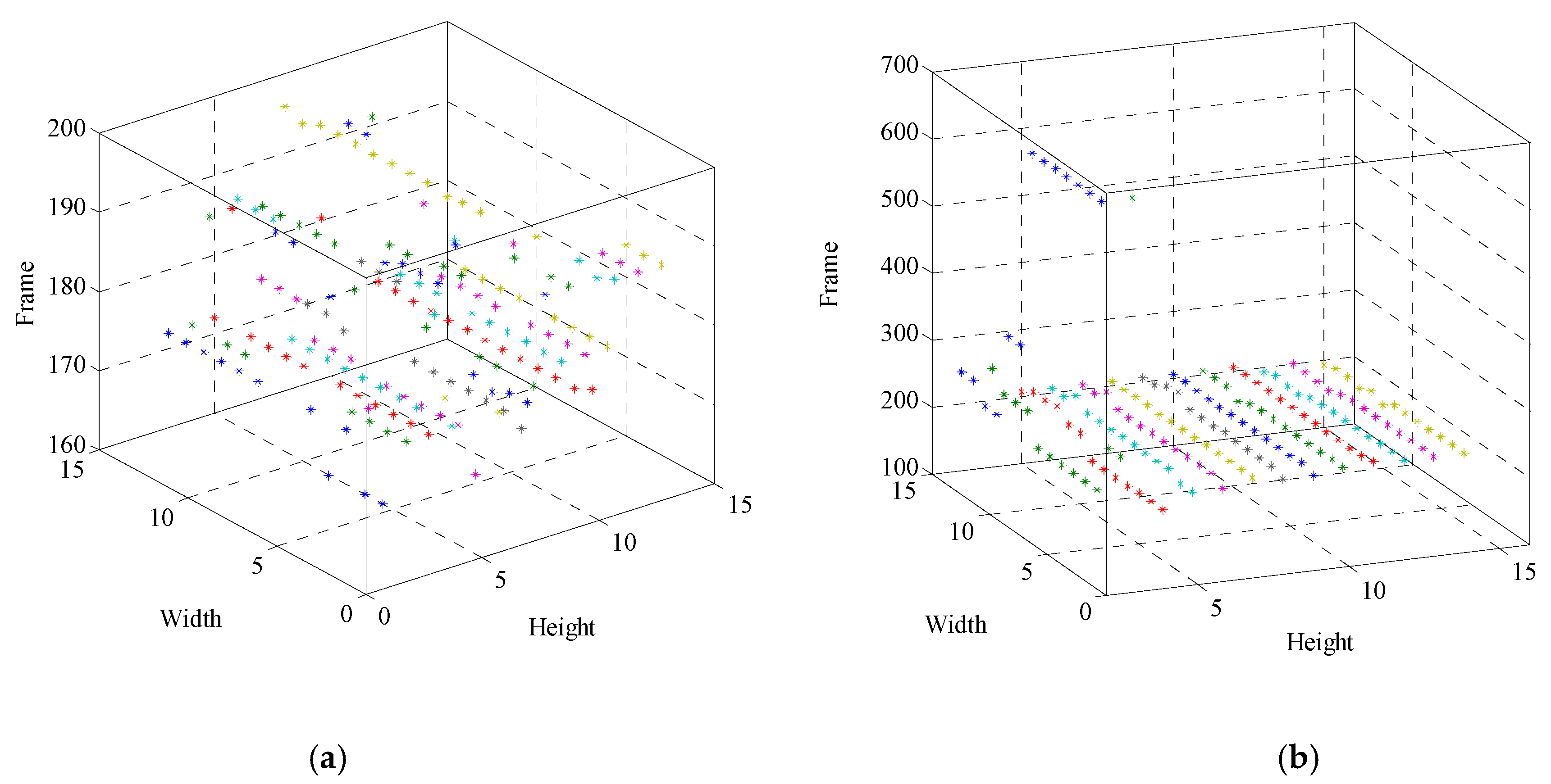
The setup of a single sensitive region during the primary detection is shown in Figure 13. We adopt a random method to locate a point on the extracted edge; then, we fix the point and sample the sensitive region size from 3 × 3 pixels, generally expending to 15 × 15 pixels around the point. That is, both the width and the height are changed from 3 pixels to 15 pixels. The step size change in both the width and height is 1 pixel, so there are 169 test areas in total.
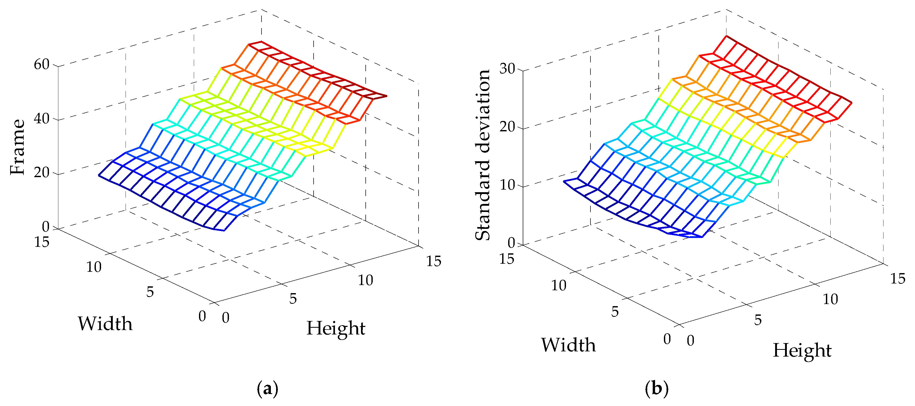
The standard deviations are calculated for every sensitive region in each image in the sequence, and the time history curves of standard deviation are obtained similar to the curves in Figure 14 and Figure 19. All peaks of the curve are collected to obtain the maximum standard deviation surface of different defects related to the sensitive regions with different widths and heights, as shown in Figure 22. Figure 22a,b are the surfaces corresponding to defect #1 and #2, respectively, and they have same shapes except that the values of standard deviation in Figure 22a are larger than those in Figure 22b. From these two figures, it can be seen that the values of standard deviation varying with height are larger than with width. It shows that the sensitive region change in height is more sensitive than in width, i.e., the direction of perpendicular to edges is much more sensitive than along the edges.
Due to each maximum of standard deviation corresponding to a frame, the selected frames are shown in Figure 23a,b for defect #1 and defect #2, respectively. For defect #1, all the selected frames are in the interval of (165, 196), which are similar to the results shown in Figure 17 and can be used as a suitable frame to carry out the primary detection. However, not all of the selected frames are suitable for defect extraction, and 5.92% of the results (10 data) should be eliminated because defects cannot be fully displayed. Frame 347 and Frame 646 in the middle and late stage of thermal diffusion are frequently chosen when the height of the size of the sensitive region is the minimum of 3. As mentioned before, the gray value of defect #1 plays a dominant role in the binary image segmentation of the entire image, leading to a complete extraction of defect #1 but incomplete extraction of defect #2. The results show that the higher the precision of defect boundary extraction, the less affected by the size of the sensitive area.

5.1.2. Influence of Size of Sensitive Region in the Secondary Detection

From the above discussion, all the sizes of the sensitive region from 3 × 3 pixels to 15 × 15 pixels can be sampled to seek a suitable frame in the secondary detection when a relative correct result is acquired in the primary detection. To discuss the influence of size of the sensitive region in the secondary detection, 100 independent experiments were done as in the previous section.
For uniform sampling, the size of each sensitive area sampling is the same, but the size is no longer fixed as the front. Instead, the size is randomly determined from 3 × 3 pixels to 15 × 15 pixels in 100 experiments. The results are shown in the scatter diagram shown in Figure 24a. Compared with the results of Figure 20a obtained by a fixed size of 15 × 10, it can be seen that the diversity of results is greater than that of previous results. Especially for defect #1, it is no longer only one value for Frame 164, and more frames are selected in the interval (161, 173). Among the results, Frame 164 and Frame 170 are chosen with large probability.
For random sampling, the parameters were set as the previous section except that the size of sensitive region variation range is enlarged from 3 × 3 pixels to 15 × 15 pixels instead of from 10 × 10 pixels to 15 × 15 pixels, and the results are shown in Figure 24b. Compared with the previous results (see Figure 20a), the range of frames found in the two statistical experiments was similar, except that defect #1 was slightly larger. This indicates that size has little influence on random sampling.

5.2. Compare with Other Frame Selection Methods

5.2.1. Maximum Temperature Difference Method

In many cases of defect detection, the image with the largest temperature contrast is used, i.e., the image where the temperature difference between the defective area and the sound surface is the largest [4]. To have an accurate defect size, there is a need to analyze the specific IR image captured at tmax (time that records ΔTmax) or immediately after it [5], and the method is called the maximum temperature difference method (MTDM), which give a method of how to determine a key frame from the image sequence as an original image to image processing.
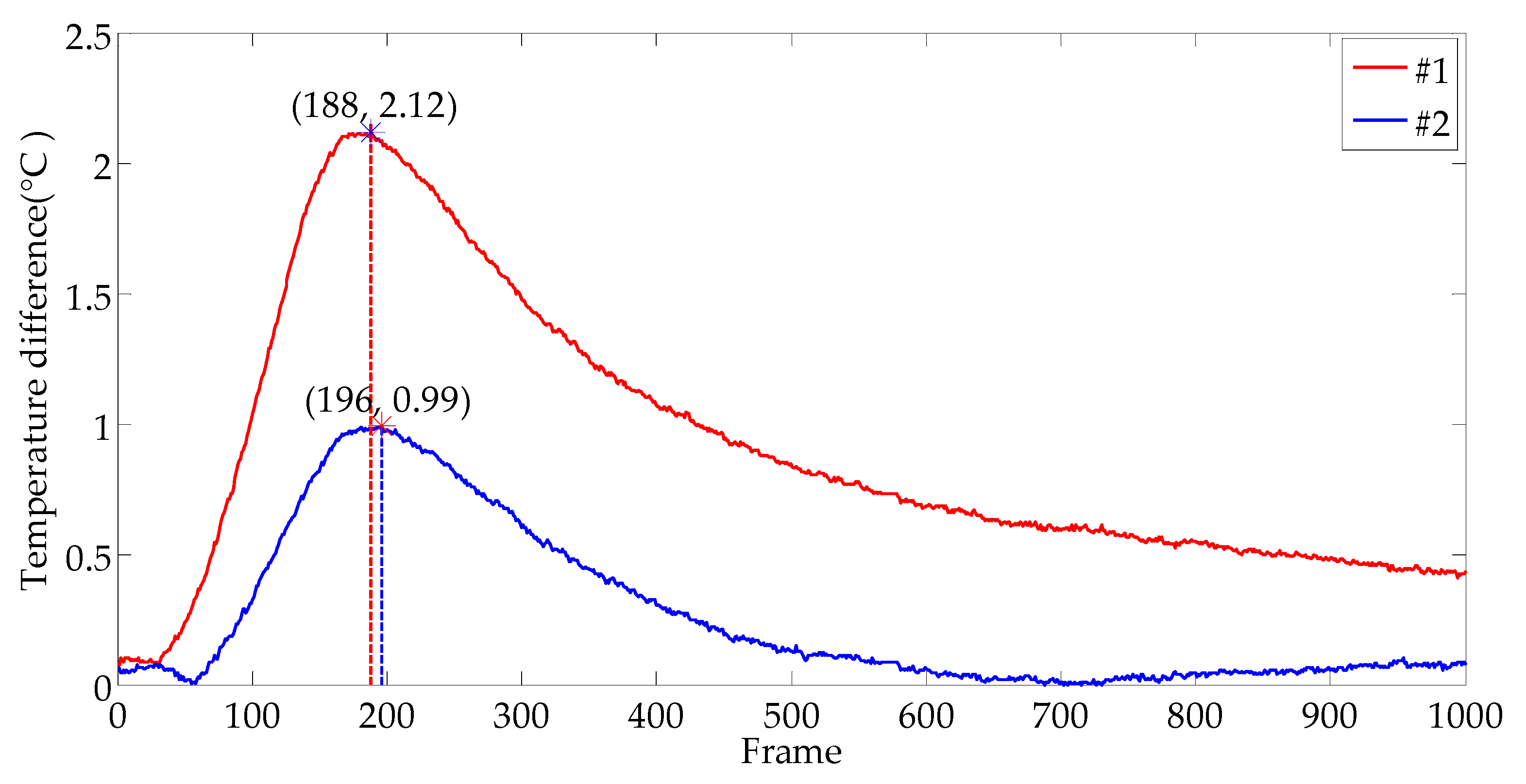
A number of sampling areas were taken at the defect area and the non-defect area to eliminate the influence of thermal excitation unevenness, as shown in Figure 25. The average temperature of different areas and the temperature difference between the defect area and non-defect area was calculated respectively, and the course curves of the average temperature difference over time were drawn, as shown in Figure 26. According to the peak values of curves, Frame 188 and Frame 196 were captured for the extraction of defects #1 and #2, respectively.
After image processing, the relative data were counted in the Table 4 and were compared with our proposed method (data in Section 4), as shown in Table 5. Both the acquired frames for each defect and their relative errors by MTDM are equivalent to the preliminary results of our proposed method (MSDSRM), and the accuracy is much lower than that of our method of secondary detection.

5.2.2. Maximum Temperature Elevation Method

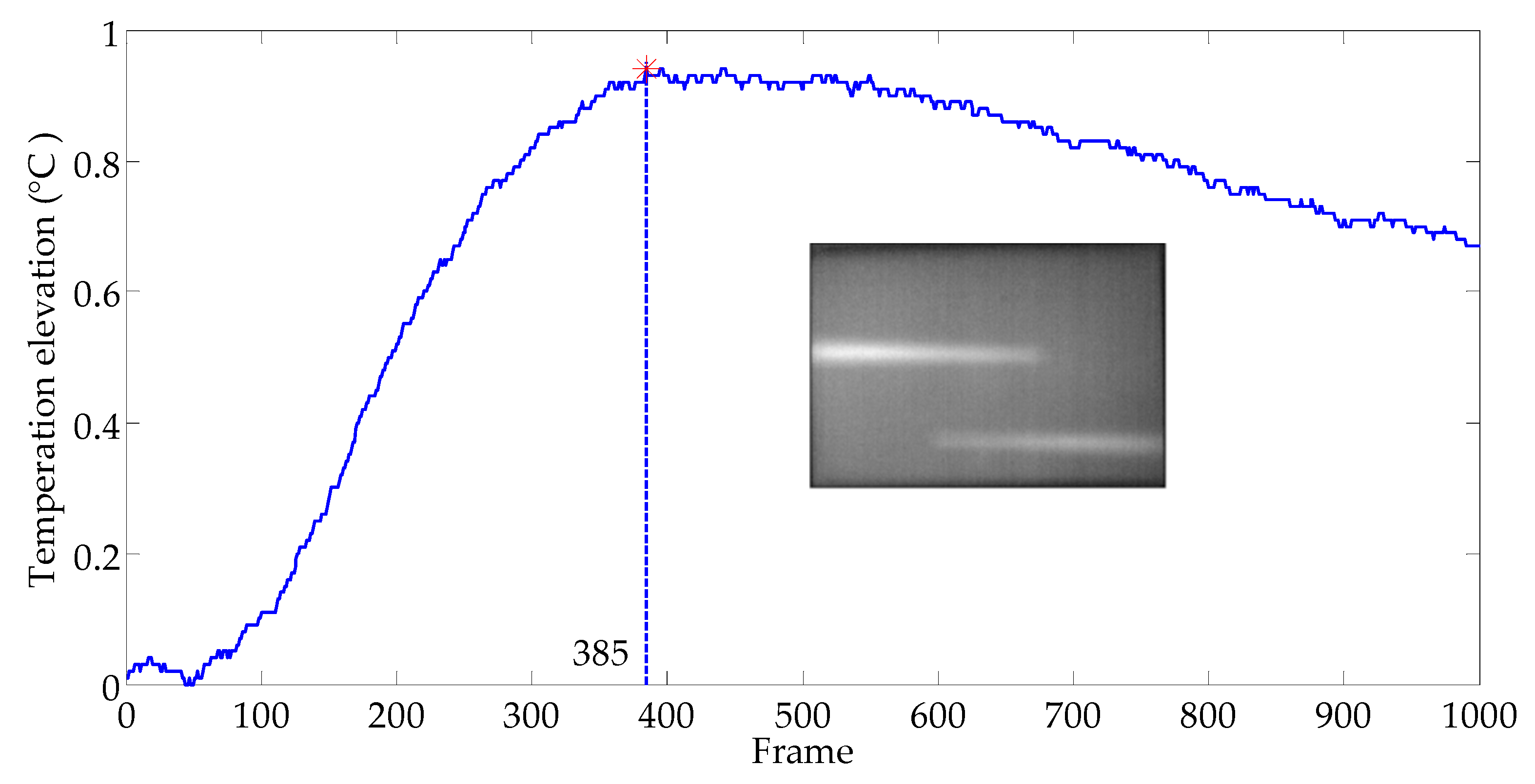
Ahmed Kabouri [6] adopted the maximum temperature elevation method (MTEM) to obtain a frame image from a sequence of thermal image for image processing. He thought that only the image acquired when the temperature reaches its maximum elevation is considered, i.e., at the time tmax corresponding to the maximum of transmitted heat and therefore a maximum of information. Using MTEM, Frame 385 was selected based on the peak of the curve of temperature elevation over time, which is presented in Figure 27. However, at Frame 385, the image has obvious heat diffusion and the defect tip has disappeared, so it is obviously not a suitable frame. Therefore, this method is not suitable for processing our sequential images.

6. Application

Carbon fiber-reinforced polymer (CFRP) has been widely used in many fields because of its excellent material properties. The impact of external energy or the mutual contact between materials will produce different degrees of impact damage on CFRP. The delamination defect inside the material is often greater than the surface damage. In this section, the method proposed by us will be used to extract the internal stratification defect of the impact damage.

6.1. Information of Specimen of Impact Damage on CFRP Laminate

6.1.1. Specimen Appearance

The size of the CFRP board is 150 mm × 100 mm × 3.89 mm. The test block is unidirectional lamination with the lamination direction [45/−45/0/−45/45/−45/45/90]. A falling weight impact test was adopted. The impact point was located at the center of the carbon fiber impact damage, and the impact energy was 72.19 J. The appearance of the impact damage is shown in Figure 28.

6.1.2. Internal Delamination Defect Detected by Ultrasonic Testing (UT)

To verify the correctness of infrared detection, the specimen was firstly detected by the ultrasonic testing of water immersion. A V312 water-immersion focused ultrasound probe was used (OLYMPUS Corporation, Japan). The piezoelectricity chip size of the ultrasonic transducer is 6.35 mm, the probe emission frequency is 10 MHz, and the focal length of the probe in water is 11.684 mm. During the experiment, the mechanical transmission controls the ultrasonic water-immersion probe to automatically scan the test block in the X and Y direction. According to the material characteristics of the specimen and the thickness of the specimen, the ultrasonic bottom echo imaging method was adopted. Set the equipment parameters as follows: the pulse voltage was 200 V, the gain of the system was set to 21 dB, the scanning speed was 40 mm/s, and the step interval was 0.2 mm. The experiment took 42 min in total. The scanning result is shown in Figure 29a. The region of interest is selected as shown in Figure 29b and the delamination defect is extracted after image processing, as shown in Figure 29c. The calculated damage area is 1836 mm2.

6.2. Impact Damage on CFRP Laminate Detected by Long-Pulse Thermography

6.2.1. Experiment of Long Pulse Thermography

The specimen of CFRP was detected by long-pulse infrared thermal wave where the detection method was the transmission method. The relevant parameters were set as follows: the pulse excitation time was 5 s, the acquisition frequency was 30 Hz, and a total of 500 frames were collected. Some frames of the sequence are shown in Figure 30.

6.2.2. Data Post-Processing with MSDSRM

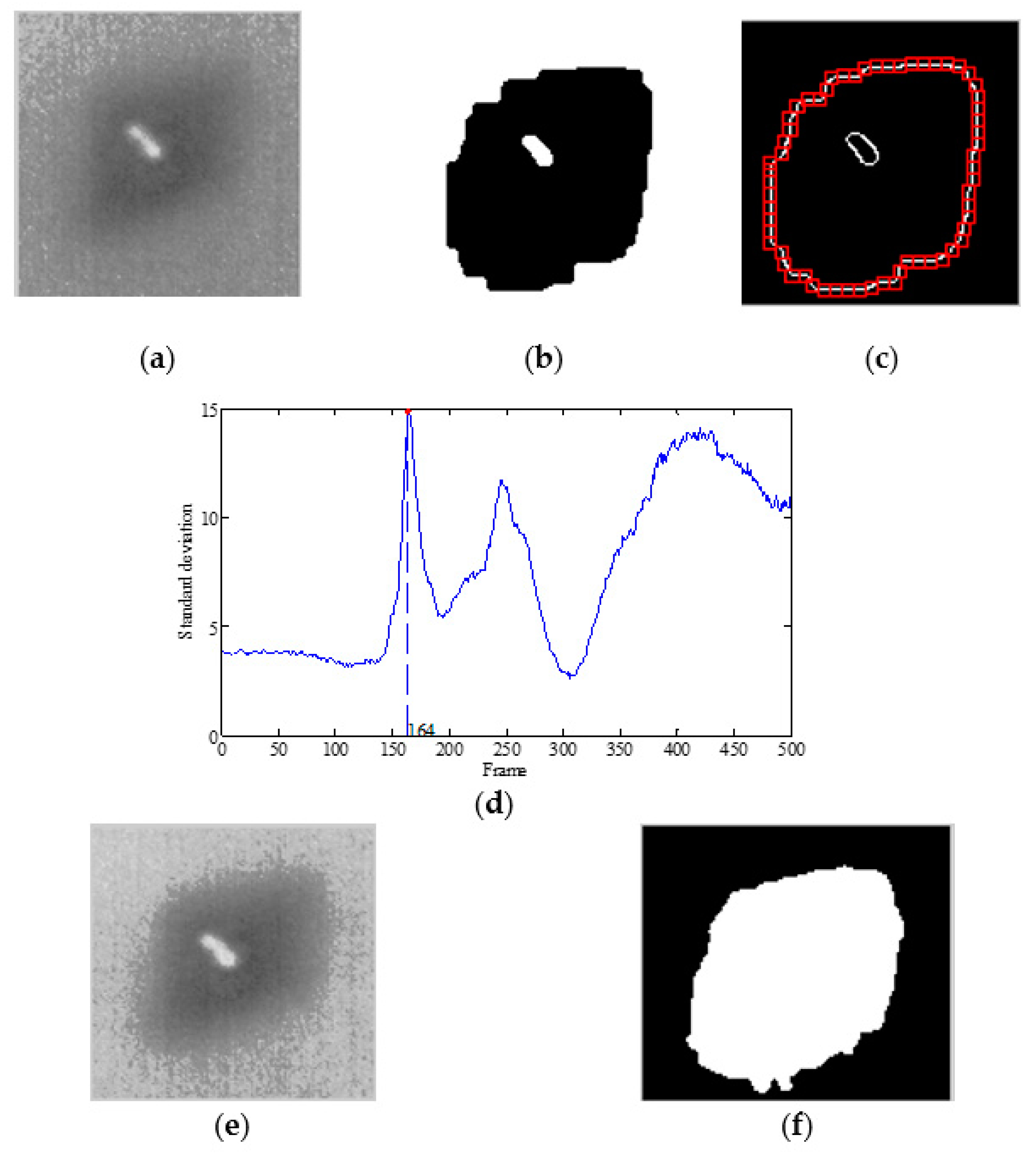
Since there is only one impact damage, blob analysis is not required. A frame is randomly selected to display the image with a relatively complete defect, such as the 150th frame, as shown in Figure 31a. The binarized image was obtained through median filtering and threshold segmentation (see Figure 31b), and then the sensitive region was located according to the extracted edge. The sensitive regions were uniformly sampled, as shown in Figure 31c. Based on the regions, the curve of the average standard deviation vs. time can be obtained, as shown in Figure 31d. We found that the variation of the curve of the CFRP specimen is more complex than the previous curve of the PVC specimen. The reason is that the structure of CFRP includes multiple layers, while PVC is single layer. According to our proposed method MSDSRM, Frame 164 was obtained at peak time, as shown in Figure 31e. At last, the defect was extracted as illustrated in Figure 31f, and the damage area was calculated to be 1765.17, which is near the value detected by UT. However, there exists some difference in the defect shape extracted by IR and by UT.

6.2.3. Data Post-Processing with MTDM

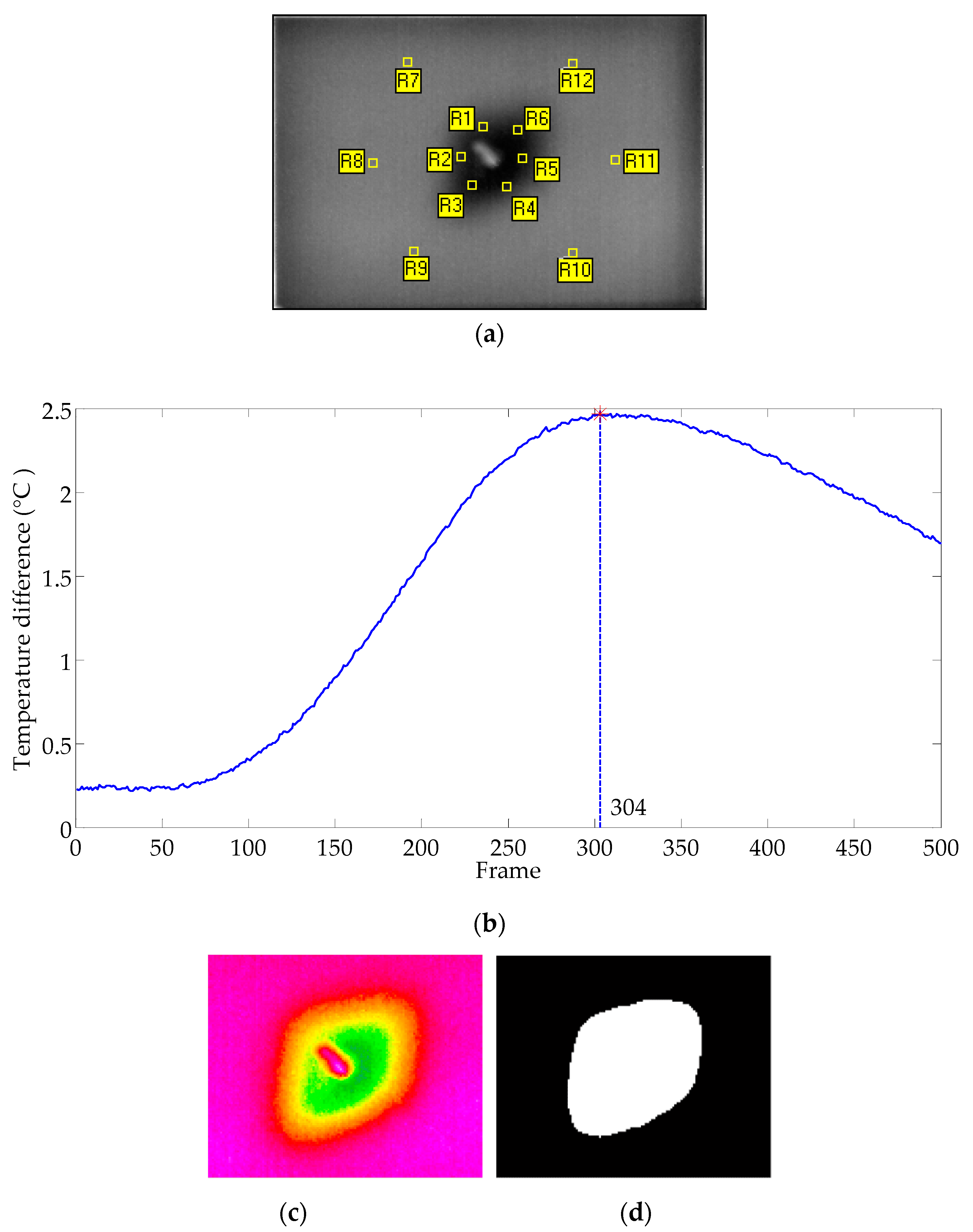
As shown in Figure 32a, there are six small regions selected for temperature sampling in the defect area and sound area in the picture, respectively. The average temperature of the two large areas is calculated respectively, and the draw temperature difference curve is presented in Figure 32b. From the figure, it can be seen that the maximum temperature difference occurs at Frame 304, so the 304th frame is captured for defect extraction. After image processing on the ROI in Frame 304 (see Figure 32c), the defect is extracted by MTDM, as shown in Figure 32d, and its shape is similar to that of Figure 31f extracted by MSDSRM, but the area of the former is smaller than that of the latter. The relevant data statistics are shown in Table 6, where the relative error is compared with the detected area 1836.99 mm2 by UT.

7. Conclusions

It is challenging to accurately acquire the defective areas with different depths on PVC materials with minimum human intervention. In this paper, we developed an effective approach to accurately detect defects with different depths on a PVC specimen. The whole process was made automatic, and no human intervention was required. We firstly quantitatively analyzed the relationships between defect depth, temperature, and time. Then, we proposed the maximum of standard deviation of the sensitive region method (MSDSRM) to decide the best frame to calculate defect boundaries, which answered a key question in thermographic defect detection. By integrating blob analysis and the Otsu method, we further proposed a fully automated process to extract defect areas. As a result, our study should offer a great help in non-destruction defect detection and quality assurance.
Further effort will be focused on extracting defects in ordinary temperature fields. For example, it may be possible to combine the MSDSRM with a temperature field processing technique such as FWHM to determine the defect size through the analysis of the surface temperature field. Furthermore, our study assumes that the infrared images have enough contrast for image processing processes such as defect contour extraction and binary segmentation, and we are aware that such a condition might not always be feasible in practice. Therefore, some pre-processing will be needed, which might affect the detection accuracy.

Author Contributions

Conceptualization, L.Y., H.L. and Y.L.; Methodology, L.Y. and P.Y.; Software, L.Y., Q.S. and H.L.; Validation, P.Y.; Formal Analysis, X.Z.; Investigation, L.Y.; Resources, L.Y.; Data Curation, X.Z.; Writing-original draft preparation, L.Y., X.Z., Q.S., P.Y. and Y.L.; Writing-review and editing, L.Y., P.Y., Q.S., and Y.L.; Supervision, L.Y., Y.L. and P.Y.; Funding acquisition, L.Y. and X.Z. All authors have read and agreed to the published version of the manuscript.

Funding

This research was funded by “Nation Natural Science Foundation of China, grant number 51865038”, “Chinese Government Scholarship for studying abroad, grant number 201708360122” and “Graduate Innovation Fund of Jiangxi Province, grant number YC2020-S547”. The APC was funded by “Nation Natural Science Foundation of China, grant number 51865038”.

Acknowledgments

This work was supported by the National Natural Science Foundation of China (Grant No. 51865038), the Chinese Government Scholarship for studying abroad (Grant No. 201708360122) and the Graduate Innovation Fund of Jiangxi Province (Grant No. YC2020-S547).

Conflicts of Interest

The authors declare no conflict of interest.

References

  1. Groz, M.-M.; Abisset-Chavanne, E.; Meziane, A.; Sommier, A.; Pradère, C. Three-dimensional reconstruction of thermal volumetric sources from surface temperature fields measured by infrared thermography. Appl. Sci. 2019, 9, 5464. [Google Scholar] [CrossRef] [Green Version]
  2. Huh, J.; Mac, V.H.; Tran, Q.H.; Lee, K.-Y.; Lee, J.-I.; Kang, C. Detectability of delamination in concrete structure using active infrared thermography in terms of signal-to-noise ratio. Appl. Sci. 2018, 8, 1986. [Google Scholar] [CrossRef] [Green Version]
  3. Fang, Q.; Maldague, X. A method of defect depth estimation for simulated infrared thermography data with deep learning. Appl. Sci. 2020, 10, 6819. [Google Scholar] [CrossRef]
  4. Oswald-Tranta, B. Comparative study of thermal contrast and contrast in thermal signal derivatives in pulse thermography. NDT E Int. 2017, 91, 36–46. [Google Scholar] [CrossRef]
  5. Tashan, J.; Al-Mahaidi, R.; Mamkak, A. Defect size measurement and far distance infrared detection in CFRP-concrete and CFRP-steel systems. Aust. J. Struct. Eng. 2016, 17, 2–13. [Google Scholar] [CrossRef] [Green Version]
  6. Kabouri, A.; Khabbazi, A.; Youlal, H. Applied multiresolution analysis to infrared images for defects detection in materials. NDT E Int. 2017, 92, 38–49. [Google Scholar] [CrossRef]
  7. Dattoma, V.; Panella, F.W.; Pirinu, A.; Saponaro, A. Advanced NDT methods and data processing on industrial CFRP components. Appl. Sci. 2019, 9, 393. [Google Scholar] [CrossRef] [Green Version]
  8. Liu, D.N.; Hou, R.; Wu, W.Z.; Hua, J.W.; Wang, X.X.; Pang, B. Research on infrared image enhancement and segmentation of power equipment based on partial differential equation. J. Vis. Commun. Image Represent. 2019, 64, 102610. [Google Scholar] [CrossRef]
  9. Wei, Y.; Su, Z.; Mao, S.; Zhang, D. An infrared defect sizing method based on enhanced phase images. Sensors 2020, 20, 3626. [Google Scholar] [CrossRef]
  10. Chrysafi, A.P.; Athanasopoulos, N.; Siakavellas, N.J. Damage detection on composite materials with active thermography and digital image processing. Int. J. Therm. Sci. 2017, 116, 242–253. [Google Scholar] [CrossRef]
  11. Deane, S.; Avdelidis, N.P.; Ibarra-Castanedo, C.; Zhang, H.; Nezhad, H.Y.; Williamson, A.A.; Mackley, T.; Maldague, X.; Tsourdos, A.; Nooralishahi, P. Comparison of cooled and uncooled ir sensors by means of signal-to-noise ratio for NDT diagnostics of aerospace grade composites. Sensors 2020, 20, 3381. [Google Scholar] [CrossRef]
  12. Li, Y.; Jin, W.; Zhu, J.; Zhang, X.; Li, S. An adaptive deghosting method in neural network-based infrared detectors nonuniformity correction. Sensors 2018, 18, 211. [Google Scholar] [CrossRef] [Green Version]
  13. Zeng, Q.; Qin, H.; Yan, X.; Yang, S.; Yang, T. Single infrared image-based stripe nonuniformity correction via a two-stage filtering method. Sensors 2018, 18, 4299. [Google Scholar] [CrossRef] [Green Version]
  14. Sripragash, L.; Sundaresan, M. Non-uniformity correction and sound zone detection in pulse thermographic nondestructive evaluation. NDT E Int. 2017, 87, 60–67. [Google Scholar] [CrossRef]
  15. Hasan, S.M.A.; Kwanghee, K. Depth edge detection by image-based smoothing and morphological operations. J. Comput. Des. Eng. 2016, 3, 191–197. [Google Scholar]
  16. Wang, D.; Wang, Z.; Zhu, J.; Ciampa, F. Enhanced pre-processing of thermal data in long pulse thermography using the Levenberg-Marquardt algorithm. Infrared Phys. Technol. 2019, 99, 158–166. [Google Scholar] [CrossRef]
  17. Liu, Y.; Tang, Q.; Bu, C.; Mei, C.; Wang, P.; Zang, J. Pulsed infrared thermography processing and defects edge detection using FCA and ACA. Infrared Phys. Technol. 2015, 72, 90–94. [Google Scholar]
  18. Jinlong, G.; Junyan, L.; Fei, W.; Wang, Y. Inverse heat transfer approach for nondestructive estimation the size and depth of subsurface defects of CFRP composite using lock-in thermography. Infrared Phys. Technol. 2015, 71, 439–447. [Google Scholar] [CrossRef]
  19. Yang, B.; Huang, Y.; Cheng, L. Defect detection and evaluation of ultrasonic infrared thermography for aerospace CFRP composites. Infrared Phys. Technol. 2013, 60, 166–173. [Google Scholar] [CrossRef]
  20. Sreeshan, K.; Dinesh, R.; Renji, K. Enhancement of thermographic images of composite laminates for debond detection: An approach based on Gabor filter and watershed. NDT E Int. 2019, 103, 68–76. [Google Scholar] [CrossRef]
  21. Wang, J.; Yuan, L.; Zhu, Z.; Yuan, M. Accurate detection of a defective area by adopting a divide and conquer strategy in infrared thermal imaging measurement. J. Korean Phys. Soc. 2018, 73, 1644–1649. [Google Scholar]
  22. Almond, D.P.; Lau, S.K. Defect sizing by transient thermography I: An analytical treatment. J. Phys. D Appl. Phys. 1994, 27, 1063–1069. [Google Scholar] [CrossRef]
  23. Tan, Y.C.; Chiu, W.K.; Rajic, N. Quantitative defect detection on the underside of a flat plate using mobile thermal scanning. Procedia Eng. 2017, 188, 493–498. [Google Scholar] [CrossRef]
  24. Kalyanavalli, V.; Ramadhas, T.; Sastikumar, D. Long pulse thermography investigations of basalt fiber reinforced composite. NDT E Int. 2018, 100, 84–91. [Google Scholar] [CrossRef]
  25. Wysock-Fotek, O.; Oliferuk, W.; Maj, M. Reconstruction of size and depth of simulated defects in austenitic steel plate using pulsed infrared thermography. Infrared Phys. Technol. 2012, 55, 363–367. [Google Scholar] [CrossRef]
  26. Duan, Y.; Zhang, H.; Maldague, X.P.V.; Ibrra-Castanedo, C.; Servais, P.; Genest, M.; Sfarra, S.; Meng, J. Reliability assessment of pulsed thermography and ultrasonic testing for impact damage of CFRP panels. NDT E Int. 2019, 102, 77–83. [Google Scholar] [CrossRef]
  27. Wu, J.-Y.; Sfarra, S.; Yao, Y. Sparse principal component thermography for subsurface defect detection in composite products. IEEE Trans. Ind. Inform. 2018, 14, 5594–5600. [Google Scholar] [CrossRef]
  28. Choi, M.; Kang, K.; Park, J.; Kim, W.; Kim, K. Quantitative determination of a subsurface defect of reference specimen by lock-in infrared thermography. NDT E Int. 2008, 41, 119–124. [Google Scholar] [CrossRef]
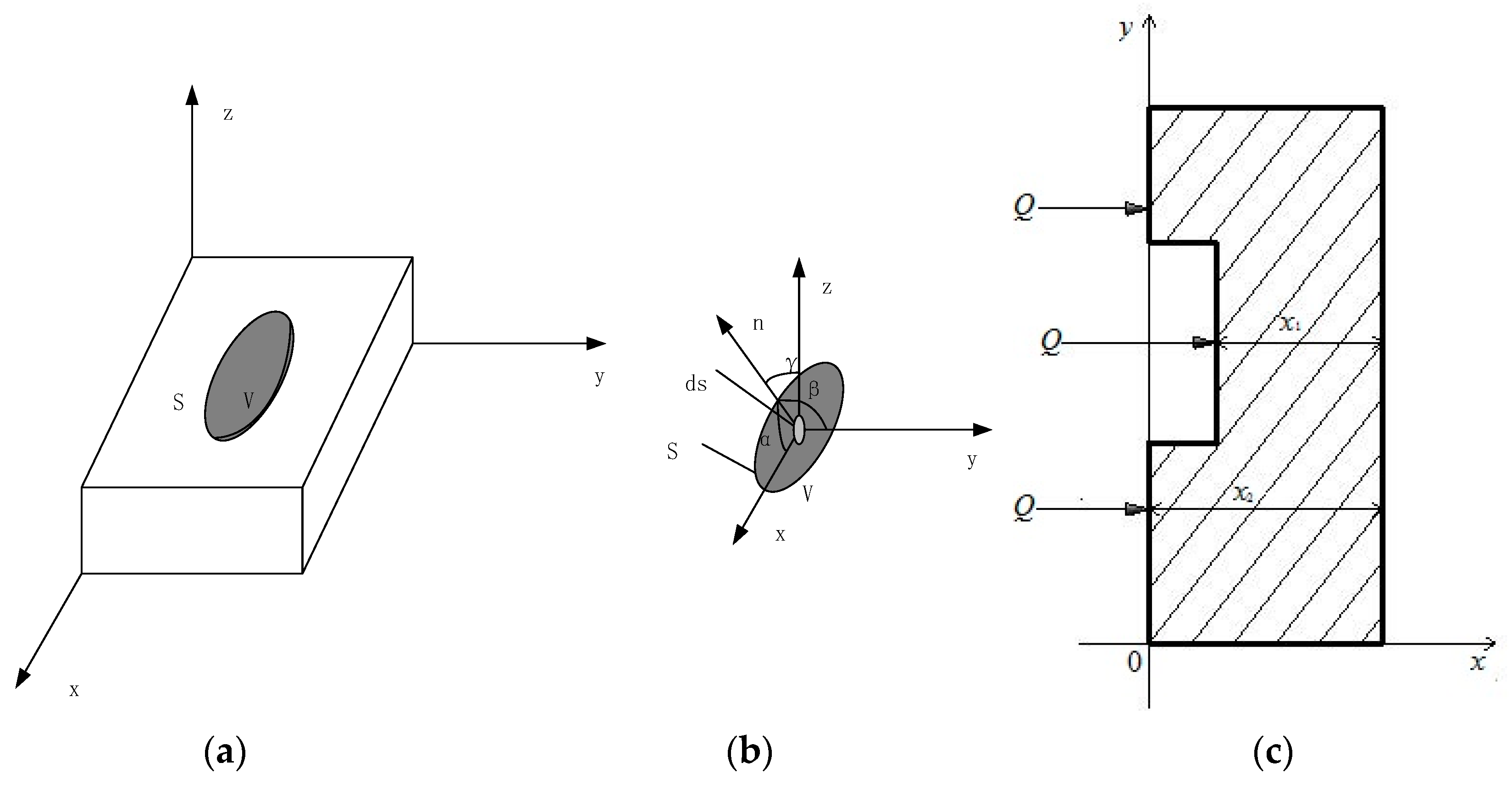
Figure 1. Schematic diagram of heat conduction theory: (a) Solid model; (b) Diagram of infinitesimal analysis; (c) A slab of specimen is excited by a pulsed heat source.
Applsci 10 08248 g001
Figure 2. Schematic diagram to illustrate the sensitive area (C) of defects (A) in the specimen (I).
Applsci 10 08248 g002
Figure 3. The history of standard deviation of the sensitive area with time.
Applsci 10 08248 g003
Figure 4. Block diagram for extraction of defects automatically and accurately.
Applsci 10 08248 g004
Figure 5. Photos of a polyvinyl chloride (PVC) test specimen: (a) The surface backs to IR camera; (b) The surface facing the IR camera.
Applsci 10 08248 g005
Figure 6. Schematics of PVC test specimen: (a) Main view: Distribution of defects; (b) Right View: Depth of defect #1; (c) Left View: Depth of defect #2.
Applsci 10 08248 g006aApplsci 10 08248 g006b
Figure 7. Synchronized infrared image acquisition system.
Applsci 10 08248 g007
Figure 8. Distribution of temperature field on the surface of the PVC test object in the sequence.
Applsci 10 08248 g008
Figure 9. The surface temperature of the shallower defect with frame.
Applsci 10 08248 g009
Figure 10. Image composition.
Applsci 10 08248 g010
Figure 11. Image processing of image composition: (a) Median filter; (b) Segmentation by Otsu’s method.
Applsci 10 08248 g011
Figure 12. Blob analysis and edge extraction in each blob: (a) Blob analysis; (b) Edge abstracted by Canny operator.
Applsci 10 08248 g012
Figure 13. Single sensitive region on each defect is randomly selected.
Applsci 10 08248 g013
Figure 14. A suitable frame for each defect is determined by the maximum of sandard deviation of sensitive region method (MSDSRM) using single sensitive region.
Applsci 10 08248 g014
Figure 15. A sketch of the region of interest (ROI) based on the blob and restrained by constraints.
Applsci 10 08248 g015
Figure 16. Defect extraction of primary detection: (a) ROI of defect #1 from Frame 178; (b) Segmentation of defect #1; (c) ROI of defect #1 from Frame 199; (d) Segmentation of defect #2; (e) Composition segmentation images as a whole.
Applsci 10 08248 g016
Figure 17. Discrete distribution of relative deviation of defect area for 100 times primary detection.
Applsci 10 08248 g017
Figure 18. Two sensitive regions selection methods: (a) Multiple sensitive areas selected uniformly; (b) 50 multiple sensitive areas selected randomly.
Applsci 10 08248 g018
Figure 19. The MSDSRM to select a suitable frame for each defect: (a) Curves of standard deviation vs. time based on uniform selection of sensitive regions; (b) Curves of standard deviation vs. time based on random selection of sensitive regions.
Applsci 10 08248 g019
Figure 20. The scatter diagram of the experiment conducted 100 times: (a) The scatter diagram of the experiment conducted 100 times by uniform selection; (b) The scatter diagram of the experiment conducted 100 times by random selection.
Applsci 10 08248 g020
Figure 21. Discrete distribution of relative deviation of defect area: (a) Discrete distribution of relative deviation of defect area using uniform selection; (b) Discrete distribution of relative deviation of defect area using random selection.
Applsci 10 08248 g021
Figure 22. The maximum standard deviation surface related to width and height: (a) The maximum standard deviation surface for #1; (b) The maximum standard deviation surface for #2.
Applsci 10 08248 g022
Figure 23. The 3D scatter diagram of selection frames with the sensitive region size variation: (a) The 3D scatter diagram of selection frames for #1; (b) The 3D scatter diagram of selection frames for #2.
Applsci 10 08248 g023
Figure 24. The scatter diagram of the experiment conducted 100 times to be compared with Figure 19: (a) The scatter diagram of the experiment conducted 100 times by uniform selection; (b) The scatter diagram of the experiment conducted 100 times by random selection.
Applsci 10 08248 g024aApplsci 10 08248 g024b
Figure 25. Schematic diagram of defect area and sound area sampling.
Applsci 10 08248 g025
Figure 26. The curves of average temperature difference between the defect area and sound area over time.
Applsci 10 08248 g026
Figure 27. The curve of average temperature elevation over time and the acquired frame image.
Applsci 10 08248 g027
Figure 28. The specimen of impact damage of carbon fiber-reinforced plastics (CFRP).
Applsci 10 08248 g028
Figure 29. Delamination defect detected by UT and its extraction: (a) Delamination defect detected by UT; (b) ROI; (c) Defect segmentation.
Applsci 10 08248 g029
Figure 30. Delamination defect detected by long-pulse thermography.
Applsci 10 08248 g030aApplsci 10 08248 g030b
Figure 31. Delamination defect extracted by MSDSRM: (a) ROI of Frame 150; (b) Binary image; (c) Sensitive areas selected; (d) Curves of standard deviation vs. time based on random selection of sensitive regions; (e) ROI of Frame 164; (f) Defect segmentation.
Applsci 10 08248 g031
Figure 32. Delamination defect extracted by MTDM: (a) Schematic diagram of defect area and sound area sampling; (b) The curves of average temperature difference between the defect area and sound area over time; (c) ROI in Frame 304; (d) Defect extraction.
Applsci 10 08248 g032
Table 1. Statistics of defect parameters on image composition processing.
Defect NumberObjectThresholdDefect NumberDefect PixelRelative Error
#1Image composition0.47#14286.527.08%
#2#22188.334.47%
Table 2. Statistics of defect parameters using a single sensitive region.
Defect NumberFrameThresholdDefect PixelRelative Error
#11780.463443.12.08%
#21990.363242.12.91%
Table 3. Statistics of defect parameters using multiple sensitive regions.
Defect NumberUniform SelectionRandom Selection
FrameDefect PixelRelative ErrorFrameDefect PixelRelative Error
#11643404.70.94%1663384.20.33%
#21833420.82.44%1863430.52.73%
Table 4. Statistics of defect parameters using the maximum temperature difference method.
Defect NumberFrameThresholdDefect PixelRelative Error
#11880.423525.54.52%
#21960.443191.94.42%
Table 5. Compared the results of MSDRM with those of maximum temperature difference method (MTDM) for PVC specimen.
Defect NumberMSDSRMMTDM
Single SelectionMultiple Uniform SelectionMultiple Random Selection
FrameErrorFrameErrorFrameErrorFrameError
#1(158, 193)[0.25%, 4.94%]1640.42%(164, 173)[0.24%, 1.06%]1884.52%
#2(160, 203)[1.05%, 5.37%]182,183,186[0.94%, 2.44%](173, 193)[0.47%, 3.15%]1964.42%
Table 6. Comparison of the results of MSDRM and MTDM for CFRP specimen.
MethodFrameDefect PixelArea (mm2)Relative Error
MSDSRM1646073.61765.173.91%
MTDM3043298.8958.7347.81%
Publisher’s Note: MDPI stays neutral with regard to jurisdictional claims in published maps and institutional affiliations.