Wind Reversal in Bubbly Natural Convection

Abstract

The multi-phase Rayleigh–Bènard convection has been weakly investigated, even though it plays a leading role in the theoretical and applied physics of the heat transfer enhancement. For the case of moderate turbulent convection, a rather unexpected result is an unusual kind of wind reversal, in the sense that the fluid is found to be strongly influenced by the bubbles, whereas the bubbles themselves appear to be little affected by the fluid, despite the relative smallness of the Stokes numbers. The wind reversal induced by the bubbles dispersed in the fluid is a new and remarkable phenomenon in multi-phase flows that provides further perspectives in understanding the complex physics leading the enhancement of thermal convection. For this reason, the fundamental research proposed in this paper aimed to identify a space of control parameters and the physical mechanisms responsible for the wind reversal induced by dispersed bubbles in a confined convective flow. The strength of the following description lies in an innovative numerical approach, based on the multi-scale physics induced by the coupling of the local thermal and mechanical mechanisms arising between each bubble and the surrounding fluid. The continuous phase has been solved numerically using the direct numerical simulation (DNS) technique and each bubble has been tracked by means of a particle Lagrangian model.

1. Introduction

The standard Rayleigh–Bénard convection occurs in a Newtonian single-phase fluid, bounded by lower (hot) and upper (cold) horizontal plates both at constant temperature, and an adiabatic side-wall. The thermal-induced buoyancy force pushes the stream toward the hotter region where the fluid is lighter. In the colder region, it happens in exactly the opposite way. The thermal convection undergoes significant changes with phase transitions [1,2] and when polymers [3], bubbles [4,5], and particles [6] disperse in the continuous phase. The most relevant effect is the heat transfer enhancement of the multi-phase convection respect to the case of single phase convection.

The multi-phase Rayleigh–Bénard convection plays a leading role in a wide range of physical phenomena such as the formation of atmospheric precipitation [7], magma chambers [8,9] boiling of liquid [10], and counterflow cooling towers [11].

It is well known that suspended particles or bubbles have a very strong effect on turbulent flows. A considerable amount of experimental evidence has been accumulating for more than 40 years, showing that small particles or bubbles dampen the turbulence, while larger ones increase it, due to vortex shedding behind them [12]. The particles selectively interact with the coherent structures and, in turbulent flows, they preferentially distribute avoiding strong vortical regions whereas they clustering tight regions [13,14]. The near-wall turbulent vortical structures control the transport of the particles and the mechanisms that finally segregated them within the viscous boundary layer [15].

All these insights can be used only to roughly depict the physics leading the bubbles turbulence interaction in convective flows. Indeed, the multi-phase convection shows a wide richness of multi-scale physics due to the interplay of the isotropic turbulence in the bulk [16] with the viscous and thermal boundary layers [17] and with the local intermittent events such as the thermal plumes [18]. In such a system, the dispersed phase interacts with the various temporal and spatial scales of the flow topologies according to the coupling of local thermal and mechanical interact between each particle and the surrounding fluid. The physics of particles and bubbles dispersion in convective flows is a key feature in understanding the turbulence dampening and the enhancement of the thermal convection [4,5,6].

The control parameters governing the Rayleigh–Bénard convection under the Boussinesq approximation are the Rayleigh number Ra (ratio between buoyancy and viscous forces), the Prandtl number Pr (ratio between the thicknesses of the thermal and viscous boundary layers), and the aspect ratio of the geometrical domain; the response parameter is, instead, the Nusselt number (heat transfer rate). In the turbulent regime, the flow is characterized by a large-scale circulation (LSC).

The LSC, often called mean wind, whose scale is of the same order of magnitude of the container, overlaps with the background turbulence [19]. The mean wind seems to persist at least for several dozens of the Rayleigh number and for a variety of Prandtl numbers. This wind is fed and driven by the thermal plumes detaching from the boundary layers but also acts back onto the plume formation process [20,21]. The temperature fluctuations in the thermal layer is responsible for the generation of the thermal plumes [22]. In the literature, there is not a precise definition for the thermal plume, but we can follow what we find in Ching et al. [23], that defined the plume like a coherent structures arising from the thermal boundary layers by buoyancy. The plume makes the strain high because of the sweeping connected to the rising of hot fluid. The operative methodologies, able to identify the thermal plume, are mainly based on: (i) the characterization of the coherent structures in the boundary layers and (ii) the analysis of the thermal fluctuations of the local measurements. In the 1990s, the fly-wheel picture was developed for the large-scale wind.

In recent years, however, it has become clear that at least in cylindrical Rayleigh–Bénard cells (aspect ratio of order one) the internal dynamics of the wind is more complicated: the horizontal direction of the wind near the thermal plate oscillates in time [24]. This is remarkable as the driving buoyancy has a vertical component only. The temporal correlation of the wind direction oscillations is found to be very long, namely, hundreds of large eddy turnover time. Beyond the horizontal oscillation, the large-scale wind selects a vertical plane at a new azimuthal position after that the cessation occurs. In comparison with the dynamics of the large-scale wind, this cessation scenario is rare.

For very large Rayleigh numbers, the large scale wind may even break down, as the driving plumes may have cooled down before they reach the other side of the cell. The change in the features of the mean flow has also influence on the boundary layers dynamics [25]. The thermal boundary layer thickness decreases steadily with Ra, the viscous boundary layer also decreases but not linearly, showing a clear thickening produced by the different mean flow.

An important feature is the different of values, in the bulk and in the boundary layers, of the kinetic energy dissipation rate ${ϵ}_k$ and the temperature dissipation rate ${ϵ}_T$. Although it attains the largest values in the boundary layer, the dissipation in the bulk is not negligible too; thus, due to the small volume of fluid in the boundary layers the bulk dissipation dominates. By contrast, the temperature in the bulk, ${ϵ}_T$, is a negligible fraction of that at wall and essentially all the ${ϵ}_T$ are produced within the thermal boundary layers.

The strength of the numerical approach is the multi-scale physics induced by the coupling of local thermal and mechanical interactions between each particle and the surrounding fluid. For this purpose, the standard point-particle model has been extended in order to interact with the thermal effects associated with the thermal balance at the particle surface. A significant difference respect to the single-phase numerical method lies in the new source terms introduced in the momentum and in the thermal energy equations. The time integration of the Navier–Stokes equations with the Boussinesq approximation and the Lagrangian particle equations takes into account the Kolmogorov time scales, the particle relaxation time for the momentum and the thermal balance. A new feature is a further constraint on the time step since the particle moves through the viscous and the thermal boundary layers with a sequence of thermal and mechanical equilibrium states with the surrounding fluid. The numerical results are in good agreement with experiments in the case of bubbly convection reported in [26]. The solver handles the multi-dispersed particle distribution and it is parallelized by OpenMp for both the Eulerian continuum phase and the Lagrangian particle tracking.

2. Methods

In a cylindrical domain, $7.5\times {10}^3$ bubbles were inserted so that each of them gets a random value for its initial position. The cylindrical domain is $17.9$ mm height (H) with diameter of $D=8.95$ mm and aspect ratio $\Gamma =D/H=0.5$. The cold temperature at the lower plate is $T_c$ and the hot temperature at the upper plate is $T_h$, which is $\Delta T=T_h-T_c=0.25$ K, whereas the dimensionless temperature is $\psi =(T-T_c)/(T_h-T_c)$. The characteristic free fall velocity is $U_f=\sqrt{g\beta (T_h-T_c)H}$ and it is used to adimensionalize the velocities. The length scale is the height of the domain H and the time scale is $\tau =H/U_f$. The number of bubbles is constant and it is equal to $N_b={10}^5$. The bubbles change their volume because of the hot temperature and the maximum void fraction is equal to $5\times {10}^{-3}$.

The main control parameters for the bubbles size, whose initial diameter is equal to 25 $\mathsf{\mu }$m, are the Stokes number $S{t}_f=2.94\times {10}^{-5}$, the Froud number $Fr=\sqrt{1.88}\times {10}^{-2}$, and the Jakob number $Ja=1.2\times {10}^{-1}$. They disperse in a stationary convective flow with Rayleigh number $Ra=2\times {10}^5$ and Prandtl number $Pr=1.65$ (water at a temperature of 373 K and atmospheric pressure) in order to investigate the change of the flow without background turbulence but subjected to a thermal gradient.

2.1. Continuum Phase

We solve the continuity, momentum, and energy equations in a cylindrical domain with a No-slip condition applied to the all solid surfaces. The temperatures of the top and bottom surfaces are kept constant at $T_c$ and $T_h$, respectively, while the lateral boundary is assumed to be adiabatic.

The Navier–Stokes equations are solved in a cylindrical coordinate system using a second-order, finite difference, fractional-step method on a staggered grid.

$$\nabla ·\mathbf{u}=0$$

(1)

in which u is the liquid velocity field. The momentum equations is

$$\rho \frac{D\mathbf{u}}{Dt}=-\nabla p+\mu {\nabla }^2\mathbf{u}+\beta \rho (T-T_{sat})g+\sum _i{\mathbf{f}}_i\delta (\mathbf{x}-{\mathbf{x}}_i)$$

(2)

where $D/Dt$ is the convective derivative, p and T are the pressure and temperature, and $\mu =\nu \rho$ the dynamic viscosity. The continuity equation reads as in Equation (1) in the case of small bubble volume fraction.

The Navier–Stokes equations are solved using a finite difference numerical code in cylindrical coordinates based on direct numerical simulation (DNS). Direct numerical simulation is a methodology in computational fluid dynamics in which the whole range of spatial and temporal scales of the coherent structures are resolved without any turbulence model. The flow field is calculated by means of the fractional step method and an approximate-factorization technique, in which the non-linear terms are treated explicitly, whereas the viscous terms are computed implicitly. The fractional step is a method of approximation of the evolution equations based on the decomposition of the operators. The role played by the pressure is a projection operator that projects an arbitrary velocity field into a divergence-free velocity field. The general procedure for projection methods is a predictor–corrector approach. In the first step, a preliminary velocity field is computed using the momentum equation. This velocity does not satisfy the continuity equation because in this step the pressure value is not updated. In a second step, a Poisson-type equation for the pressure is solved, which is derived using the continuity equation. In the last step, the preliminary velocity field is projected in a divergence-free velocity field using the computed pressure [27]. We used the second-order explicit Adams–Bashforth scheme for the convective terms and the second-order-implicit Crank–Nicholson scheme for the viscous terms. Implicit treatment of the viscous terms eliminates the numerical viscous stability constraint. This constraint is strong for the flow with low-Reynolds number and it is relevant near boundaries where stretched meshes are used. The implicit treatment of the viscous terms requires the inversion of large sparse matrices. In order to face this numerical problem, the viscous terms are split into three tridiagonal matrices by a factorized procedure. The time advancement of the solution is obtained by a 3rd order Runge–Kutta. The simulations were carried out using a grid with 33 × 25 × 80 nodes in the azimuthal, radial and axial directions, respectively. We checked the grid resolution with a finer grid of 33 × 40 × 120 nodes finding differences in the value of the Nusselt number within $1.5\%$, [28]. Moreover, the viscous and the thermal layers were resolved since the points clustered toward each boundaries are 15 in the case of single phase flow and 6 in the case of multi-phase flow.

2.2. Dispersed Phase

The bubbles were considered to be point-like.

The single bubble is located at the coordinate ${\mathbf{x}}_i$ and the force ${\mathbf{f}}_i$ that it induce on the continuum phase reads as follows:

$${\mathbf{f}}_i=\frac{4}{3}\pi R_{bi}^3\rho \left({\left.\frac{D\mathbf{u}}{Dt}\right|}_{{\mathbf{x}}_i}-\mathbf{g}\right)$$

(3)

in which $R_{bi}$ is the radius of the i-th bubble.

The continuum phase energy equation is:

$$\rho c_p\frac{DT}{Dt}=k{\nabla }^{2}T+\sum _i{Q}_i\delta (\mathbf{x}-{\mathbf{x}}_i)$$

(4)

where $k=\kappa \rho c_p$ is the liquid thermal conductivity and $Q_i$ is the energy source or sink due to phase change of the i-th bubble.

We take into account the thermal balance between each bubble and the surrounding fluid by means of a heat transfer coefficient $h_{bi}$

$$Q_i=4\pi R_{bi}^2{h}_{bi}(T_{sat}-T_i)$$

(5)

where $T_i=T({\mathbf{x}}_i,t)$ is the liquid temperature evaluated at the position of each bubble center. In the previous equation we assume that the phase change is slow and the temperature at the bubble surface is kept at the saturated conditions.

The equation of motion for each bubble balances added mass, drag, lift and buoyancy,

$$\begin{array}{ccc}& & C_A\frac{d\mathbf{v}}{dt}=(1+C_A)\frac{D\mathbf{u}}{Dt}-\frac{3C_A}{R_b}(\mathbf{v}-\mathbf{u})\frac{d{R}_b}{dt}\hfill \\ & & -\frac{3}{8}\frac{C_D}{R_b}|\mathbf{v}-\mathbf{u}|(\mathbf{v}-\mathbf{u})-\mathbf{g}\hfill \\ & & +C_L(\nabla \times \mathbf{u})(\mathbf{v}-\mathbf{u})\hfill \end{array}$$

(6)

in which $C_A$, $C_L$, and $C_D$ are the added mass, lift, and drag coefficients, respectively. The bubble radius $R_b$ is calculated by balancing the latent heat associated to evaporation or condensation with the heat exchanged with the liquid

$$\frac{d{R}_b}{dt}=\frac{h_b}{L{\rho }_V}(T-T_{sat})$$

(7)

in which ${\rho }_V={\rho }_V\left(T_{sat}\right)$.

We take $C_A=1/2$, the standard potential-flow value for a sphere and we model the drag coefficient as suggested by [29]:

$$C_D=\frac{16}{R{e}_b}\left[1+\frac{R{e}_b}{8+\frac{1}{2}(R{e}_b+3.315\sqrt{R{e}_b})}\right]$$

(8)

in which $R{e}_b=2R_b|\mathbf{v}-\mathbf{u}|/\nu$ is the bubble Reynolds number.

The equation of the dispersed phase and continuum phase are solved numerically according to the following procedure:

Upon integration of the fluid momentum and energy equations over a computational cell, the effect of the particles is localized at their position and this effect must be replaced by an equivalent one located at the computational nodes. This task is achieved by a second-order-accurate interpolation. The interpolation preserves the resultant and the couple of the particle forces, as well as the total amount of heat that each particle exchanges with the fluid. The numerical integration of the dispersed phase follows three steps:

(i) the equation of the thermal balance at the vapor surface is solved by means the 2nd order Adam–Bashfort scheme and the radius of the bubble is updated; (ii) the momentum equation is solved using the 2nd order Adam–Bashfort scheme too, whereas the implicit 2nd order Crank–Nicholson method has been used for the drag force (iii) the bubble position is updated by Adam–Bashfort 2nd order. The implicit 2nd order scheme for the bubble momentum equation makes the solution stable with the smallest bubbles since they have a fast time evolution.

When a bubble reaches the top of the cell, it is removed from the calculation and a new bubble is re-injected at a random position on the bottom plate with a velocity equal to that of the surrounding fluid.

Each bubble is injected with its initial diameter as it is not estimated using any nucleation model. The mesh independence study and both the experimental and numerical validations were reported in Lakkaraju et al. [26]. More details were reported by the authors—in the numerical code by Oresta et al. [28].

3. Results

3.1. Convection Enhancement Induced by Vapor Bubbles Nucleation

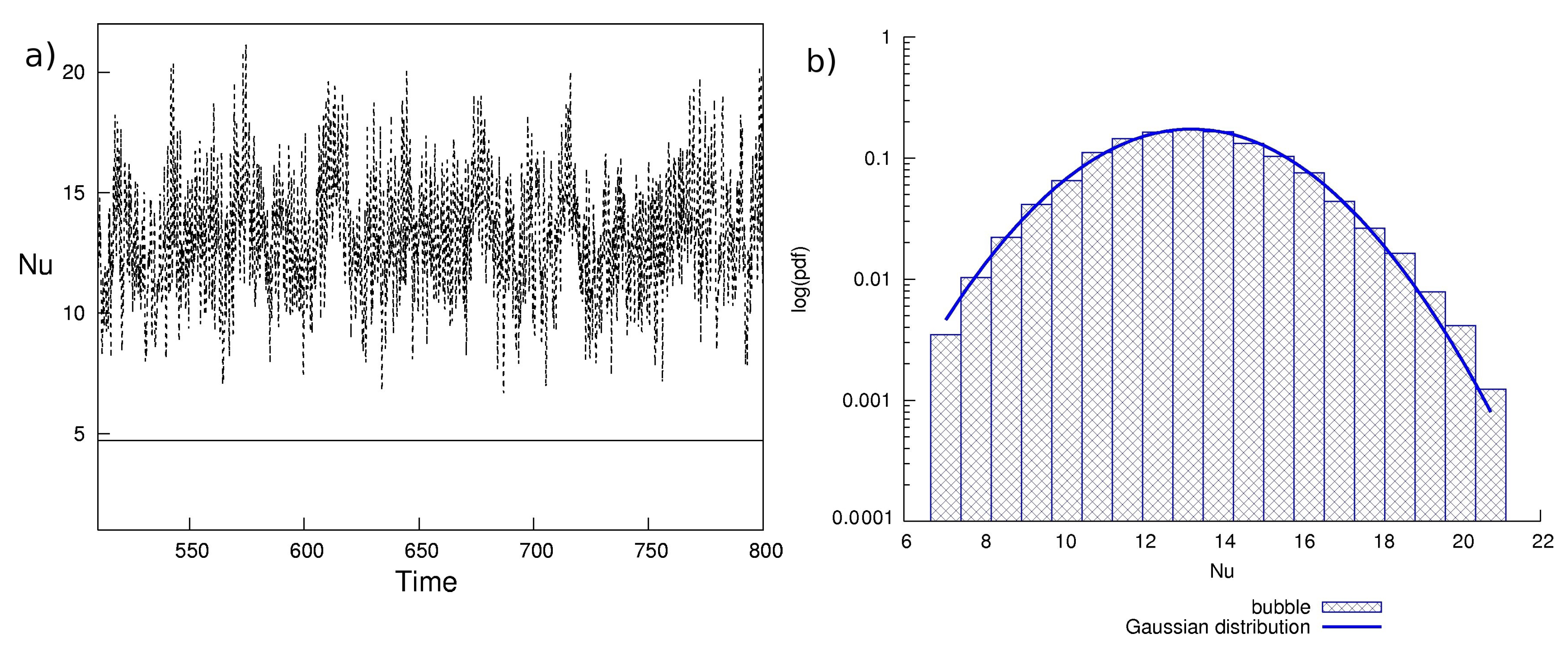
The control parameter quantifying the convection is the time evolution of the Nusselt number $Nu$ (heat flux transferred through the plates normalized by its purely conductive value) as shown in Figure 1. No bubbles flow manifested itself with a single roll that fills the whole domain and the Nusselt number shows a stationary behavior with a constant value equal to 4.718. Such a laminar flow gets highly non-stationary behavior induced by the dispersion of vapor bubbles nucleated at the bottom plate. The rising motion of bubbles increases the fluid energy in terms of both momentum and heat. Those enhancements of the flow energy flow are function of the Jakob number.

The Jakob number is a dimensionless parameter that takes into account the bubble ability to increase its own volume due to the heat transfer with the surrounding fluid. To increase the Jakob number, the bubbles enlarge more and more, traveling in the vertical direction towards the upper plate. Under this condition, the presence of bubbles increases the time averaged Nusselt number from 4.718 (no bubble flow) to 13.13 (two-way coupling flow). It should be pointed out that the bubble becoming bigger compared to its initial size changes its dynamics, which can be described by means of the point-like approximation. Moreover, the bubbles are responsible of the fluctuations in time of the Nusselt number, as their irregular rising motion generates small vortical structures characterized by highly non-stationary regime with high frequencies of the control parameter signal.

The dispersion of bubbles causes a strongly non-linear change in the heat transfer. In Figure 1 two flow cases, with and without bubbles, are shown for a computational domain with aspect ratio $\Gamma =1/2$. The average value of the heat transfer trend of the flow with bubbles is much enhanced, with respect to non bubble flow and it is worth noting how the fluctuations determined the transition to a turbulent-like behavior. In Figure 1b, the probability density function of the Nusselt number fluctuations is shown

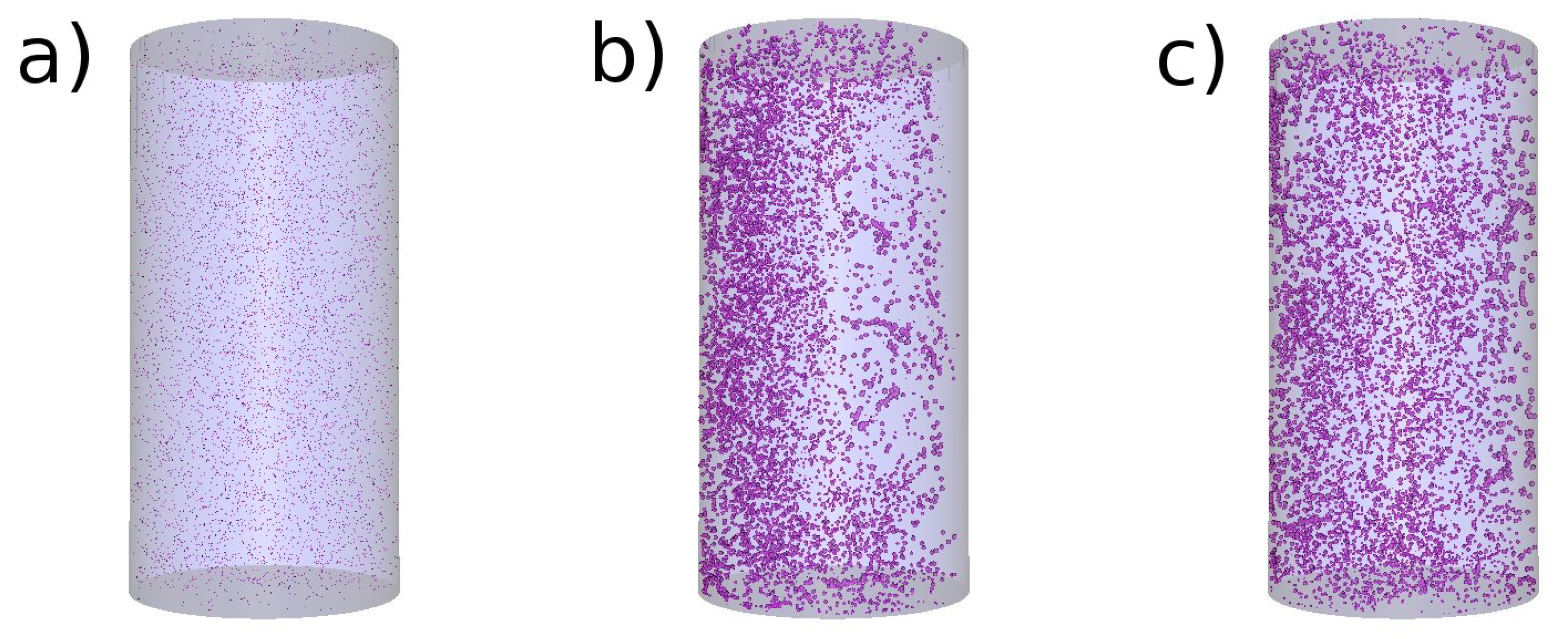
As we see, the probability density function of Nu nicely agrees with the Gaussian distribution. This statement underline the role played by the rare events of the distribution tail superimposed to the mainstream circulation. The rare events due to the nucleation, growth, and rising motion of the bubbles, are independent because ruled by the Gaussian distribution. The bubbles are not clustered by the flow if we consider the average time at which any random configuration is allowed. Instead, if we look at the instantaneous displacement of the bubbles (Figure 2) they are preferentially located into the ascending stream.

How can the bubbles behave differently? The answer is in the wind reversal, which instantaneously pushes the particles to the ascending stream, but also sweeps over the azimuthal direction, and in doing so, avoiding any preferential marker in the average thermodynamical parameters. In fact, they follow the Gaussian distribution such as the Nusselt number.

The following investigation was based on the evidence that the Nusselt number shows higher frequencies mainly because of small structures induced by the bubbles rather than the large-scale circulation.

3.2. Wind Reversal: Detection and Analysis

The bulk dynamics is characterized by the angular orientation ${\theta }_c$ of the large-scale circulation (LSC) plane and by the amplitude of the temperature fluctuation $\delta$ in the azimuthal direction. Typically, $\delta$ is a measure of the magnitude of the LSC.

Taking advantage of the data accessibility provided by the direct numerical simulation, the flow dynamics were explored.

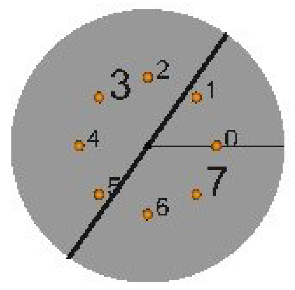
Several numerical probes are placed within the fluid volume, allowing point-wise velocity and temperature time series to be extracted. The eight probes (Figure 3) are located along the azimuthal direction every $\pi /4$ rad starting from ${\theta }_0=0$ rad on the horizontal plane midway between the two plates (cold and hot) at a radial location $r/H=0.125$ (where, r the radial coordinate and H the height of the cylindrical domain).

According to Brown et al. [30], we fitted the adimensional probe temperature ${\psi }_i$ i = 0, ...7, separately at each time, using the following function:

$${\psi }_i^{*}={\psi }_m+\delta cos(i\pi /4-{\theta }_c)$$

(9)

where ${\psi }_m=1/8{\sum }_{i=0}^7{\psi }_i$ is the average temperature of the eight probes. The $\delta$ and ${\theta }_c$ are estimated by enforcing the minimum of the square error function $E{r}_{\psi }={\sum }_{i=0}^7{({\psi }_i^{*}-{\psi }_i)}^2$. In order to avoid the non-linearity of the error function due to the cosine of ${\theta }_c$ (coming from Equation (9)), that equation is rewritten as follows.

$${\psi }_i^{*}={\psi }_m+A·sin(i\pi /4)+B·cos(i\pi /4);\delta =\sqrt{A^2+B^2},{\theta }_c=arctg\left(\frac{A}{B}\right)$$

(10)

$$\left\{\begin{array}{c}{\displaystyle E{r}_{\psi }=\sum _{i=0}^7{({\psi }_i^{*}-{\psi }_i)}^2}\hfill \\ \\ {\displaystyle \frac{\partial E{r}_{\psi }}{\partial A}=0}\hfill \\ \\ {\displaystyle \frac{\partial E{r}_{\psi }}{\partial B}=0}\hfill \end{array}\right.⟹\hspace{1em}\left\{\begin{array}{c}{\displaystyle A=\frac{1}{4}\sum _{i=0}^7{\psi }_{i}sin\left(i\frac{\pi }{4}\right)}\hfill \\ \\ \\ \\ {\displaystyle B=\frac{1}{4}\sum _{i=0}^7{\psi }_{i}cos\left(i\frac{\pi }{4}\right)}\hfill \end{array}\right.$$

(11)

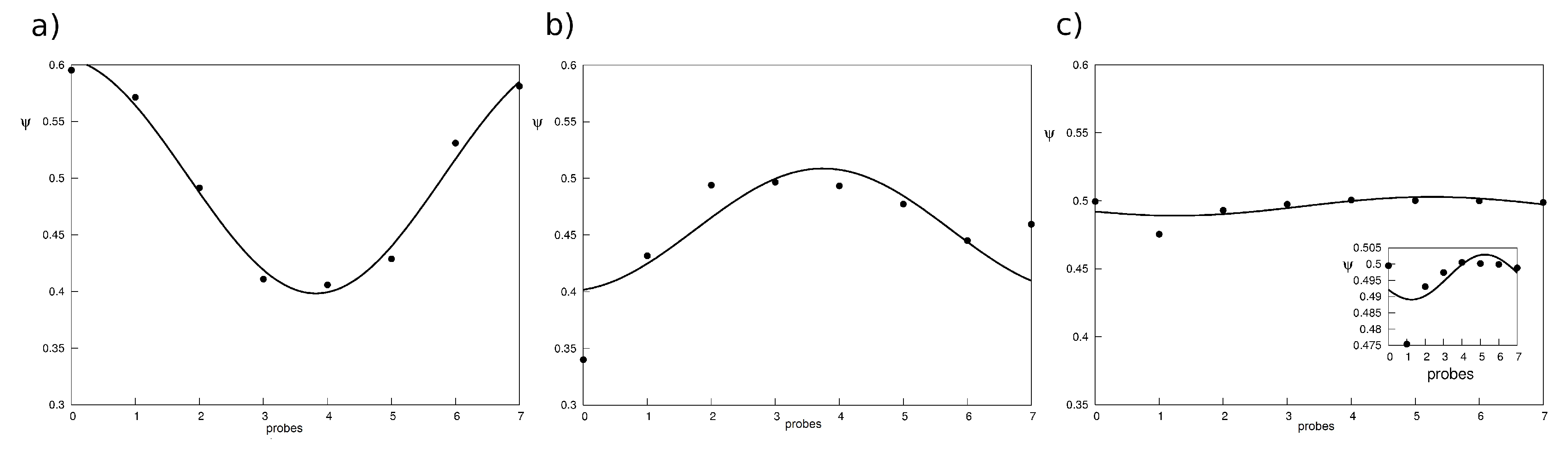
Figure 4 shows the ${\psi }_i$ and the corresponding fit ${\psi }_i^{*}$ at three time instants with Figure 4a corresponding to the beginning of the phenomenon. The parameters ${\psi }_m$, $\delta$ and ${\theta }_c$ have been listed in

Table 1. Parameters values of the fit function ${\psi }_i^{*}$ at three time instants. The time (T) is adimensionalized by means of the free fall velocity and the height of the cylindrical domain.

Dimensionless Time	${\mathit{\psi }}_{\mathit{m}}$	$\mathit{\delta }$	${\mathit{\theta }}_{\mathit{c}}$
500.0	$5.019\times {10}^{-1}$	$1.037\times {10}^{-1}$	6.141
521.8	$4.547\times {10}^{-1}$	$5.404\times {10}^{-2}$	2.942
530.0	$4.960\times {10}^{-1}$	$6.910\times {10}^{-3}$	4.124

.

The fitted temperature ${\psi }_i^{*}$ shows a good agreement with the sampled temperature ${\psi }_i$ sampled; moreover, we observe that $\delta$ and ${\theta }_c$ are strongly dependent on time.

The reorientation of the LSC was observed in turbulent convection but its dynamics is still only partially understood. An interesting aspect of the LSC observed in literature is its spontaneous changing in direction, due either to an azimuthal rotation of the entire structure without a significant change of the flow speed, or the reverse flow direction without a significant rotation of the circulation plane. We are referring to the latter process as motion cessation since it determines a momentary vanishing of the flow speed, and to both combined processes as reorientation. The reorientation cause by both mechanisms corresponds to a continuous range $\Delta {\theta }_c$.

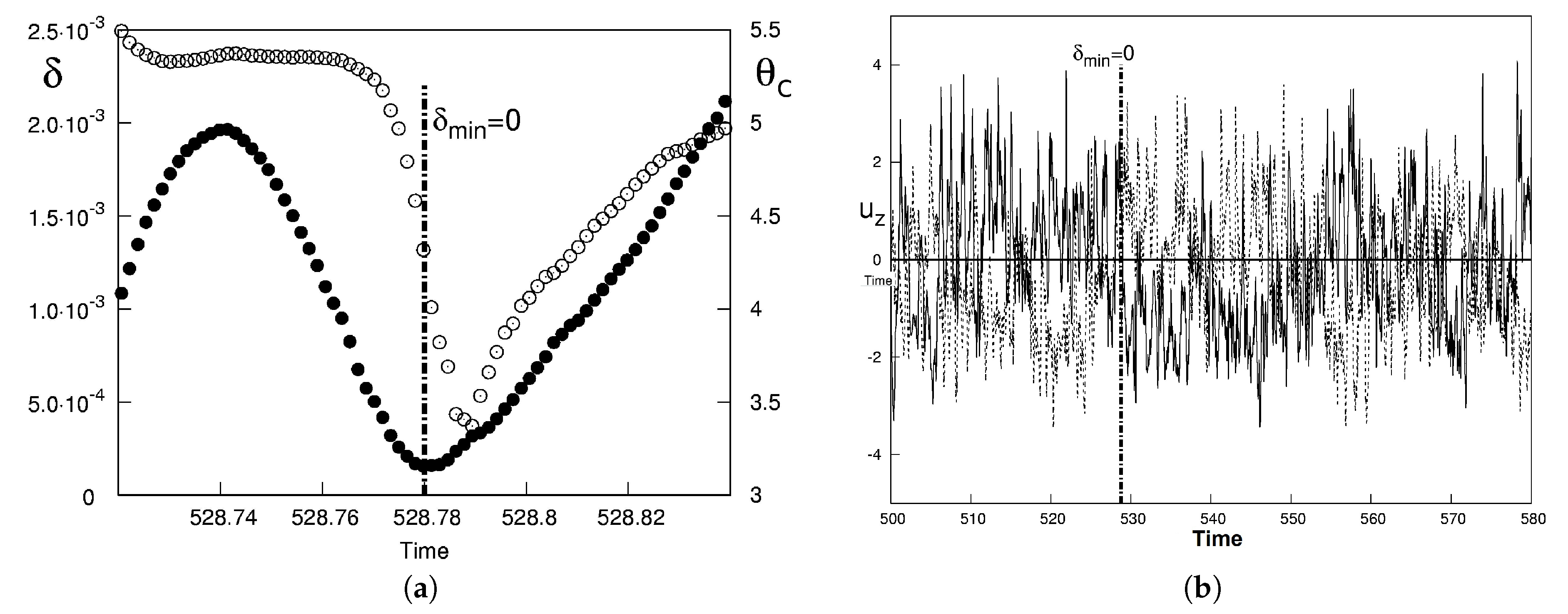
The reorientation of LSC happens several times in the thermal flow forced by bubbles. We analyzed the time evolution of $\delta$ and ${\theta }_c$ in a time interval close to 528.78 (Figure 5). For this time instant, $\delta$ shows a minimum value corresponding to a quick variation of ${\theta }_c$. This means that the fluctuation of the temperature vanishing and simultaneously the LSC is reoriented. Another proof of this behavior is provided by the time evolution of the flow axial velocity recorded in two symmetric positions (probes 3 and 7): its sign changes at the instant for which $\delta$ shows a minimum in connection with the sharp variation of ${\theta }_c$.

The presence of large-scale structures and their reorientation it is very clear if we observe the flow axial velocity plotted in the horizontal section of the cylindrical domain at $z=0.5$ (Figure 6). In the same figure, the orientation of the LCS is reported at time 521.8 and 530. The presence of the large-scale and its orientation suggest a strong relation between the effects of the bubbles and the bulk dynamics of the thermal flow at high Rayleigh numbers without bubbles.

The bubble distribution is highly inhomogeneous (Figure 2) showing clustering and preferential sampling of the up-flow region (Figure 2b) before the reversal involving a random re-mixing process of the bubbles. This phenomenon is confirmed by the strong variation of the Stokes number related to the growing and shrinking process of each bubble as it shown in Figure 7. In the same figure, the volume fraction has a small fluctuation with an averaged value of 0.2.

3.3. Description of the Flow Coherent Structures

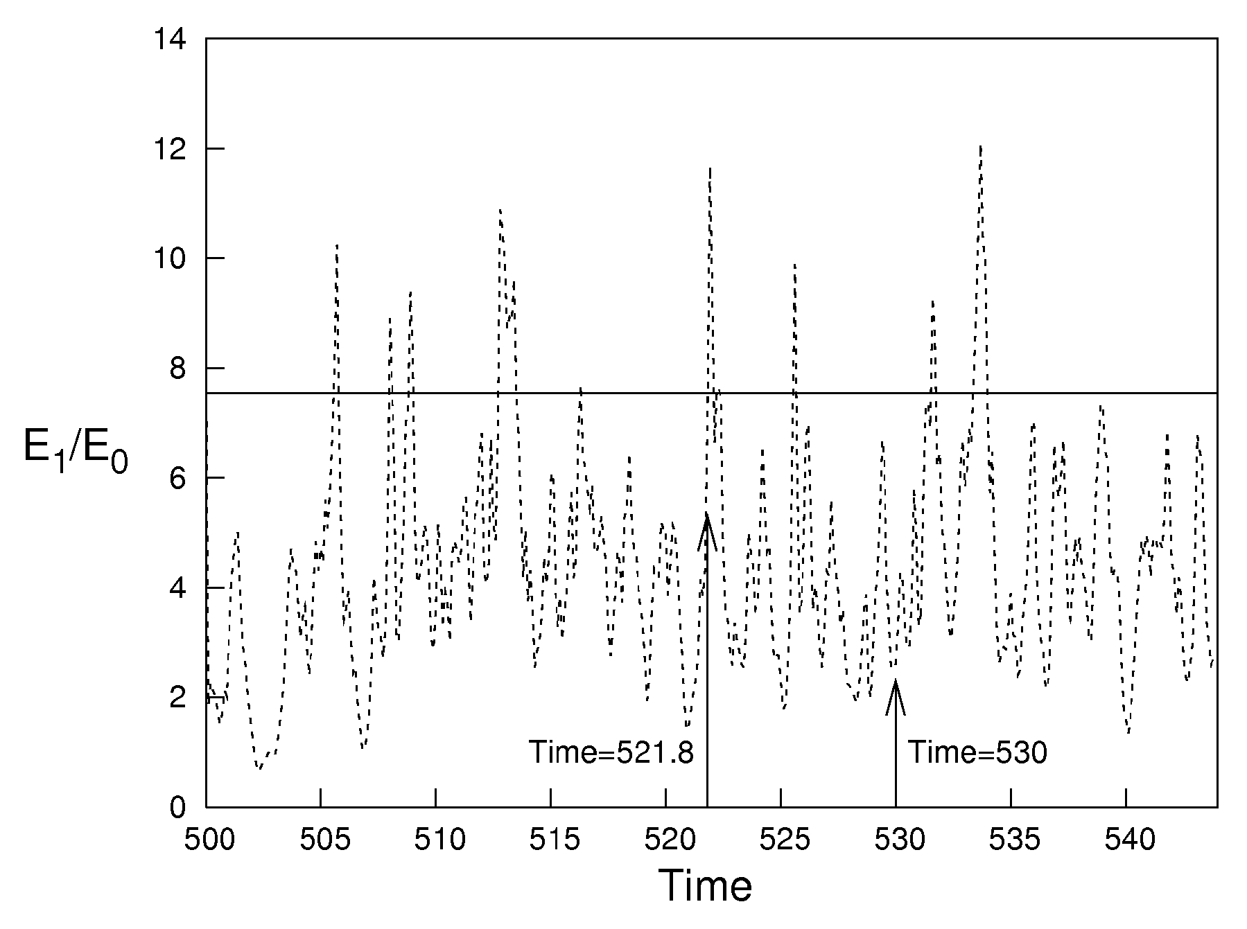
A quantitative way of characterizing the mean flow is determining its energy content: by performing a Fourier transform of the velocity field, its spectrum of n azimuthal modes can be obtained as well as their energy contents; namely, if $\mathbf{u}(\theta ,r,z)$ is the velocity field, its FFT in the azimuthal direction return the matrix $\mathsf{û}(n,r,z)$, where n the azimuthal wavenumber; the azimuthal energy modes are then obtained by integrating $\mathsf{û}(n,r,z){\mathsf{û}}^{*}(n,r,z)$ in r and z, for each wavenumber n, ${\mathsf{û}}^{*}$ being the complex conjugate of û. This decomposition is particularly significant since the $n=0$ mode corresponds to the axial symmetric toroidal structures, the $n=1$ mode contains the energy of the large-scale structures spanning the cell, and the $n\ge 2$ mode are the structures with $n-fold$ azimuthal symmetry.

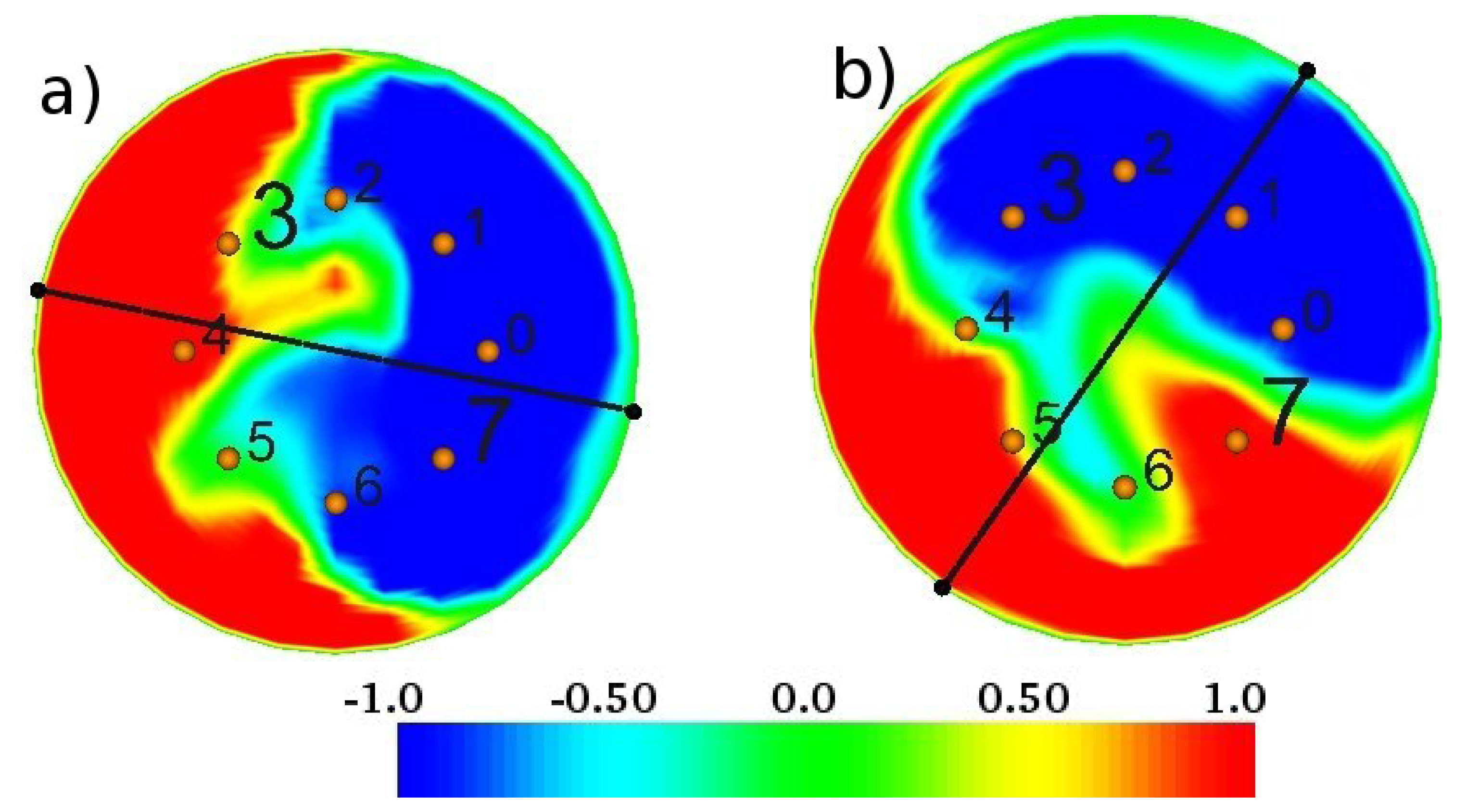
In Figure 8 time history of the ratio between the first and zero mode azimuthal energy: solid line indicates the no bubble flow whereas the dashed line refers to the two-way coupling case. The first mode has higher amount of energy respect to the zero mode only for the flow without bubbles. On the contrary, the dispersion of bubbles makes the amount of energy $E_1$ and $E_0$ comparable at every instant of time in the other case. This means that the large-scale is characterized by a big roll filling the whole domain that temporarily in time switches to structures characterized by a roll coexisting with an axisymmetric vortex. For instance, the flow exhibits these two flow structures at the time 530 when the $E_1/E_0\simeq 2.5$ (Figure 9). The vertical plane crossing the axis at azimuthal position ${\theta }_c$ keep the vortex filling the whole domain: that corresponds to the first mode. Instead, the vertical plane Instead, the vertical plane crossing axis at azimuthal position ${\theta }_c+\pi /4$ keeps the axisymmetric vortex, and that corresponds to the zero mode.

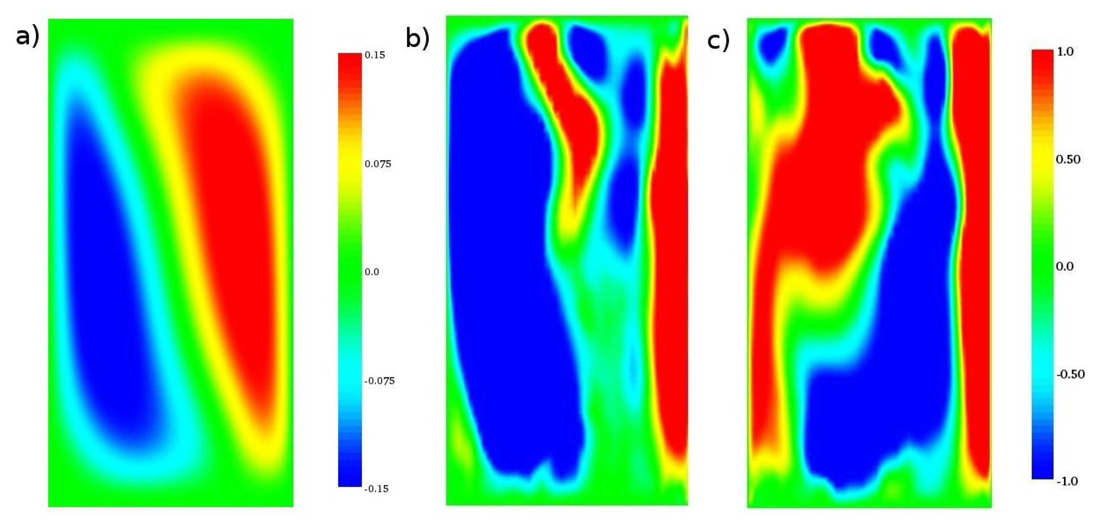
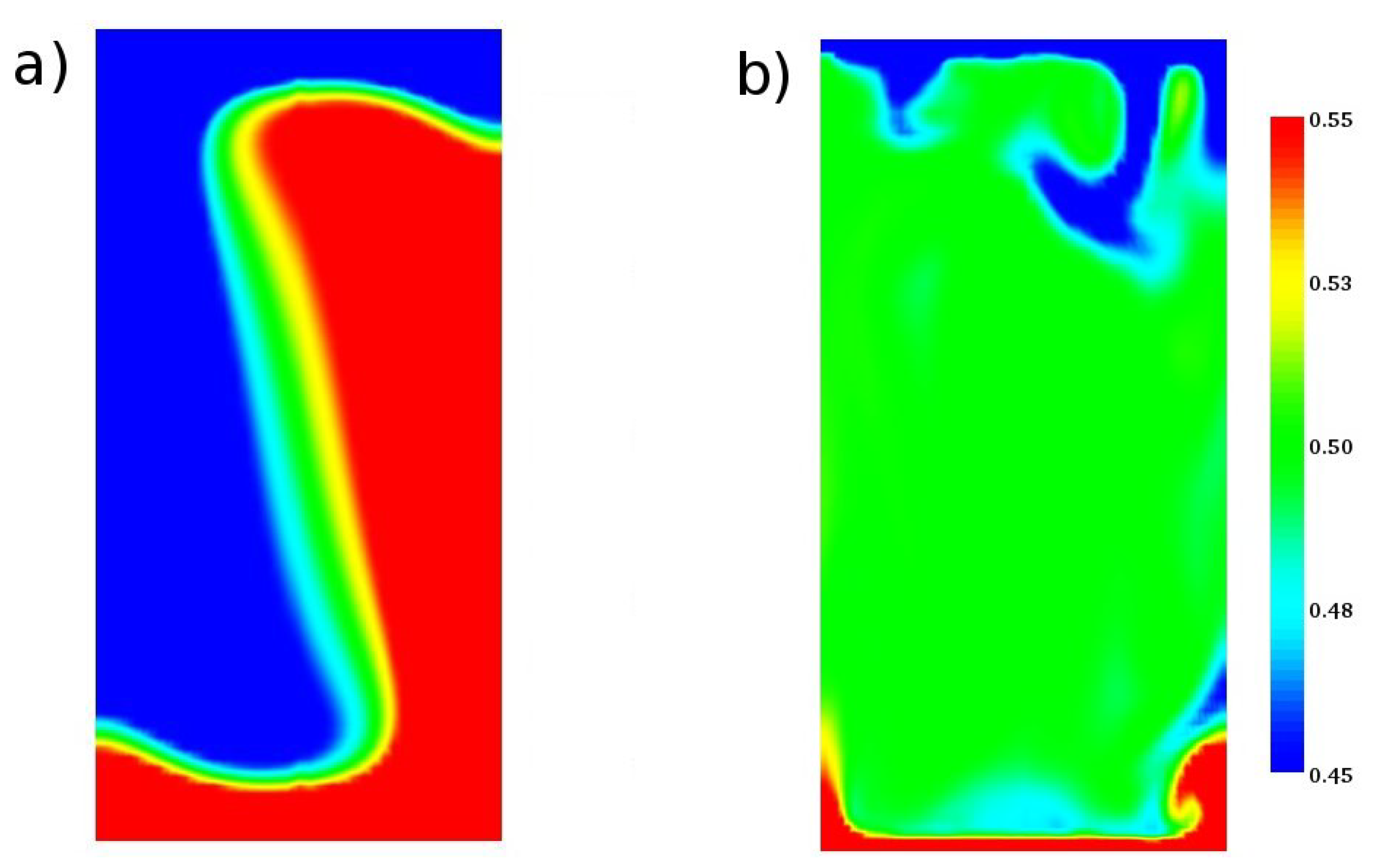
In addition to the effect of the bubbles on the velocity field, the temperature field also deeply changes in the force of the moving bubbles, as shown in Figure 10. In the case of stationary thermal flow without bubble (Figure 10a), the thermal field shows a fluctuation of the temperature in the azimuthal direction that decreases with the two-way coupling because of its re-mixing. Moreover, the bubbles generate elongated structures attached to the upper plate commonly called “thermal plume”. These plumes are like emissions of hot (cold) fluid from bottom (top) thermal boundary layers and are carried by their buoyancy. This observation is another aspect concerning the connection of the thermal flow at high Rayleigh numbers with the effects due to the bubbles dispersed in a stationary convective flow.

4. Conclusions

The Multi-phase Rayleigh–Bénard convection was investigated in a confined slender cylindrical domain. At moderate Rayleigh number, the single-phase flow shows a stationary state of the large-scale circulation characterized by a single roll filling the domain. When this coherent structure becomes unsteady, it causes the nucleation of vapor bubbles.

The time history of the Nusselt number shows a Gaussian distribution where the rare tail events connected with the bubble dynamics overlap with the average main stream flow.

This phenomenon apparently disagrees with the instantaneous clustering of the bubbles that preferentially place themselves in the ascending flow. Those effects coexist, since the LSC changes its azimuthal position in time, so sweeping the whole section area trough quasi-stationary azimuthal configurations.

The numerical approach could detect the wind reversal induced by the bubble dispersion showing that, by considering an averaged dynamics, the Nusselt number is randomly affected by the bubbles, even though it shows instantaneous preferential interaction with the flow structure populating the cylindrical domain.