Revisiting Two Simulation-Based Reliability Approaches for Coastal and Structural Engineering Applications

Featured Application

Normality polynomials can be used to compute reliabilities for coastal and structural engineering applications, including the assessment of uncertainty in the estimated reliability index. Additionally, multi-linear regression can be applied to the simulated results to determine design points and sensitivity factors. These applications can be potentially extended to different engineering (or other) fields and to system reliability (e.g., for reinforced concrete frame buildings).

Abstract

The normality polynomial and multi-linear regression approaches are revisited for estimating the reliability index, its precision, and other reliability-related values for coastal and structural engineering applications. In previous studies, neither the error in the reliability estimation is mathematically defined nor the adequacy of varying the tolerance is investigated. This is addressed in the present study. First, sets of given numbers of Monte Carlo simulations are obtained for three limit state functions and probabilities of failure are computed. Then, the normality polynomial approach is applied to each set and mean errors in estimating the reliability index are obtained, together with its associated uncertainty; this is defined mathematically. The data is also used to derive design points and sensitivity factors by multi-linear regression analysis for given tolerances. Results indicate that power laws define the mean error of the reliability index and its standard deviation as a function of the number of simulations for the normality polynomial approach. Results also indicate that the multi-linear regression approach accurately predicts reliability-related values if enough simulations are performed for a given tolerance. It is concluded that the revisited approaches are a valuable option to compute reliability-associated values with reduced simulations, by accepting a quantitative precision level.

1. Introduction

Simulations are often used to estimate the probability of failure of structural elements and systems because they are a very versatile option which is not restricted by complex and implicit limit state functions (LSF), the use of sophisticated methods (e.g., finite element method), and/or highly non-linear structural behavior. However, millions of crude Monte Carlo simulations (MCS) could be required to adequately estimate structural probabilities of failure, which may not be feasible; also, the results could differ from a set of simulations to another. To cope with this issue, modified versions of the crude simulation approach, surrogate modeling, subset simulation, and other techniques have emerged and been used in the last decades not only for structural engineering but also in other fields. To mention only a few studies which employ some of these techniques, optimization using surrogate modeling, reliability analysis of deteriorating structural systems and the reliability assessment of a structure affected by chloride attack are reported in the studies by [1,2,3], respectively. Importance sampling has also been used to estimate the system reliability of deteriorating pipelines [4]. Other kind of approaches are also reported in the literature to compute reliabilities [5]. The different reliability methods can be applied not only to different fields in structural and geotechnical engineering, as for the case of sudden column removal in reinforced concrete buildings and rockfall protection structures [6,7,8], but also to many other research and engineering fields, for instance to artic oil and gas facilities [9] and to coastal engineering applications [10]. This last case is used in the present study to show the applicability of two revisited methods to obtain the reliability of coastal structures.

Other simulation-based reliability methods have not been given so much attention. In this study a couple of these alternatives are revisited to inspect their feasibility and adequacy to estimate reliability indices. One of them employs polynomial transformations of a nonnormal variable to a normal one by fitting simulated data with fractile constraints and can be referred to as normality polynomial approach [11]. The second approach was developed to derive the design point and sensitivity factors (in the FORM, first order reliability method, perspective) from simulated data [12] and it is referred to as the multi-linear regression approach in this study. A similar approach to the normality polynomial method was previously developed by Hong and Lind [13] and named normal polynomial approach (note that the names are slightly different); unlike the normality polynomial approach, the normal polynomial approach has been paid much more attention (judging by number of citations), even very recently (e.g., [14]). Both methods are based on the fact [15,16] that a fractile of a random variable can be expressed as polynomial of a fractile of a standard normal variable (normal polynomial), and that a fractile of a standard normal variable can be expressed as a polynomial of a fractile of a random variable (normality polynomial). Although the normal polynomial approach [13] is not considered in the present study (we prefer to focus in the less explored alternative), the findings here could be extended to do so.

To inspect the adequacy of the normality polynomial approach and the multi-linear regression approach (the methods revisited in the present study), three LSFs are considered. One is based on a very simple classical case; other one is based on a structural application from a previous study and the last one is related to the reliability of a coastal structure. Extensive simulations are performed to estimate the error level by using the normality polynomial approach and its associated uncertainty; neither of these was thoroughly carried out in previous studies, nor the application to coastal engineering. The design point and sensitivity factors (also the reliability index) obtained from simulated data are compared with those obtained from FORM; they are derived from a multi-linear regression of the simulated data. It is worth to mention that these methods, and others developed in the 1990s, used to state that a large number of simulations were not feasible; nevertheless, the computer power has increased substantially in the last decades, and the limitations of those days may not be as restrictive as before and thus the applicability could be currently extended. Furthermore, the commercial software available nowadays for engineering applications normally includes amenable built-in functions for linear and multi-linear regression analysis which simplifies the programming.

The main objective of this study is to define the error statistics in the reliability index by using normality polynomials and to reassess the feasibility and adequacy of this method and the multi-linear regression approach for estimating the reliability of structural and coastal engineering systems including the determination of sensitivity factors.

This study is of significance to the coastal and structural engineering fields because the number of simulations required to compute reliabilities can be reduced by accepting defined error levels when using normality polynomials, which was not established in previous studies. This is possible because the error in the estimation of the reliability index is mathematically defined as a function of the number of simulations for the cases investigated. Additionally, other contribution is the use of multi-linear regression applied to simulated results as a mean to determine sensitivity factors, design points and the probability of failure; not only a slightly modified (improved) version of the multi-linear regression approach but also the number of simulations and tolerances required to achieve adequate results are provided for guidance.

2. Methods Revisited

2.1. Normality Polynomial

In this section the normality polynomial proposed in [11] is described. The mathematical form is given by

$$z_p={\displaystyle \sum }_{j=0}^r{a}_j{\left(y_p\right)}^j$$

(1)

where z_p denotes p-fractile of a standard normal variable Z with probability density function (PDF), Φ(z), and cumulative distribution function (CDF), Φ(z); y_p denotes p-fractile of a random variable Y with PDF, f_Y(y), and CDF, F_Y(y); a_j, j = 1, 2, …, r, are the coefficients of a rth-order polynomial determined by fractile fitting. The fractile fitting is based on considering the following fractile constraints from a set of independent random observations of Y (i.e., y₁, y₂, … y_i, … y_n) arranged in ascending order

$$\left(y_i, F\left(y_i\right)\right)= \left(y_i, \frac{i}{n+1}\right), i=1, 2, \dots , n$$

(2)

These fractile constraints can be mapped into a normal space by using

$$z_i={\mathsf{\Phi }}^{-1}\left(F\left(y_i\right)\right), i=1, 2, \dots , n$$

(3)

where Φ⁻¹(•) denotes the inverse of the standardized normal distribution function. The rth-order polynomial (Equation (1)) with r + 1 < n is used to model the distribution of the transformed random variable Y. By considering the constraints in Equation (2), the coefficients a_j in Equation (1) can be determined using the least square method by minimizing the error ε_fit given by

$${\epsilon }_{fit}={\displaystyle \sum }_{j=1}^m{\left(z_j-{\displaystyle \sum }_{i=0}^r{a}_i{\left(y_j\right)}^i\right)}^2$$

(4)

where m is the number of constraints. The probability P (Y ≤ y₀) is given by the CDF, i.e., F(y₀), and can be computed with

$$F\left(y_0\right)=\mathsf{\Phi }\left(z_p\right)$$

(5)

where z_p is obtained by substituting y₀ instead of y_p in Equation (1). If Y is the resulting random variable of the LSF, the probability of failure, p_f, is

$$p_f=F\left(0\right)=\mathsf{\Phi }\left(a_0\right)$$

(6)

and the reliability index is [17]

$$\beta =-{\mathsf{\Phi }}^{-1}\left(p_f\right)$$

(7)

From Equation (7), it can be inferred that the reliability index can be readily obtained once the coefficients a_j are determined (i.e., β = −a₀). This is so, because a₀ has a similar meaning to the so-called generalized reliability index [11]. It is noted that the roots of the polynomial are not required [11] (unlike in the method in [13]). In the applications shown later, a third-order normality polynomial is used [11].

It is pointed out that although the mathematical background of the normality polynomials is not thoroughly described here, it is based on sound grounds [11], like the advance theory of statistics [15,16] and the fact that fractile constraints hold by a combinatorial argument [18,19].

Before going to the applications, the second revisited approach in this study is described in the following section.

2.2. Design Point and Sensitivity Factors from Simulations

The obtaining of the design point and sensitivity factors (from the FORM standpoint) based on a previous study [12] is described herein. The basic idea is that simulated data close to the limit state surface (within a prescribed tolerance, e) can be retrieved, as well as their associated sampled values for each or the random variables given by the LSF (input values combinations considered as a point in the hyperspace), and a multi-linear regression is performed to approximate the linearized limit state surface at the design point. Before the multi-linear regression is performed to fit the hyperplane, the considered points are mapped into a standard normal space. Such hyperplane is an approximation of the LSF, g, and is used to assess the design point and sensitivity factors. The mathematical formulation is given below.

A set of n independent random variables is denoted by X = (x₁, x₂, …, x_n). X^j defines the j-th randomly generated value of X. For a given number of crude Monte Carlo simulations, n_sim, X_js which satisfy the criterion below (slightly changed from the original formulation in [12]) are selected

$$\left|0-\mathrm{g}\left({\mathit{X}}^k\right)\right|<e_l$$

(8)

where X^k in the LSF is included to emphasize that it is a function of a set of random variables. Hong and Nessim [12] used e = 0.05 (i.e., 5%) in their study (instead of e_l in Equation (8) and defined below). However, it was noticed that this value could be inadequate depending on the units and magnitude of the considered random variables. Therefore, the distance between zero and the smallest simulated value of g in absolute terms (l_low) is used to set the tolerance as the fraction given by l_low multiplied by e (i.e., e_l = e × l_low is used instead of e in Equation (8)). The selected values of X^k based on the described criterion are then mapped into a standard normal space [17] using

$$\mathit{Z}=\left[z_1,z_2,\dots ,z_n\right]=\left[{\mathsf{\Phi }}^{-1}\left(F_1\left(x_1\right)\right),{\mathsf{\Phi }}^{-1}\left(F_2\left(x_2\right)\right),\dots ,{\mathsf{\Phi }}^{-1}\left(F_n\left(x_n\right)\right)\right]$$

(9)

where Z is the image of X in standard normal space, Φ is the normal standard CDF and F_i, I = 1, 2, …, n, are the CDFs of the random variables x_i. In the standard normal space, a linear function is fitted to the set of selected points using multi-linear regression. Such linear function is given by

$${{\displaystyle \sum }}_{i=1}^n{b}_i{z}_i+c=0$$

(10)

where b_i and c are constants to be determined in the multi-linear regression analysis. The resulting linear regression equation is to be used in the same sense as the FORM [17] to estimate the design point and sensitivity factors. The latter are denoted by α_i, i = 1, 2, …, n, and given by the gradient vector of Equation (10) as indicated below

$${\alpha }_i=\raisebox{1ex}{$-b_i$}\!\left/ \!\raisebox{-1ex}{$\sqrt{{{\displaystyle \sum }}_{i=1}^n{b}_i^2}$}\right.$$

(11)

Note that the reliability index can also be estimated as the smallest distance between the linear surface and the origin as

$$\beta =\raisebox{1ex}{$c$}\!\left/ \!\raisebox{-1ex}{$\sqrt{{{\displaystyle \sum }}_{i=1}^n{b}_i^2}$}\right.$$

(12)

As regards the design point (in the normal space) it is given by

$$z_{id}={\alpha }_i\beta$$

(13)

The design point in the original space can now be determined with the inverse transformation of z_id, as

$$x_{id}=F_i^{-1}\left(\mathsf{\Phi }\left(z_{id}\right)\right)$$

(14)

The subscript i in Equations (11)–(14) is associated to the random variable x_i. The inverse transformation in Equation (14) is dependent on the PDF of x_id and, in the case of the Longuet-Higgins distribution [20] used for the coastal engineering example, the inverse transformations of z_id requires of a numerical approach to be determined.

The formulation in this section, and the one in the previous section, are to be applied to three case studies in the following section to evaluate their adequacy for structural and coastal engineering, and to assess their deviation with respect to the exact reliability index.

3. Applications and Results

3.1. A Classical Limit State Funtion

The two approaches described in the previous section are applied here to the simplest classical LSF

$$g=R-L$$

(15)

where R and L can be considered, in a broad sense, as random variables for the capacity and demand of a system element. For the sake of simplicity and illustration purposes, units are skipped and both random variables are assumed independent and characterized with lognormal distributions, with mean values and standard deviations m_R = 10, m_L = 5.6, σ_R = 1, and σ_L = 0.75 for the capacity and demand, respectively. These values are arbitrary, except by the fact that they lead to a reliability index equal to practically 3.5, which is a common reference for code calibration and that can be computed with the following expression [21,22]

$${\beta }_{RE}=\frac{\left(ln m_R-\frac{1}{2}\ln \left(1+{\upsilon }_R^2\right)\right)-\left(ln m_L-\frac{1}{2}\ln \left(1+{\upsilon }_L^2\right)\right)}{\sqrt{\ln \left(1+{\upsilon }_R^2\right)+\ln \left(1+{\upsilon }_L^2\right)}}\approx \frac{\ln m_R-\ln m_L}{\sqrt{{\upsilon }_R^2+{\upsilon }_L^2}}$$

(16)

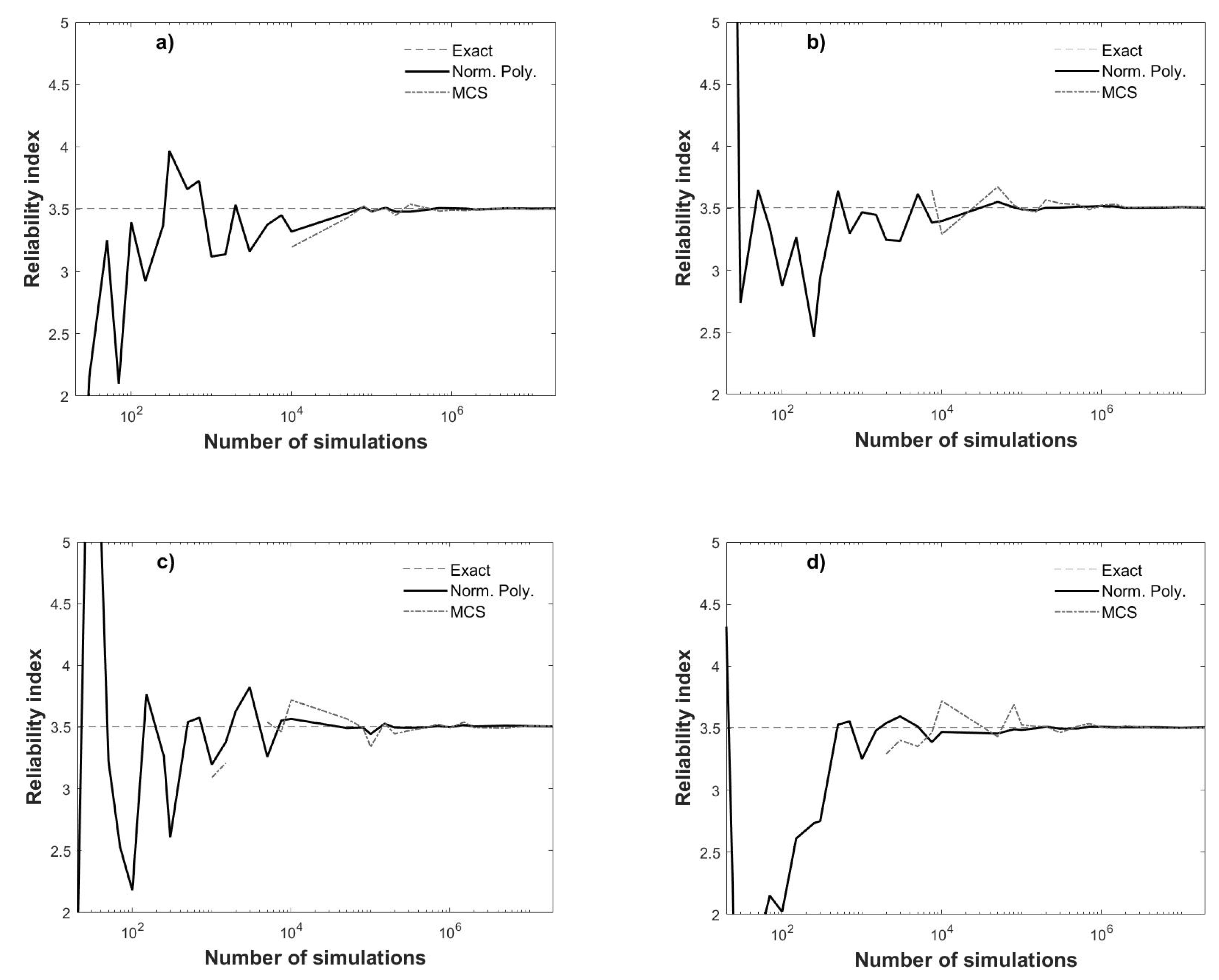
where ν_R and ν_L are the coefficients of variation of R and L, respectively. This reliability index is shown in Figure 1a (dashed line), as a reference to inspect how close are the βs obtained by crude Monte Carlo simulations as a function of the number of simulations (shown in logarithmic scale in the horizontal axis from 2 × 10¹ to 2 × 10⁷) to the exact value. The reliability index for Equation (15) using Monte Carlo simulations (dashed-dotted line in Figure 1a) is obtained by plugging into Equation (7) the following probability of failure

$$p_f=\raisebox{1ex}{$n_{fail}$}\!\left/ \!\raisebox{-1ex}{$n_{sim}$}\right.$$

(17)

which is simply the ratio of number of failures, n_fail, to the total number of simulations. The latter (i.e., n_sim) is also the number of fractile constraints when the reliability index is computed with the normality polynomial approach, also depicted in Figure 1a (solid line).

Additional runs are shown in Figure 1b–d, which indicate that the results are different and dependent on the generated random numbers of each run, but they stabilize if enough simulations are performed or enough fractile constraints are used. Other observations from Figure 1 include that β cannot always be computed with the Monte Carlo simulations (MCS) (not a single failure is obtained), while the opposite occurs when using normality polynomials, although significant deviations are observed for a limited number of simulations, that the fitted normality polynomials tends to deviate less from the exact reliability index for fewer n_sim, and that such error in the precision may not be large for a relative small n_sim, (e.g., 1 × 10³).

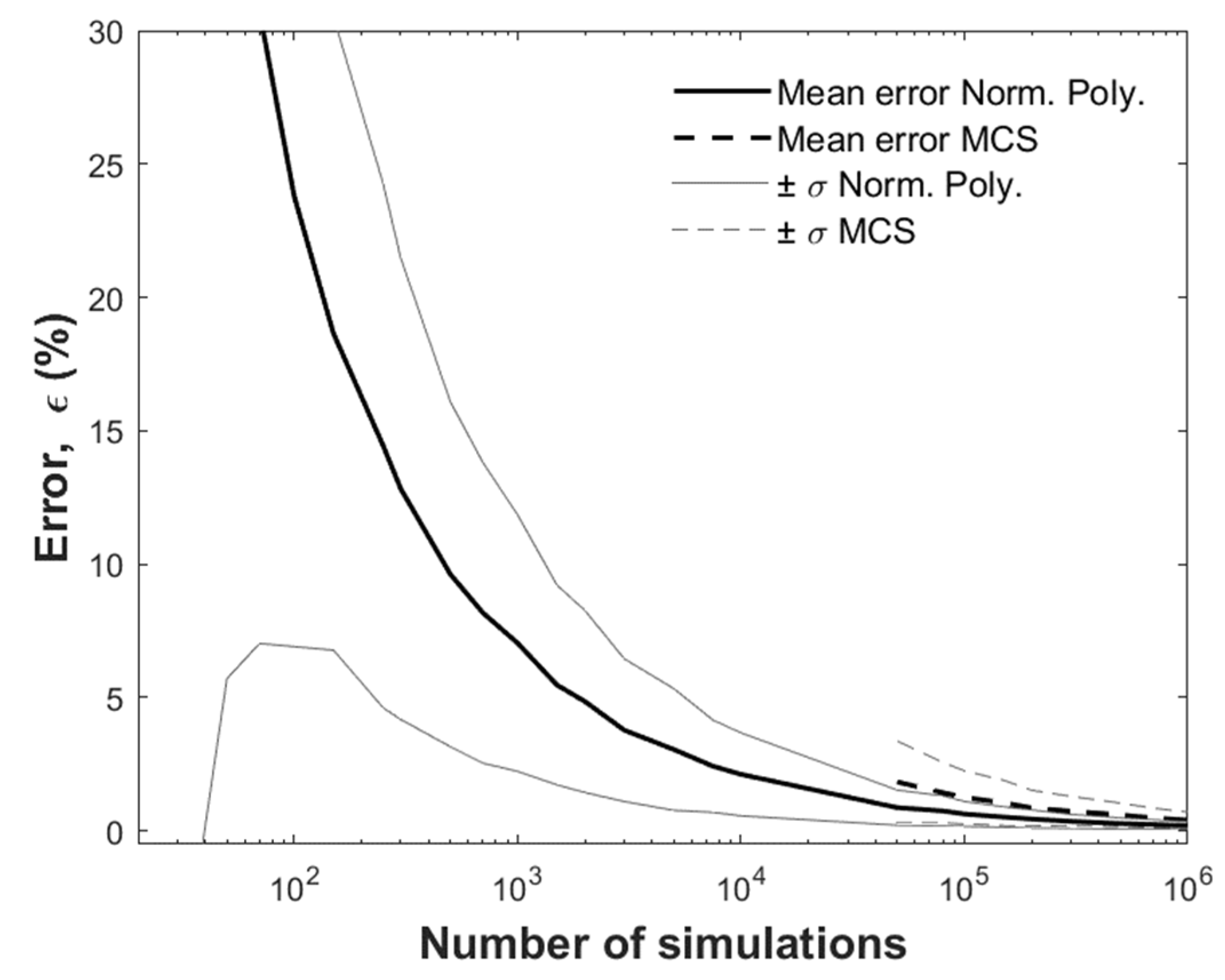
To quantitatively inspect these deviations, β_RE is to be used as benchmark to assess the exactness of the used methods (i.e., normality polynomials and MCS) in terms of the relative percentual error given by

$$\epsilon =\left|\frac{{\beta }_{bench}-{\beta }_{oth}}{{\beta }_{bench}}\right|\times 100$$

(18)

where β_bench denotes the reliability index considered as benchmark and β_oth is the reliability index computed with any other method. A total of 1000 runs are performed for each n_sim, and ε is computed for each of the runs. Then, the mean values of the error and their uncertainties (the unbiased standard deviation) are computed and plotted for the whole range of n_sim in Figure 2 (solid lines and dashed lines for normality polynomial and MCS mean errors, respectively), where the mean errors ± one standard deviation are also depicted in grey lines.

Figure 2 shows that is not always possible to compute the statistics for the MCS; this happens when not a single failure is reported in one or more of the 1000 runs for a given n_sim (at least 5 × 10⁴ are necessary). This is not a problem when using the fitted polynomials. Additionally, the MCS approach always tend to larger mean errors and standard deviations for a decreasing number of simulations. This makes the normality polynomial approach more adequate for estimating the reliability indices; however, for few simulations the errors are too large. Nevertheless, the designer could decide which precision level (quantitatively) is willing to accept using information like the one in Figure 2 as an aid (and reduce the number of required simulations as a function of such an accepted error).

If desired, the curves in Figure 2 could be casted as a mathematical expression. For instance, the following power equations fit very well the mean (μ_ε) and standard deviation (σ_ε) of the error in Figure 2 (by fitting from 2.5 × 10² simulations and over)

$${\mu }_{\epsilon }=257.2\times n_{sim}^{-0.5244}$$

(19)

$${\sigma }_{\epsilon }=157.3\times n_{sim}^{-0.5068}$$

(20)

If the power in Equations (19) and (20) is assumed as −0.5 in both expressions, the coefficient of variation of the error is ν_ε ≈ 150/250 ≈ 0.6, i.e., it is constant and roughly independent of the number of simulations; the actual ν_ε obtained from the 1000 runs does exhibit such a roughly constant behavior for this case, except that it is ≈0.7 (difference related to the actual different powers in Equations (19) and (20)). Power equations like Equations (19) and (20) can be linearized by taking logarithms on both sides. Therefore, if the involved variables are transformed into the logarithmic space, a linear fitting can be performed. In this study, we simply used a built-in function in the commercial software for the fitting.

Coefficients for the fitted normality polynomial in Figure 1a are shown in

Table 1. Coefficients of the fitted normality polynomials.

	Classic LSF, Equation (15)
nsim	a0	a1	a2	a3	a4
1 × 103	−3.1193	3.9078	3.6571	−1.9371	----
1 × 104	−3.3195	4.9672	1.8106	−0.9905	----
1 × 105	−3.4813	5.8709	0.2415	−0.1324	----
	Structural LSF, Equation (21)  rV/D= 0.4
nsim	a0	a1	a2	a3	a4
1 × 103	−3.0950	6.3170 × 10−07	3.8257 × 10−14	−3.2619 × 10−21	----
1 × 104	−3.2923	7.3372 × 10−07	2.1457 × 10−14	−2.3097 × 10−21	----
1 × 105	−3.3341	7.8972 × 10−07	5.2658 × 10−15	−1.0534 × 10−21	----
	Structural LSF, Equation (21)  rV/D = 0.4 4th-order
nsim	a0	a1	a2	a3	a4
1 × 103	−2.8726	1.7464 × 10−07	2.7997 × 10−13	−5.0461 × 10−20	3.1134 × 10−27
1 × 104	−3.2802	6.7401 × 10−07	6.0193 × 10−14	−1.0616 × 10−20	5.7321 × 10−28
1 × 105	−3.2799	7.1276 × 10−07	3.6215 × 10−14	−5.7785 × 10−21	2.4322 × 10−28

(upper set of values) for selected values of n_sim. The computing of these coefficients is based on minimizing the error in Equation (4) and was implemented in the coded program by using a built-in function of the programming language employed (MATLAB). As mentioned before, the coefficients a₀ can be linked to the generalized reliability index. Coefficients for results in Figure 1b–d (or those associated to Figure 2) were computed but not shown for brevity.

As regards the reliability index, design point and sensitivity factors derived from the simulations (i.e., those obtained with Equations (11), (12), and (14)), they are compared with those obtained by applying the FORM to Equation (15). They are summarized in

Table 2. Design point, β and α_i by using multi-linear regression and first order reliability method (FORM).

		Design Point		Sensitivity Factors
nsim	β	xR	xL	αR	αL
1 × 104	----	----	----	----	----
5 × 104	----	----	----	----	----
1 × 105	3.5055	8.0699	8.0699	−0.5990	0.8007
2 × 105	3.5055	8.0699	8.0699	−0.5990	0.8007
1 × 106	3.5055	8.0699	8.0699	−0.5990	0.8007
FORM	3.5055	8.0670	8.0670	−0.5990	0.8007

for selected values of n_sim.

Results listed in Table 2 indicate that when the points obtained by applying the criterion in Equation (8) were enough to successfully perform a multi-linear regression (also with a built-in function, as in the case of the normality polynomial fitting), β did not deviate from the exact value, but marginally, just like the reliability index obtained with FORM. However, a relatively large n_sim was required, usually at least 1 × 10⁵ simulations (by inspecting all the 1000 × n_sim cases used to derived Figure 2); this depends on each run (implicitly the generated random numbers in each simulation), and sometimes less than 1 × 10⁵ simulations are required. For the considered runs, 2 × 10⁵ simulations seem to guarantee the obtaining of the values reported in Table 2. In any case, when the muti-linear regression is successfully performed, the results are quite adequate and invariant for increasing number of simulations; this is also the case for the coefficients of the regression (i.e., they remain independent of n_sim), which are c = 0.5837, b₁ = 0.0998, and b₂ = −0.1333.

If the tolerance e_l in Equation (8) is increased, the minimum number of required simulations can be decreased. For instance, if e = 0.25 were used (instead of the actual used e = 0.05), 5 × 10⁴ simulations would be enough for a successful multi-linear regression. Moreover, the design point, sensitivity factors and reliability index would be the same as those reported in Table 2. The opposite would occur if e = 0.005 were used (instead of the actual used e = 0.05), i.e., a much larger number of simulations would be required to determine the reliability parameters from the regression.

Therefore, this approach based on multi-linear regression can be quite an adequate alternative by itself to compute β, conditioned on the feasibility of performing enough simulations, the number of which can be decreased by using a large e; with the additional advantage that the design point and sensitivity factors can also be determined.

In the following section a more realistic LSF for a structural application is used to further investigate the revisited methods.

3.2. Reliability of Reinforced Concrete Beam under Flexure Moment

In this section the approaches described before are applied to a reinforced concrete beam (RCB) subjected to flexure moment. The example is the same investigated in a previous study [23] but focused only in one design code [24] and three ratios of the mean live to the mean dead load effect for the beam. The rectangular beam section information, LSF, and statistics are succinctly reproduced below. The LSF is

$$g_{ACI}=B{A}_s{f}_{y}d\left(1-0.59\frac{A_s{f}_y}{f_c^{\prime }bd}\right)-D-V$$

(21)

where B is the modeling error, f’_c is the concrete compressive strength, A_s is the reinforcement steel area, f_y is the yielding stress of the reinforcement steel, b is the section width, h is the effective depth, and D and V are the dead load and live load effect, respectively (flexure moment). The information of all the independent variables in Equation (21) is summarized in

Table 3. Random variables for the limit state functions (LSF) of the reinforced concrete beam (RCB) considered.

Random Variable	Mean	coeff. of var.	PDF
B	1.01	0.06	Normal
f’c (MPa)	31.6	0.145	Normal
fy (MPa)	474	0.05	Lognormal
b (mm)	303	0.04	Normal
d (mm)	990	0.04	Normal
D (kN·m)	*	0.05	Normal
V(kN·m)	*	0.18	Gumbel

* denotes that these values are not determined until a r_V/D value is selected and used together with Equation (22).

. A_s is assumed deterministic and equal to 3000 mm². The PDFs of the random variables in Table 3 are based on previous literature, which in turn reflects results from experimental projects, field information, observed phenomena, and even the engineers experience to characterized these variables properly, since such PDFs have a direct impact in the computed reliabilities, code calibration tasks, and ultimately in the safety of real structures. More details can be found in [23] and the references therein.

Mean values of D and V are not defined in Table 3, but they are derived by considering given mean live load effect (m_V) to mean dead load effect (m_D) ratios (r_V/D = 0.4, 1.0 and 2.0 are used in this study) and the assumption that the RCB just meets the code requirement; thus, the following expression is used to determine the mean values.

$$1.2m_D+1.6m_V=\varphi A_s{m}_{f_y}\left(m_d-0.59\frac{A_s{m}_{f_y}}{m_{f_c^{\prime }}{m}_b}\right)$$

(22)

where m denotes the mean values of the variables in the corresponding subscripts, and Φ = 0.9.

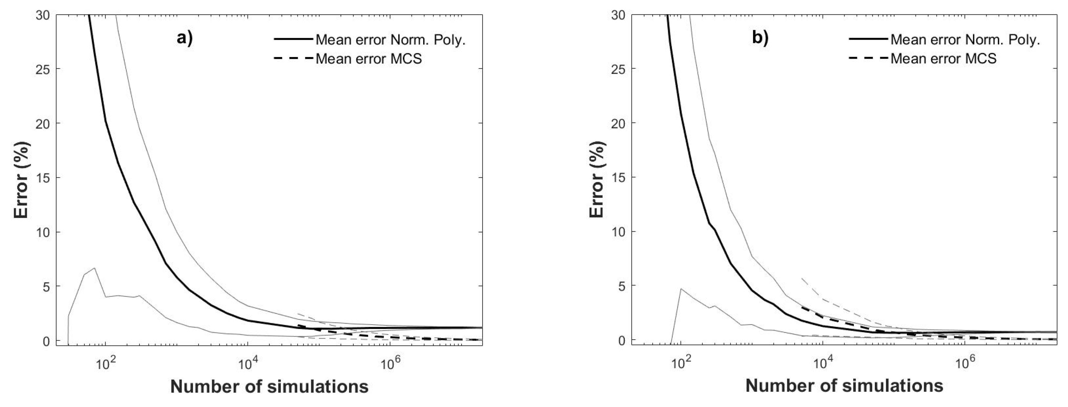
Using the previous information, the normality polynomial approach is applied to Equation (21) and the results are shown in Figure 3 and Figure 4. These figures are analogous to Figure 1 and Figure 2, except that the reference reliability indices (dashed lines) correspond to the values computed using FORM, that three cases of the ratio r_V/D = m_V/m_D are depicted (the largest βs correspond to r_V/D = 0.4 and the smallest to r_V/D = 2.0, as shown in Figure 3a) and that the error in Figure 4 is shown for r_V/D = 0.4 (Figure 4a) and for r_V/D = 2.0 (Figure 4b), which is computed by considering in Equation (18) β_bench as the average of the 1000 runs for n_sim = 2 × 10⁷ (assumed as the exact value). MCS results are depicted with dashed-doted lines. To perform the MCS, m_D and m_V are defined using Equation (22) and r_V/D as mentioned before. 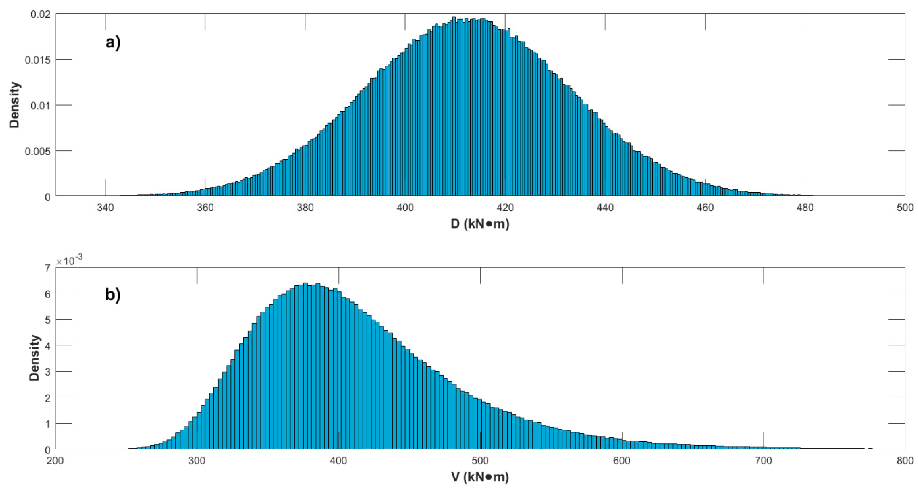Once they are determined, MCS can then be performed to obtain samples of D and V (and all other random variables in Table 3) and the probability of failure as per Equation (17) can be computed. As an example of the simulated bending moments, histograms of D and V are shown in Appendix A (Figure A1) for 1 × 10⁶ MCS and r_V/D = 1.0; it can be observed that the values are comparable in average (because r_V/D = 1.0 is considered), and that histograms for D and V clearly resemble normal and Gumbel distributions, respectively, which is expected given that these variables were sampled from such PDFs.

From Figure 3 and Figure 4 similar conclusions to those drawn from Figure 1 and Figure 2 can be extracted. Some additional observations worth to mention are that n_sim = 1 × 10⁴ seems a reasonable number of simulations for the normality polynomial approach, if a compromise between n_sim and error (in terms of mean and standard deviation) is envisaged, that the fitted polynomials lead to better results than the FORM for increasing n_sim and that larger errors are obtained for smaller r_V/D; this latter aspect could be attributed to a better approximation of the failure surface for larger r_V/D, since the first order approximation to the failure surface by the other method shown in Figure 3 (i.e., the FORM), also deviates more from the exact value for decreasing r_V/D.

By observing Figure 4, it is pointed out once more that error and its uncertainty is less for normality polynomial when decreasing n_sim than for MCS for this case too and, as previously mentioned, is not always possible to estimate the error for MCS for decreasing number of simulations. The error for β obtained with the normality polynomial approach exhibits an asymptotic behavior towards approximately μ_ε = 1% for large n_sim. As before, power laws fit adequately the error and its uncertainty and are defined as

$${\mu }_{\epsilon }=\delta \times n_{sim}^{-\gamma }+1$$

(23)

$${\sigma }_{\epsilon }=\kappa \times n_{sim}^{-\tau }$$

(24)

where δ = 656, 1103, and 1349, γ = 0.7401, 0.8493, and 0.9062, κ = 129.8, 201, and 179.1, τ = 0.4937, 0.5609, and 0.5703 for r_V/D = 0.4, 1.0, and 2.0, respectively. In Equation (23) the constant unity is included to shift the curve upwards to reproduce the asymptotic behavior mentioned; nonetheless, it could be skipped, and the equations will still fairly adequately describe the mean error. The fitting for μ_ε was performed for the whole range of n_sim, while for σ_ε, n_sim from 250 and over was employed. Note that although the range for the fitting could be established based on practical grounds and fitting improvement, in any case the errors and their uncertainties follow a power law; this is the case for the three case studies carried out in this study.

It is noteworthy that the normality polynomial approach leads to comparable μ_ε and σ_ε for Figure 2 and Figure 4, considering that the LSF for the RCB is a more complex (non-linear) function, and that it has much more random variables and several PDFs.

The fitted coefficients of the polynomials for Figure 3 (corresponding to r_V/D = 0.4) and selected n_sim are listed in Table 1 (middle set of values). If normality polynomials of order higher than 3 are used, no further accuracy is gained (or even higher inaccuracies could be obtained; [11]). This is confirmed by carrying out a single case for r_V/D = 0.4 using a 4th-order polynomial, since the results are comparable to those of the 3rd-order polynomial case (Table 1, lower set of values). Note that the order of the coefficients of the normality polynomials for the RCB problem can be very small (compared to the classical LSF problem and to a coastal engineering application shown later); this could be due to the units employed, and should not be understood as if the order of the polynomial could be decreased, whereas obtaining comparable precision, because the use of at least third-order normality polynomials was illustrated and found adequate in [11].

To end this section, the results of using the multi-linear regression approach for the LSF defined in Equation (21) are listed in

Table 4. Design point, β and α_i by using multi-linear regression and FORM for the RCB.

		Design Point/(Sensitivity Factors)
nsim	β	xB/(αB)	xfy/(αfy)	xf’c/(αf’c)	xD/(αD)	xV/(αV)	xb/(αb)	xd/(αd)
1 × 104	----	----	----	----	----	----	----	----
5 × 104	----	----	----	----	----	----	----	----
1 × 105	3.0798	0.9429 (−0.3521)	455.528 (−0.245)	29.802 (−0.1248)	420.037 (0.1170)	534.156 (0.8520)	301.950 (−0.0276)	959.454 (−0.2453)
2 × 105	3.0747	0.9354 (−0.3732)	453.722 (−0.2575)	30.099 (−0.0992)	420.169 (0.1134)	539.456 (0.8395)	302.109 (−0.0223)	956.271 (−0.2580)
1 × 106	3.0842	0.9350 (−0.3747)	453.914 (−0.2546)	30.042 (−0.1028)	419.88 (0.1090)	539.275 (0.8375)	301.844 (−0.0289)	955.342 (−0.2648)
FORM	3.130	0.9424 (−0.3562)	455.332 (−0.2489)	30.393 (−0.0841)	419.026 (0.1019)	702.302 (0.8543)	302.151 (−0.0224)	958.785 (−0.2518)

for r_V/D = 1.0. The subscripts in Table 4 (and the units of the design point) are associated to the random variables in Table 3. The reported values correspond to the last of the 1000 runs used to develop Figure 4. As an example of the coefficients obtained by multi-linear regression, the ones from the last of the 1000 runs (for deriving Figure 4) corresponding to r_V/D = 1.0 and 1 × 10⁶ simulations resulted in c = 3.3635 × 10⁶, b₁ = 4.0861 × 10⁵, b₂ = 2.7767 × 10⁵, b₃ = 1.1215 × 10⁵, b₄ = −1.1888 × 10⁵, b₅ = −9.1330 × 10⁵, b₆ = 3.1471 × 10⁴, and b₇ = 2.8878 × 10⁵.

The previous information indicates that a similar conclusion to that of the previous example (i.e., for the case of Equation (15)) can be drawn, i.e., at least a sufficiently large number of simulations is required for a successful multi-linear regression. However, unlike in the previous example, the design point and sensitivity factors are not invariant by varying n_sim. The differences are not so significant though; therefore, once a minimum number of simulations is ensured (around 8 × 10⁴ simulations) a very precise β is obtained; it is also observed that the required number of simulations for adequately carrying out the multi-linear regressions decreases with increasing r_V/D (this could be attributed to the same reason argued before about the larger errors obtained for smaller r_V/D). If the tolerance e is increased, the number of simulations can be reduced, but not as significantly as for the classical LSF case (i.e., Equation (15)). For instance, an increment to e = 0.35 reduces n_sim to around 5×10⁴; this also changes the values of the design point and sensitivity factors, but not substantially. From Table 4, it is also observed that the values are in very good agreement with the FORM results, with even higher precision from the regression approach for the reliability index. Therefore, it is concluded that the multi-linear regression by itself can be a very attractive alternative to compute β, if a minimum n_sim (similar to those mentioned above) is feasible; it is emphasized once more that an additional advantage is that the design point and sensitivity factors are also determined.

One final application of the revisited described methods is performed for a coastal structure in the following section.

3.3. Overtopping Reliability of a Breakwater

In this section, we consider for the coastal engineering application the example reported in [10], where certain conditions are assumed and where the reader is referred to for further details and used references. It is a breakwater with deterministic slope, tan τ = 1/1.5, and freeboard, F_b = 10 m. When the water runs up the breakwater, overtopping could occur (i.e., the water surpasses the freeboard), which is considered as a failure. This is defined by the LSF given by

$$g_{bkw}=F_c-A_{u}H\left(1-e^{B_{u}1.25T\frac{tan \tau }{\sqrt{H}}}\right)$$

(25)

where A_u and B_u are coefficients characterized as independent normally distributed random variables, with mean values equal to 1.05 and −0.67, respectively, and coefficients of variation both equal to 0.2 [10]; H denotes de wave height and T represents wave period. H and T are random variables probabilistically characterized by the joint Longuet-Higgins distribution [20] with parameter ν = 0.25. The joint PDF of the Longuet-Higgins distribution is given by

$$f_{H_n,T_n}\left(H_n,T_n\right)=L\left(\nu \right)\frac{2}{{\pi }^{1/2}\nu }\left(\frac{H_n^2}{T_n^2}\right)e^{-H_n^2}\left[1+{\left(1-\frac{1}{T_n}\right)}^2/{\nu }^2\right]$$

(26)

where H_n = H/H_s and T_n = T/T_z are normalized wave heights and periods by considering H_s = 5 m and T_z = 10 s, which are the significant wave height and the zero up-crossing mean period, respectively, which define the sea state [10]; L(ν) is a normalization factor implying only positive values of T_n and defined by

$$L\left(\nu \right)={\left(\frac{1}{2}\left[1+{\left(1+{\nu }^2\right)}^{-1/2}\right]\right)}^{-1}$$

(27)

First, the FORM is applied to Equation (25). Salient points of performing the FORM to this overtopping LSF are briefly described in the following. First, it is noted that since H_n and T_n are not independent, the Rosenblatt transformation is performed for the joint distribution to map the equivalent distribution parameters into the normal space by using [17]

$$\{\begin{array}{c}{z}_1={\mathsf{\Phi }}^{-1}\left(F_{H_n}\left(H_n\right)\right)\\ z_2={\mathsf{\Phi }}^{-1}\left(F_{T_n|H_n}\left(T_n|H_n\right)\right)\end{array}$$

(28)

where ${\mathsf{\Phi }}^{-1}(•)$ denotes the inverse of the CDF of a standard normal variable, $F_{H_n}\left(H_n\right)$ and $F_{T_n|H_n}\left(T_n|H_n\right)$ are the marginal distribution of H_n and the conditional distribution of T_n given H_n for Equation(26), respectively, and defined by

$$F_{H_n}\left(H_n\right)=H_{n}L\left(\nu \right)e^{-H_n^2}\left[1+erf\left(R_n∕\nu \right)\right]$$

(29)

$$F_{T_n|H_n}\left(T_n|H_n\right)=2{\left({\pi }^2\nu \left[1+erf\left(H_n∕\nu \right)\right]\right)}^{-1}\left(\frac{H_n}{T_n^2}\right)e^{-H_n^2{\left(1-\raisebox{1ex}{$1$}\!\left/ \!\raisebox{-1ex}{$T_n$}\right.\right)}^2/{\nu }^2}$$

(30)

where the error function is given by

$$erf\left(H_n∕\nu \right)=\frac{2}{\sqrt{\pi }}\underset{0}{\overset{H_n∕\nu }{{\displaystyle \int }}}{e}^{-t^2}dt$$

(31)

In Equation (29) the equivalent version reported in [25], rather than the original version in [10], is considered. This is so, simply because the error function used in [25] is more readily available in current software. Then, to derive the conditional probability distribution, we divided Equation (26) by Equation (29) yielding Equation (30) given above. Since the CDFs of Equation (29) and Equation (30) are also required to obtain the equivalent parameters mapped in the standardized normal space, other point to highlight is that they were obtained numerically at the design point, unlike for the normal distributed random variables, where simple analytical expressions can be used (which is also possible for other common PDFs).

Additionally, it is noted that as part of the procedure to obtain the reliability index in each iteration of the FORM, usually a vector obtained by multiplying each partial derivative of the LSF (i.e., Equation (25)), evaluated at the design point, by the equivalent second moment in the normal space (for the corresponding random variable) is enough. However, this approach is not possible for the joint random variables in this example. Therefore, the Jacobian (and its inverse) is required [17]; once the inverse of the Jacobian is computed, it is multiplied by the vector of partial derivatives evaluated at the design point mentioned above, and the reliability index can then be obtained in each iteration in the regular way for the FORM (i.e., as when the variables are independent). This approach is followed in the present study. Note that for a set of jointly distributed random variables x_i (z_i in the normalized space), the inverse of the Jacobian is a lower-triangular matrix determined (often numerically) as [17]

$$J_{ij}^{-1}=\frac{\partial z_i}{\partial x_i}=\{\begin{array}{c}0, i<j \\ \frac{f_i\left(x_i|x_1,\dots ,x_{i-1}\right)}{\varphi \left(z_i\right)}\\ \frac{\frac{\partial F_i}{\partial x_i}\left(x_i|x_1,\dots ,x_{i-1}\right)}{\varphi \left(z_i\right)}, i>j \end{array}, i=j$$

(32)

where Φ (z_i) is the PDF of a standard normal random variable, with the argument z_i obtained in an analogous way to Equation (28); f_i and F_i refers to the PDF and CDF for the variable with subscript i, respectively. It was noticed that for the present example, disregarding the elements outside the Jacobian diagonal does not impact very significantly the computed reliability indices.

A few final important aspects regarding the FORM worth to mention, include that the order of the variables in defining Equation (28) does matter, although similar results may be expected [17]. For instance, in [10] the marginal distribution of T_n and the conditional distribution of H_n given T_n are used to define Equation (28) (i.e., the order of the variables is inverted as compared with this study), which results in a reliability index, β, equal to 2.01 for the problem in question, whereas β = 2.10 is obtained in this study with the FORM formulation described earlier, and adopted in the following; β = 2.10 is also closer to the exact value to be discussed later. Another slight difference between [10] and this study when applying the FORM, is that in the present work, when assuming initial design points, one is determined by setting g_bkw = 0, to ensure that the design point is on the failure boundary (e.g., [26]).

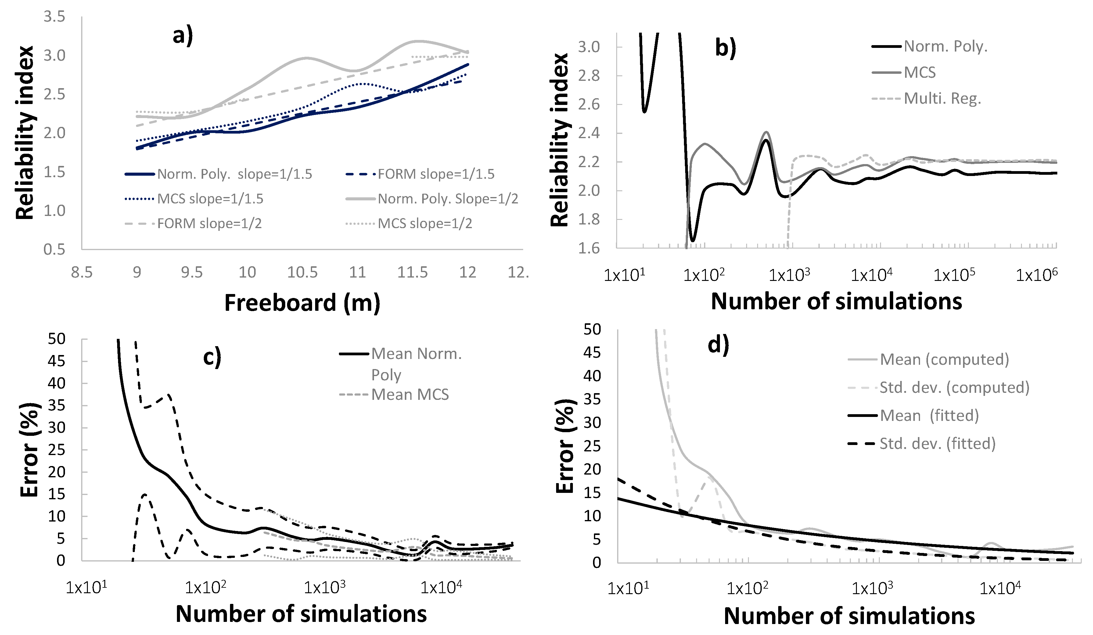
To inspect the variation of β for different F_c values, the FORM is performed by varying the freeboard between 9 m and 12 m and the resulting reliability index is shown in Figure 5a with a black dashed line. As expected, it can be observed that β increases for increasing freeboard; if the slope of the breakwater is increased to tan τ = 1/2 and the FORM is carried out for the same range of F_c, it further increases reliability levels, as shown by the dashed grey line in Figure 5a. These results are used as reference and for comparison purposes, with respect to the results from the normality polynomial and multi-linear regression approaches revisited in this study.

The simulations for this coastal engineering application, used as the basis of the revisited methods, are much more computationally intensive than for the classical and structural examples, because of the dependency between the wave height and period and inclusion of the Longuet-Higgins distribution, which imposes numerical computing for the probability levels (e.g., values from CDFs) and a different method for the sampling. This latter aspect, i.e., the generation of jointly distributed random numbers when a set of x_i variables are dependent, is based on expressing the joint PDF as [22]

$$f_X\left(x\right)=f_{X1}\left(x_1\right)f_{X2}\left(x_2|x_1\right)\dots f_{Xn}\left(x_n|x_1,\dots ,x_{n-1}\right)$$

(33)

with the corresponding CDF given by

$$F_X\left(x\right)=F_{X1}\left(x_1\right)F_{X2}\left(x_2|x_1\right)\dots F_{Xn}\left(x_n|x_1,\dots ,x_{n-1}\right)$$

(34)

Using the previous concepts, and considering a set of values U generated from n independent standard uniformly distributed random variables, the set of dependent random variables can be determined as

$$\{\begin{array}{c}{x}_1=F_{x_1}^{-1}\left(u_1\right)\hfill \\ x_2=F_{x_2}^{-1}\left(u_2|x_1\right)\\ .\\ .\\ .\\ x_n=F_{x_n}^{-1}\left(u_n|x_1,\dots ,x_{n-1}\right)\end{array}$$

(35)

where F⁻¹(•) denotes the inverse of the CDF. The obtaining of this inverse of the CDF can be relatively straightforward for some common probability distributions, where an analytical expression can be used for Equation (35). This is not the case for the Longuet-Higgins distribution. In this case, the jointly distributed random wave height and period must be determined numerically. Figure 6 shows samples of jointly generated random values of wave height and period in the normalized space (for n_sim = 1 × 10³, 5 × 10³; 1 × 10⁴ and 5 × 10⁴). A few contours of the theoretical Longuet-Higgins distribution (i.e., Equation (26)) are also shown in Figure 6; it can be observed that they are in good agreement. The values in the non-normalized space can be obtained simply by recognizing that H_n = H/H_s and T_n = T/T_z.

As mentioned before, the sampling procedure is significantly more time-consuming than for the LSFs in previous sections. Therefore, MCS are sampled only up to 1 × 10⁶ simulations for all the variables of the LSF represented by Equation (25), and the reliability index is determined by employing Equation (17) and Equation (7), only for the case reported in [10] (i.e., F_c = 10 m and tan τ =1/1.5). Nonetheless, results depicted in Figure 5b indicate that the reliability index stabilizes, from approximately n_sim = 1 × 10⁵ and over, to a reliability index practically equal to 2.2 (gray solid line). Therefore, β = 2.2 is adopted as the exact value of the reliability index for the breakwater under overtopping. This value is to be used to assess the error by estimating the reliability index with the normality polynomial approach, and to compare versus the results obtained with the multi-linear regression approach. In fact, the results from these two approaches are also shown in Figure 5b (black solid line for the normality polynomial; grey dashed line for the multi-linear regression approach), where it is observed that the normality polynomial approach converges to a stable value (approximately β = 2.12) from about 2 × 10³ simulations on, leading in average to a slightly smaller reliability index (i.e., in the conservative side) but closer to the exact value than by using the FORM. The multi-linear regression approach (like the MCS and unlike the normality polynomial) requires a minimum number of simulations to be carried out, being this number 1 × 10³ for Figure 5b, but sometimes more simulations are required; nevertheless, when a sufficient large number of simulations is performed (e.g., about 3 × 10⁴ or more in Figure 5b), the results of the multi-linear regression leads to practically the exact β, and the design point and sensitivity factors can also be determined.

For brevity, the coefficients of the polynomials and multi-linear regression, design points and sensitivity factors are not extensively listed in this section, but as an example values are given for a single case of 2 × 10⁴ simulations, which led to coefficients for the normality polynomial of a₀ = −2.164, a₁ = 0.3175, a₂ = −0.0110 and a₃= 0.0028, and for the multi-linear regression of c = 1.4760, b₁ = −0.3382, b₂ = 0.1235, b₃ = −0.5550 and b₄ = −0.0633, as well as sensitivity factors equal to α_Au = 0.5089, α_Bu = −0.1859, α_H = 0.8351, and α_T = 0.0953 and design points equal to x_Au = 1.2874, x_Bu = −0.7263, x_H = 9.3045 m, and x_T = 10.2051 s, which compares very well with the corresponding sensitivity factors computed with the FORM, that are equal to 0.4959, −0.1712, 0.8466, and 0.0900, respectively, and also very well to the design points from FORM equal to 1.2689, −0.7182, 9.0796 m, and 10.1933 s, respectively. These values of sensitivity factors and design points are also very similar with those reported in [10].

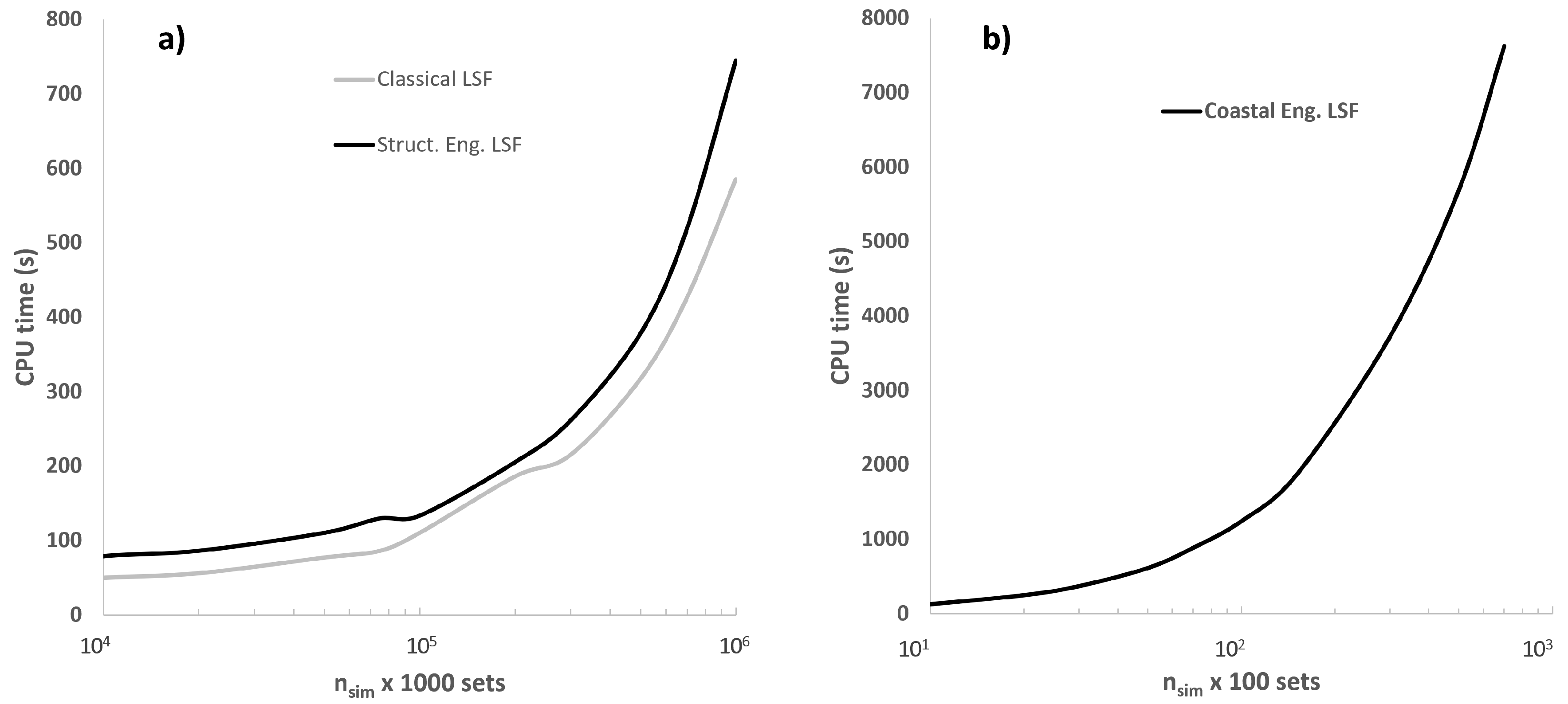
It is noted that Figure 5b corresponds to only one set of simulations for every n_sim, which may vary for different sets of generated random numbers (as shown in Figure 1 and Figure 3), implying an uncertainty in the deviation from the exact value for different number of simulations. This uncertainty is assessed as for the classical and structural LFSs in previous sections, i.e., by computing the errors in the reliability index as per Equation (18) and fitting them to power laws with the mathematical functional form represented in Equations (19) and (20) (or Equations (23) and (24)), but with different values of the parameters. To do so, and unlike the case of the classical LSF and the reinforced concrete beam under flexure moment, not 1000 but only 100 sets of simulations are computed for each n_sim, due to the more extensive required time and computational resources referred to earlier (A comparison in terms of computing time (CPU time), a description and a discussion are given in Appendix B and Figure A2 of the appendix). This leads to the mean errors shown in Figure 5c with a black solid line for the normality polynomial case (including mean values ± one standard deviation indicated in black dashed lines), and with a grey dashed line for the MCS case (including mean values ± one standard deviation indicated in grey dotted lines).

Even though errors reported in Figure 5c exhibit not as a smooth behavior as those observed in Figure 2 and Figure 4 (obtained in an analogous way but for 1000 sets of n_sim), the qualitative trend is fairly similar, especially for mean values and not so small n_sim. Indeed, power laws can be adequately fitted to μ_ε and σ_ε, as shown in Figure 5d by fitting the computed errors from 1 × 10² simulations and over; the mathematical functional form is analogous to that of Equations (23) and (24), except that the constant 1 in Equation (23) is omitted. The obtained fitted parameters are δ = 23.62, γ = 0.2342, κ = 47.94 and τ = 0.4254. As observed in Figure 5d the fitting is very adequate for σ_ε and adequate for μ_ε, albeit only 100 sets of n_sim were employed for the statistics.

From Figure 5c,d similar conclusions to those found before can be drawn, namely, that for decreasing n_sim the MCS tends to deviate more from the exact value than the normality polynomials (in terms of ε), that for decreasing number of simulations the error for the MCS can be unknown and that power laws are adequate to mathematically defined μ_ε and σ_ε for the normality polynomial approach. Therefore, a designer could for instance use the normality polynomial method to compute the reliability index for a reduced number of simulations, whereas accepting an error in the estimation. However, such an error could be estimated if expressions of μ_ε and σ_ε (like the power laws determined in this study) are known.

As an example, in Figure 5a n_sim = 7 × 10² is used for the normality polynomial approach (black solid line) and, as it is shown, this leads to reasonably adequate results (using a fairly small number of simulations) when compared with the FORM and the MCS (also included in Figure 5a with a black dotted line). Moreover, the fitted equations shown in Figure 5d can be used to quantitatively compute the associated error and its standard deviation with respect to the exact reliability index, that is μ_ε = 5.09% and σ_ε = 2.95%. This is strictly applicable only to F_c = 10 m; however, comparable errors may be expected for a range of freeboard values by inspecting Figure 5a. Naturally, the contents of this paper could be extended to investigate how the error changes by varying one or more parameters of the LFSs. In such a case, one would expect that functional forms like those reported in this study can be used to assess ε, but possibly with higher mean errors (and/or standard deviations) for higher reliability levels, because usually more simulations are required for lower probabilities of failure. This could be inferred from Figure 5a, where a last set of calculations is shown by increasing the breakwater slope to 1/2 (dashed and dotted grey lines for the normality polynomial and MCS techniques, respectively), where higher variations of the normality polynomial in relation to the FORM are observed; this higher reliability levels also have the effect of decreasing the ability of the MCS to capture the probability of failure, as also observed in Figure 5a for a wide range of F_c. Additionally, although not shown in Figure 5a, it was observed that the minimum number of simulations required to adequately performed the multi-linear regression increases for higher reliability levels (e.g., larger breakwater slopes).

Overall, results in this section indicate that the revisited simulation-based methods can be also effective for coastal engineering applications.

4. Discussion

Results in the previous section suggest that the two revisited approaches based on simulations, namely, the normality polynomial and the multi-linear regression approaches, are effective in reducing the number of required simulations while adequately computing the reliability index, design point and sensitivity factors. It could be argued that still a relatively large number of simulations are required. However, the computing power is becoming higher every year, and these methods proposed at the end of the 1990s could become a feasible alternative for some complex models two or three decades later.

The power law (Equations (19), (20), (23), and (24)), which describes the precision in computing β for the normality polynomial approach, was found very adequate for the three LSFs considered. Albeit it cannot be concluded that the underlaying error is based on the power law for every possible LSF, since one of LSFs studied here was a simple classical case using only one type of PDF, and the other LSFs were more complex (non-linear functions), with much more random variables and included several PDFs, as well as dependency between variables and the joint Longuet-Higgins distribution, it is reasonable to believe that the error for other LSFs for a wide range of coastal and structural engineering applications could follow the power law. A designer could opt to reduce the number of simulations while accepting an error level (including its uncertainty) by using the power laws as an aid.

The multi-linear regression approach was originally developed to derive the design point and sensitivity factors not obtained when performing MCS; however, it is considered that it can be an alternative by itself to compute β in an accurate way, conditioned on performing enough simulations for a successful regression; the number of simulations can be reduced by increasing the tolerance e. Values reported in this study can be used as a guide.

It is acknowledged that some differences with respect to the present study could be found when other LSFs and applications are used. However, the values reported in this study could be used for guidance, and it is believed that the power law may hold in many coastal and structural engineering applications, since the normality polynomials are based in strong mathematical foundations, as referenced before; nevertheless, future research to further inspect the findings in this study is recommended by using mathematical LSFs considered as benchmark in the literature, but also more ultimate and serviceability LSFs for other coastal and structural engineering applications. It is also believed that the revisited methods and the findings in this study can be exported to other engineering fields if practical applications can be posed as a capacity–demand problem and when extensive simulations are required, including system reliability (for instance for reinforced concrete frame buildings, among many other possibilities). Future research could also include a systematic study for the multi-linear regression approach by varying the tolerance, for given number of simulations, so that the number of MCS can be limited to a minimum while guaranteeing the obtaining of adequate reliability-related values.

If more LSFs are investigated in future studies, perhaps it could be possible to infer general bounds for a wider applicability of the findings in the present study.

5. Conclusions

Two reliability methods based on simulations are revisited. One method fits normality polynomials to the simulated data with fractile constraints, and the other approximates the linearized limit state surface at the design point using multi-linear regression; for the latter, a slight modification is proposed. Three limit state functions, a very simple one, other for a structural engineering application and another for a coastal engineering application, are employed.

The most relevant findings of this study are that for the normality polynomial approach, a power law was found to adequately represent the mean and standard deviation of the error in the estimated reliability index as a function of the number of simulations. It could be used as an aid for decision makers to select a precision level (quantitatively) associated to a selected reliability index, thus reducing the number of required simulations by expressively accepting an error level. Additionally, it is found that the multi-linear regression approach is an excellent option to obtained accurate reliability levels, although a sufficiently large number of simulations is required (not prohibitive though). It also has the advantage that the design point and sensitivity factors are determined.

Other findings in this study are:

• When the normality polynomial approach is used, the reliability index is dependent on the generated random numbers of each run, but it becomes stable for a large number of simulations.
• The reliability index cannot always be determined with the Monte Carlo simulations, while the opposite occurs when normality polynomials are used, although significant deviations from the exact value are observed for small numbers of simulations. In general, for an intermediate number of simulations (e.g., 1 × 10³), the fitted normality polynomials lead to a better estimate of the reliability index than the Monte Carlo simulations.
• When the mean relative error and its standard deviation are computed for the reliability index (compared to the exact value), for decreasing number of simulations the Monte Carlo simulation approach tend to larger mean errors and standard deviations than the normality polynomial approach.
• 3rd-order normality polynomials were mostly used; when 4th order ones are used, the fitting leads to comparable results.
• When the multi-linear regression approach is considered, a minimum number of simulations is required for successfully performing the regression (in the order of 10⁴ to 10⁵simulations), but once this is ensured, a very precise reliability index is obtained (more precise than by using the first order reliability method (FORM)), and the design point and sensitivity factors are also determined and in good agreement with those determined with the FORM.
• If the tolerance for the multi-linear regression approach is increased (i.e., if a wider range in the nearest of the failure surface is stipulated to gather the vectors of simulated data), the number of simulations can be reduced.

References

1. Maliki, M.; Sudret, B. Surrogate-assisted reliability-based design optimization: A survey and a unified modular framework. Struct. Multidiscip. Optim. 2019, 60, 2157. [Google Scholar]
2. Straub, D.; Schneider, N.; Bismut, E.; Kim, H. Reliability analysis of deteriorating structural systems. Struct. Saf. 2020, 82, 101877. [Google Scholar] [CrossRef]
3. Leira, B.; Thöns, S.; Faber, M.H. Reliability assessment of a bridge structure subjected to chloride attack. Struct. Eng. Int. 2018, 28, 318–324. [Google Scholar] [CrossRef]
4. Gong, C.; Zhou, W. Importance sampling-based system reliability analysis of corroding pipelines considering multiple failure modes. Reliab. Eng. Syst. Safe. 2018, 169, 199. [Google Scholar] [CrossRef]
5. Huang, P.; Huang, H.-Z.; Huang, T. A Novel Algorithm for Structural Reliability Analysis Based on Finite Step Length and Armijo Line Search. Appl. Sci. 2019, 9, 2546. [Google Scholar] [CrossRef] [Green Version]
6. Biagi, V.D.; Kiakojouri, F.; Chiaia, B.; Sheidaii, M.R. A Simplified Method for Assessing the Response of RC Frame Structures to Sudden Column Removal. Appl. Sci. 2020, 10, 3081. [Google Scholar] [CrossRef]
7. Marchelli, M.; Biagi, V.D.; Peila, D. Reliability-Based Design of Protection Net Fences: Influence of Rockfall Uncertainties through a Statistical Analysis. Geosciences 2020, 10, 280. [Google Scholar] [CrossRef]
8. Biagi, V.D.; Marchelli, M.; Peila, D. Reliability Analysis and Partial Safety Factors Approach for Rockfall Protection Structures. Eng. Struct. 2020, 213, 110553. [Google Scholar] [CrossRef]
9. Naseri, M.; Barabady, J. An Expert-Based Model for Reliability Analysis of Arctic Oil and Gas Processing Facilities. ASME J. Offshore Mech. Arct. Eng. 2016, 138, 051602. [Google Scholar] [CrossRef]
10. Losada, M.A. ROM 0.0, Puertos del Estado Level II and III Verification Methods. In General Procedure and Requirements in the Design of Harbor and Maritime Structures, Part I, 1st ed.; Puertos del Estado: Madrid, Spain, 2002; Volume 1, pp. 160–185. [Google Scholar]
11. Hong, H.P. Application of polynomial transformation to normality in structural reliability analysis. Can. J. Civ. Eng. 1998, 25, 241. [Google Scholar] [CrossRef]
12. Hong, H.P.; Nessim, M. The development of a design point and sensitivity factors from simulation results. In Proceedings of the Sixth International Conference on Applications of Statistics and Probability in Civil Engineering, CERRA-ICASP 6, Mexico City, Mexico, 17–21 June 1991; pp. 313–319. [Google Scholar]
13. Hong, H.P.; Lind, N. Approximate reliability analysis using normal polynomial and simulation results. Struct. Saf. 1996, 18, 329. [Google Scholar] [CrossRef]
14. Lima-Castillo, I.F.; Gómez-Martínez, R.; Pozos-Estrada, A. Methodology to Develop Fragility Curves of Glass Façades under Wind-Induced Pressure. Int. J. Civ. Eng. 2019, 17, 347. [Google Scholar] [CrossRef]
15. Hall, P. Inverting an Edgeworth expansion. Ann. Stat. 1983, 11, 569. [Google Scholar] [CrossRef]
16. Kendall, M.; Stuart, A.; Ord, J.K. Kendall’s Advance Theory of Statistics; Oxford University Press: New York, NY, USA, 1987; Volume I. [Google Scholar]
17. Madsen, H.O.; Krenk, S.; Lind, N.C. Methods of Structural Safety; Prentice-Hall, Inc.: Englewood Cliffs, NJ, USA, 1986. [Google Scholar]
18. Lind, N.C. Information Theory and maximum product spacings estimation. J. R. Stat. Soc. B 1994, 56, 341–343. [Google Scholar] [CrossRef]
19. Lind, N.C. Statistical method for concrete quality control. In Proceedings of the 2nd International Colloquia on Concrete in Developing Countries, Bombay, India, 3–8 January 1998; Volume 1, pp. 21–26. [Google Scholar]
20. Longuet-Higgins, M.S. On the Joint Distribution of Wave Periods and Amplitudes in a Random Wave Field. Proc. R. Soc. Lond. 1983, 389, 241. [Google Scholar]
21. Rosenblueth, E.; Esteva, L. Reliability basis for some Mexican codes. Am. Concr. Inst. Spec. Publ. 1972, 31, 1–42. [Google Scholar]
22. Hong, H.P. Risk Analysis and Decision Making in Engineering; Course Notes; Western University: London, ON, Canada, 2008; 194p. [Google Scholar]
23. García-Soto, A.D.; Hernández-Martínez, A.; Valdés-Vazquez, J.G. Reliability analysis of reinforced concrete beams subjected to bending using different methods and design codes. Struct. Eng. Int. 2017, 27, 300–307. [Google Scholar] [CrossRef]
24. American Concrete Institute (ACI). Building Code Requirements for Structural Concrete; ACI 318-14; American Concrete Institute (ACI): Farmington Hills, MI, USA, 2014. [Google Scholar]
25. Zhang, H.D.; Soares, C.G. Modified Joint Distribution of Wave Heights and Periods. China Ocean Eng. 2016, 30, 359. [Google Scholar] [CrossRef]
26. Nowak, A.S.; Collins, K.R. Reliability of Structures, 1st ed.; Mc Graw-Hill: Boston, MA, USA, 2000; pp. 120–129. [Google Scholar]
Figure 1. Reliability index as a function of the number of simulations. (a), (b), (c) and (d) are different runs for the MCS.
Applsci 10 08176 g001
Figure 2. Deviations from the exact reliability index as percentage error.
Applsci 10 08176 g002
Figure 3. Reliability index as a function of the number of simulations for RCB. (a), (b), (c) and (d) are different runs for the MCS.
Applsci 10 08176 g003
Figure 4. Deviations from the exact reliability index as percentage error for RCB; (a) rV/D = 0.4 and (b) rV/D = 2.0.
Applsci 10 08176 g004
Figure 5. Reliability of breakwater and error estimation in the reliability index. (a) Reliability index as a function of Fc; (b) Reliability index as a function of nsim; (c) Computed error for the reliability index; (d) Fitted mean and standard deviation for the error in the reliability index estimation.
Applsci 10 08176 g005
Figure 6. Randomly generated joint values of Hn and Tn for (a) 1 × 10³, (b) 5 × 10³, (c) 1 × 10⁴, and (d) 5 × 10⁴ simulations.
Applsci 10 08176 g006