Abstract
Stock performance prediction is one of the most challenging issues in time series data analysis. Machine learning models have been widely used to predict financial time series during the past decades. Even though automatic trading systems that use Artificial Intelligence (AI) have become a commonplace topic, there are few examples that successfully leverage the proven method invented by human stock traders to build automatic trading systems. This study proposes to build an automatic trading system by integrating AI and the proven method invented by human stock traders. In this study, firstly, the knowledge and experience of the successful stock traders are extracted from their related publications. After that, a Long Short-Term Memory-based deep neural network is developed to use the human stock traders’ knowledge in the automatic trading system. In this study, four different strategies are developed for the stock performance prediction and feature selection is performed to achieve the best performance in the classification of good performance stocks. Finally, the proposed deep neural network is trained and evaluated based on the historic data of the Japanese stock market. Experimental results indicate that the proposed ranking-based stock classification considering historical volatility strategy has the best performance in the developed four strategies. This method can achieve about a 20% earning rate per year over the basis of all stocks and has a lower risk than the basis. Comparison experiments also show that the proposed method outperforms conventional methods.
1. Introduction
Stock performance prediction is one of the most challenging issues in time series data analysis. How to accurately predict stock performance changing is an open question with respect to the financial world and academia field. Stock performance prediction is a difficult task, due to the complexity and dynamic of the markets and many inexplicit, intertwined factors involved. Economic analysts and stock traders are the earliest pioneers who perform the prediction of stock performance. In the past several decades, thousands of books in stock trading have been published.
Many economic analysts and stock traders have studied the historical patterns of financial time series data and have proposed various methods to predict stock performance. In order to achieve a promising performance, most of these methods require careful selection of index variables and finding the sharing features among the distinguished stocks. William J. O’Neil and M. Weinstein are two representatives of successful traders. They summarized their stock trading experience in the publications [1,2,3,4]. William J. O’Neil’s CAN SLIM method has a huge following, and also performed well in American Association of Individual Investors (AAII)’s implementation of his model [5]. M. Minervini revealed the proven, time-tested trading system he used to achieve triple-digit returns for five consecutive years, averaging 220% per year [6]. Many followers referred to their methodology in stock trading due to their remarkable achievement.
On the other hand, machine learning models, such as Artificial Neural Networks (ANNs) [7,8,9,10,11,12], Support Vector Regression (SVR) [13,14,15], Genetic Algorithms (GA) [16], as well as hybrid models [17] have been widely used to predict financial time series during recent decades. In addition, the time-series problem considers Dynamic Time Warping (DTW) that handles scaling and shifting, which is common in the stock market. The recently developed DTW Network is an algorithm candidate for financial time series data processing [18]. Ramos-Requena et al. [19] used the Hurst exponent to measure the correlation and co-movement between two different series. Krollner et al. [20] surveyed papers using machine learning techniques for financial time series forecasting based on technique categories, such as ANN-based, evolutionary and optimization techniques, and multiple/hybrid methods. Cavalcante et al. [21] provided a comprehensive overview of the most important primary studies, which cover techniques such as ANN, SVM, hybrid mechanisms, optimization, and ensemble methods. The surveys indicate that the approaches differ regarding the number and types of variables used in modeling financial behavior; however, there is no consensus on which input variables are the best to be used. In addition, it is important to note that there is no well-established methodology to guide the construction of a successful intelligent trading system. The profit evaluation of the proposed methods when used in real-world applications are generally neglected [21].
Recently, deep learning, as an advanced version of ANN, has attracted attention in the machine learning field because of its high performance in areas such as image recognition and speech recognition. In the field of financial forecasting, a similar new trend considers that a deep neural network has the possibility to increase the accuracy of stock market prediction [22,23]. There are two main deep learning approaches that have been used in stock market prediction: Recurrent Neural Networks (RNN) and Convolutional Neural Networks (CNN). Rout et al. made use of a low complexity RNN for stock market prediction [24]. Pinheiro et al. explored RNN with character-level language model pre-training for both intraday and interday stock market forecasting. The proposed automated trading system that, given the release of news information about a company, predicted changes in stock prices [25]. Li et al. adopted the Long Short-Term Memory (LSTM) neural network, which is an improved version of RNN, and incorporates investor sentiment and market factors to analyze the irrational component of stock price [26]. Nelson et al. studied the usage of LSTM networks to predict future trends of stock prices based on the price history, alongside with technical analysis indicators [27]. Bao et al. presented a deep learning framework where wavelet transforms (WT), stacked autoencoders (SAEs), and LSTM are combined for stock price forecasting [28]. Fischer et al. used deep learning, random forests, gradient-boosted trees, and different ensembles as forecasting methods on all S&P 500 constituents from 1992 to 2015. One key finding in their research is that LSTM networks outperform memory-free classification methods [29]. In order to show accountability to their customers, Nakagawa et al. proposed to approximate and linearize the learned LSTM models by layer-wise relevance propagation [30].
Compared to RNN and LSTM, there are a relatively few examples of applying CNN for stock market prediction. Sezer et al. proposed a novel algorithmic trading model CNN-TA using a 2-D convolutional neural network based on 2-D images converted from financial time series data [31]. Zhou et al. proposed a generic framework employing LSTM and CNN for adversarial training to forecast high-frequency stock market [32]. On the whole, the LSTM network is the most widely used deep learning technology for stock performance prediction.
As mentioned above, automatic trading systems that use Artificial Intelligence (AI) have become a commonplace topic, but there are few examples that successfully leverage the proven method invented by human stock traders to build automatic trading systems. The first contribution of this study is the development of an intelligent trading system by integrating AI and the knowledge of human stock traders. In this study, the important index variables suggested by economic analysts and stock traders are used in a deep neural network to predict future stock performance. The second contribution of this study is the verification of the effectiveness of the knowledge of human stock traders and various investment strategies for constructing a successful intelligent trading system. In this study, what index variables are the most significant, and how to perform the stock performance prediction to maximize earning and minimize the risk of investment are investigated. This study is focused on Japanese stock data to explore a reliable investment algorithm for the Japanese stock market. This also aims to verify whether the method invented based on United State (US) stocks is also effective in Japanese stocks, because the traders William J. O’Neil and M. Minervini summarize their experience based on US stocks.
The rest of the paper is organized as follows: Section 2 describes the important index variables and four strategies for stock classification. Section 3 presents the proposed deep neural network to classify the distinguished stocks with good performance. Section 4 shows the evaluation of the proposed systems. Finally, Section 5 concludes this paper.
2. Important Index Variables and Stock Classification
2.1. Important Index Variables for Stock Performance Prediction
In the current stock market, there are hundreds of index variables indicating the value of a stock from different aspects. Professional analysts and stock traders have tried hard to find the correlation between variables and the future performance of stocks. William J. O’Neil and M. Minervini provided many important points and rules for successful stock trading [1,2]. Table 1 lists the 21 index variables (are also called features) that are the most frequently used for recognizing the distinguished stocks in their related publications [1,2].

Table 1.
Important index variables for stock performance prediction.
Among the most important issues in the development of an intelligent trading system is to decide what features should be used for stock performance prediction. One way is just following the suggestions of human stock traders and feeding all features into the developed system. In addition to using all these suggested features, this study presents a feature selection test and verifies the effectiveness of those features. Based on the definition and characteristic of the features, the 21 features are categorized into four groups: price-related features, trading volume features, company financial status-related features, and others. The results of the feature selection test are discussed in Section 4.
In this study, the related data of the important indices with a weekly resolution are downloaded from the stock database and these important features are used as the input of the deep learning algorithm. Daily price-related data and daily trading volume data are also used as the input data of the deep learning algorithm because these two kinds of data (price and trading volume) are the most important for the prediction of stock price from the viewpoint of human stock traders. Using the additional daily resolution data can avoid missing significant dynamic in each week. When the weekly and daily data are used together, the two kinds of data should be synchronized based on time. The solution for data synchronization is explained in Section 3.
2.2. Definition of Positive Samples for Stock Classification
One of the simplest ways of constructing an intelligent trading system is to employ the binary classification algorithm to classify all stocks as two groups: positive samples which are the stocks with good future performance, and negative samples which are the rest of the stocks. This study presents four strategies for classification, and evaluates the strategies from the aspects of both earning rate and risk of investment.
2.2.1. Constant Threshold-Based Stock Classification
Fund managers are concerned about the rising rate of stock price—expressed in Equation (1). For example, if the price rising rate of a stock could surpass a threshold in the next 12 weeks, this stock could be a good candidate for investment. In Equation (1), is the closing price in the current week, and denotes the highest price in the next 12 weeks. In this constant threshold-based stock classification, is used to classify stocks. It means that if of a stock is higher than the threshold, the stock will be defined as a positive sample in the stock classification; otherwise, the stock is a negative sample. In this study, 70% was chosen as the threshold based on the experience of fund managers. If the developed intelligent trading system uses the constant threshold-based method to select stocks, the system will simply predict whether of the stock is over the threshold or not. The system will buy the positive stock in the current week, and sell the positive stock when its reaches the threshold in the next 12 weeks.
2.2.2. Ranking-Based Stock Classification
Because the situation of the market is different every year, in a “good” year, many stocks have good performance and have a high price rising rate. In a “bad” year, the number of stocks with a high price rising rate becomes fewer. In this case, the investment will focus on fewer stocks if the constant threshold method is used for selecting stocks. However, it is necessary to maintain the number of selected stocks and distribute the investment in different stocks to reduce risk.
This study proposes the second strategy in the stock classification. All the stock samples are ranked based on the rising rate expressed in Equation (2), then the top x% samples are defined as positive samples and the rest (100 − x)% of the samples are negative samples. In Equation (2), is the closing price in the current week, and denotes the closing price after 12 weeks. In this ranking-based stock classification, is used to classify the stocks. The value of x was empirically decided as 10 in this research. When the developed intelligent trading system uses this method to select stocks, the system will predict whether the stock is ranked as the top 10% or not, and select the 10% stocks as the positive samples for investment. In this method, there is no constant threshold to decide whether the stocks are in the top 10% or not; therefore, it is impossible to use the strategy of the constant threshold-based method (sell the positive stock when of the stock reaches the threshold) for trading. In this method, the developed intelligent trading system will predict whether the of the stock is in the top 10%, and keep the detected top 10% stocks for 12 weeks before selling them. Therefore, is defined as the price rising rate after 12 weeks, which is different from Equation (1).
2.2.3. Constant Threshold-Based Stock Classification Considering Historical Volatility
In addition to the price rising rate, volatility is also a factor that needs to be considered in the investment. It is necessary to select the stocks which have both a high price rising rate and low volatility. Therefore, this study proposes the third strategy: constant threshold-based stock classification considering historical volatility. In this method, the target rate is defined as Equation (3).
where can be calculated using Equation (1), and is a vector which includes the daily closing price in the past 12 weeks. is the standard deviation of the normalized price in the past 12 weeks. The value of can indicate the historical volatility. In this method, if of a stock is higher than a threshold, the stock will be defined as a positive sample in the stock classification; otherwise, the stock is a negative sample. In this study, 8 was chosen as the threshold based on the experience of fund managers. When the developed intelligent trading system uses this strategy, the system will predict whether of the stock is over the threshold or not. The system will buy the positive stock in the current week, and sell the positive stock when of the stock reaches the threshold in the next 12 weeks.
2.2.4. Ranking Threshold-Based Stock Classification Considering Historical Volatility
Similar to the idea in the second strategy, it is also possible to develop the ranking threshold-based stock classification considering historical volatility. In this method, the target rate is defined as Equation (4).
where can be calculated using Equation (2). The developed intelligent trading system will predict whether of the stock is in the top 10%, and keep the detected top 10% stocks for 12 weeks before selling them.
The designed four strategies are summarized in Table 2. Section 4 presents the performance of the stock trading system developed based on the proposed 4 strategies.
Table 2.
Summary of the proposed four strategies for stock classification.
3. Deep Neural Network-Based Model for Stock Performance Prediction
3.1. Long Short-Term Memory Networks
Long Short-Term Memory networks—usually just called “LSTMs”—are a special kind of RNN equipped with a special gating mechanism that controls access to memory cells. Since the introduction of the gates, LSTM and its variant have shown great promise in tackling various sequence modeling tasks in machine learning—e.g., natural language processing, image captioning, and speech recognition. Basically, a LSTM unit consists of an input gate, a forget gate, and an output gate. The architecture of an LSTM unit is shown in Figure 1.
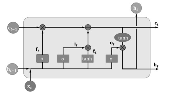
Figure 1.
Visualization of a Long Short-Term Memory (LSTM) unit.
Suppose that is the input and is the hidden output from the last time step t-1, the input gate decides how much of the new information will be added to the cell state , and generates a candidate by:
where can be thought of as a knob that the LSTM learns to selectively consider for the current time step. is the logistic sigmoid function and is tanh. Generally, W terms denote weight matrices (e.g., is the matrix of weights from the input to the input gate), and b terms are the bias vectors. The forget gate decides how previous information will be kept in the new time step, and is defined as:
Then, the cell state is updated by:
where is the element-wise product of the vectors. Then, the output gate uses the output to control what is then read from the new cell state onto the hidden vector as follows:
In this study, the functional LSTM(·,·,·) is used as shorthand for the LSTM model in Equation (11):
where W and b include the weight matrices and bias vectors indicated in Equations (5)–(9). The value of W and b are determined in the training step.
3.2. Concatenated Double-Layered LSTM for Stock Performance Prediction
This study proposes a LSTM-based network to predict the future performance of stocks by classification. The proposed network classifies stocks into two categories (buying or not) based on the historical sequence data. The “Many to one” model has been widely used in sequence data processing. To fully use the memory and forget ability of LSTM, our proposed network is also a “many to one” model. The architecture of the proposed classification network is shown in Figure 2. This means that when classifying the stocks into two categories (buying or not), the historical sequence data from time t− n to t: are input into the network together. In the proposed network, n was empirically decided as 52 by considering the experience of professional traders.
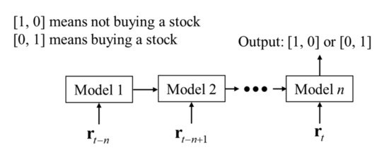
Figure 2.
“Many to one” architecture for the classification of stocks.
Figure 3 corresponds to the model in Figure 2. It shows the architecture of the model block. There are double-layered LSTMs. Finally, the output is connected with the last LSTM layer. Here, denotes the input data at week t. The double-layered LSTM model can be explained by:
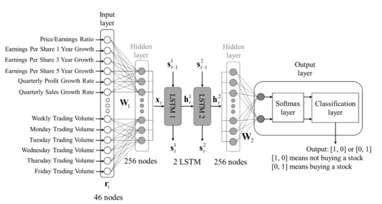
Figure 3.
Architecture of double-layer LSTM model for the stock performance prediction.
In Figure 3, stands for . To reduce the complexity of the task, in this study, a binary-class classification system was developed for stock performance prediction. This means that the classification system is expected to recognize two categories. Therefore, the output of the final hidden layer connects two nodes to indicate the probabilities for two categories, the probabilities can be estimated from the output of the second LSTM layer as:
where is a weight matrix from the hidden layer to the output layer, and is the bias vector. is a vector to indicate the probability of the sample for two categories: 0 and 1. The category “0” means not buying a stock, and the category “1” means buying a stock. The softmax layer and classification layer are responsible for normalization and category selection which are explained in the following equations:
The double-layer LSTM model can predict whether the automatic trading system should buy or not buy a stock, given the past 52-week history information of that stock. The output of the double-layer LSTM model could be [1, 0] or [0, 1]. [1, 0] means not buying the stock, and [0, 1] means buying the stock. The output ([1, 0] or [0, 1]) is decided in the category selection block based on the comparison of the normalized probabilities provided by the softmax layer. If the probability of category “0” (not buying a stock) is higher than the probability of category “1” (buying a stock), the output is [1, 0]. Otherwise, the output will be [0, 1].
In the training of the network, is used as the sample data because of the “many to one” architecture. The training algorithm automatically adjusts the parameters in the model based on the principle of the gradient descent. In the training, the loss function is a cross entropy:
where, N is the number of samples in the training dataset. is the row vector format ground truth for sample j. The objective of the training process is to minimize the value of Loss Function Equation (17). In Figure 3, both weekly and daily data are used as the input of the LSTM-based deep learning network; one weekly datum can be connected with five daily data from Monday to Friday.
Considering the particularity of the stock classification, the mistakes in the classification have different practical meanings. For example, in comparison to false negative (stocks with good performance are missed in detection), the false positive (stocks are incorrectly detected as good performance stocks) has a higher risk in the real investment. It is possible to give a higher weighting to false positive in the loss function to force the training to reduce the false positive. For example, the ratio of the weighting of false negative and false positive could be 1:2, 1:3, and so on. Therefore, the loss function is reformed as Equation (18). In the experiments, this research presents an attempt to find the best option for parameter in order to achieve good performance of the developed trading system.
4. Experiment Results
4.1. Experiment Setup and Evaluation Criteria
In this study, a deep neural network was adopted and 52-week historical data of features were used as the input of the deep neural network for a binary classification. For example, when the system performed the classification on 2018/04/01 to select the stocks with good performance in the next 12 weeks, the historical data of 2017/04/03–2018/04/01 (52 weeks) were input into the deep neural network. The ground truth of each historical data is binary data: buying the stock or not, when talking about the future 12-week performance. Because the data are organized weekly, one stock can provide 52 samples per year. For example, the historical data of the samples could be 2017/04/03–2018/04/01, 2017/04/10–2018/04/08, 2017/04/17–2018/04/15, …, 2018/03/27–2019/03/25. The future 12-week data of these samples are 2018/04/01–2018/06/25, 2018/04/08–2018/07/02, 2018/04/15–2018/07/09, …, 2019/03/25–2019/06/17, as shown in Figure 4. In the following description, this paper uses the time of the end of data to denote the 52-week length historical data input into the deep neural network. For example, “2018/04/01” denotes the historical data “2017/04/03–2018/04/01”.
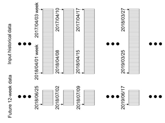
Figure 4.
The 52 samples extracted from one stock data.
In this study, the training dataset, validation dataset, and test dataset were separated based on the year and month as shown in Table 3. In order to verify the repeatability of the proposed method, this study presents the evaluation of the different datasets. For example, when the system was tested on the dataset of the period from 2018/04/01 to 2018/09/30 (as indicated in the final row of Table 3), the data from 2017/04/01 to 2017/12/31 were used for validation, and the data from 2001/04/01 to 2016/09/30 were used for training. The datasets in each row of Table 3 are considered as one set. Averagely, the number of samples in each training, validation, and test dataset is about 450,000, 45,000, and 30,000, respectively. It is important to note that there is no overlap among training, validation, and test data in each set. The basic process in the evaluation of each set of datasets is to use the training dataset for training the model and obtaining multiple classifiers. After that, the best classifier is selected based on the validation dataset. Finally, the selected classifier is evaluated in the test dataset. This process was conducted on each set of datasets to demonstrate the repeatability of the proposed methods.
Table 3.
Training dataset, validation dataset, and test dataset for repeatability evaluation.
The training dataset was used to train the model. Training is an iteration process with multiple epochs. One epoch means that all training data have been used once for backpropagation. In this study, the number of epochs was set as 50, because 50 epochs are enough for the convergency of the training process. The training process output one classifier after each epoch. Therefore, 50 different classifiers were generated after 50 epochs. Theoretically, the final classifier should have the best performance. However, the performance of the classifiers did not change too much in the training process. One reason is that enough training data were provided for the deep learning algorithm. After several epochs, the training processing converged, and the parameters of the classifier were optimal.
However, how to choose the best classifier is a problem. In this study, a validation dataset was used to choose the best classifier. As shown in Table 3, the validation dataset is the most recent year before the test dataset. In addition, there is three-month gap between the validation data and test data. When the system works on the day of 2018/03/31 and predicts the future of stocks in the next 12 weeks, the validation dataset should be the data from 2017/04/01 to 2018/03/31. However, the future 12-week data for the historical data from 2018/01/01 to 2018/03/31 are not available on the day 2018/03/31. Therefore, the data from 2018/01/01 to 2018/03/31 cannot be used for validation, and the validation dataset has a 9-month period.
In addition, as described in Section 3, the low false positive value is also expected in the stock selection. Therefore, when choosing the classifier, it is also necessary to consider which one has a low false positive value and maintain the high true positive value at the same time. In this study, the following best precision criterion was adopted to select the classifier in the validation dataset:
where TP is the number of true positive samples and FP is the number of false positive samples.
In the repeatability evaluation, the test dataset had half a year period, and the validation dataset had a 9-month period. The training dataset is the data excluding the test and validation dataset. For example, when the test dataset is data from 2011/04/01 to 2011/09/30, the validation dataset is data from 2010/04/01 to 2010/12/31. In this case, the training dataset was the data from 2001/04/01 to 2010/03/31 and the data from 2012/10/01 to 2018/09/30. In this study, future data after the test data were used for training, because the deep learning needs huge training data to achieve good performance. Using the data after the test data period increases the number of training samples. It is important to note that there is a one-year gap from the end of the test data period to the training data period, because excluding the data in that one year can strictly guarantee that any part of the test data is not used in the training.
In this study, True Positive Rate (TPR, Recall), True Negative Rate (TNR), Average Correction Rate (ACR), and Precision were used to evaluate the performance of the developed prediction systems. The evaluation criteria are denoted in Equations (20)–(23):
where P is the number of all positive samples, and N is the number of all negative samples. TP is the number of true positive samples, FP is the number of false positive samples, TN is the number of true negative samples, and FN is the number of false negative samples.
In addition to the four criteria, the average maximum price rising rate of stocks and average maximum price decreasing rate of stocks were also used in the evaluation. Moreover, this study also presents a simulation of stock trading to evaluate the performance of the proposed methods, and the details of the simulation are presented in each following each subsection.
4.2. Results of Constant Threshold-Based Stock Classification
In the evaluation of the method of constant threshold-based stock classification, two factors should be discussed: parameter in Equation (18), and features in Table 1. Table 4 shows the performance of the classification using all features and (1:1) values.
Table 4.
Constant threshold-based stock classification with threshold 70%, (1:1), all features.
The first column indicates the time period of the test dataset. True negative rate, true positive rate (recall), average correction rate, and precision are listed from the second to fifth columns. The average of the maximum rising rate of detected good performance stocks and all stocks are demonstrated in the sixth and seventh columns. The average of the maximum decreasing rate of detected good performance stocks and all stocks are shown in the eighth and ninth columns.
Moreover, this study also presents a simulation of a real stock trading system. In the case of the binary-class classification system using 70% rising rate threshold, the system sets up a 70% rising rate as the selling point. The system will firstly buy all selected stocks. If a selected stock (detected positive sample) achieves 70% rising rate, the system sells it immediately. Otherwise, the stock is kept and sold by the end of 12 weeks. The tenth and eleventh columns of Table 4 show the earning rate of the simulated stock trading system. In addition, the twelfth column of Table 4 provides the basis of all stocks. The basis is the average earning rate from present to 12 weeks later.
In addition, the other two criteria are used in the evaluation of risk: Sharpe ratio with trading on selling point and Sharpe ratio without trading on selling point. The two criteria are defined as Equations (24) and (25):
where CP is the closing price in the current week, is the price when selling the stock, and is the close price after 12 weeks. In Equation (24), is a vector which includes the daily closing price from the current week to selling. is a vector which includes the daily closing price in the next 12 weeks.
In fact, the Sharpe ratio without trading on selling point means the stocks will be sold at the end of 12 weeks. The thirteenth and fourteenth columns of Table 4 show the Sharpe ratio with trading on selling point, the fifteenth and sixteenth columns of Table 4 illustrate the Sharpe ratio without trading on selling point. In addition, the average of all tests is listed in the last row of Table 4. This study presents the evaluation of different features and values. Because of the limitation of the page length, Table 5 shows the summary of these evaluations. In this study, the results generated using different values were compared, and then the best values were chosen for the feature selection. The following conclusions can be obtained from the data in Table 5:
Table 5.
Constant threshold-based stock classification with different values and different features (all: all features; price: price-related features; trading volume: trading volume feature; financial status: company financial status-related features).
- (1)
- Values of parameter affect the earning rate.
- (2)
- Price features can provide the best performance compared to all features.
- (3)
- The best earning rate happens when the stock classification uses (1:2), price features. A 2.146% (6.037–3.891%) earning rate per 12 weeks above basis is achieved in constant threshold-based stock classification.
- (4)
- The Sharpe ratio of the detected stock is lower than all stocks, which indicates that the constant threshold-based stock classification method has a relatively high risk in stock classification. The reason for this is that the stock volatility is not considered in this method.
4.3. Results of Ranking-Based Stock Classification
Similar to the constant threshold-based stock classification, this study also presents multiple evaluations for the ranking-based stock classification. In the evaluation, the effect of different values of and input features was tested. In the ranking-based stock classification, the top 10% stocks were considered as positive samples. Table 6 shows results generated using the different configurations. There was no fixed threshold for stock trading; therefore, the simulated stock trading system kept the detected or all stocks until the end of the following 12 weeks and then sold them. Thus, there was no Sharpe ratio with trading. The following conclusions can be obtained from the data in Table 6.
Table 6.
Ranking-based stock classification with different values and different features (all: all features; price: price-related features; trading volume: trading volume feature; financial status: company financial status-related features).
- (1)
- Values of parameter affect the earning rate.
- (2)
- Price and trading volume-related features can provide the best performance compared to all features.
- (3)
- The best earning rate happens when the stock classification uses (1:2), price and trading volume-related features. A 6.984% (10.875–3.891%) earning per 12 weeks above basis is achieved in the ranking-based stock classification.
- (4)
- The Sharpe ratio of the detected stock is lower than all stocks, which indicates the ranking-based stock classification method has a relatively high risk for the stock classification. The reason is that the stock volatility is not considered in this method.
- (5)
- From the aspect of the earning rate, the ranking-based stock classification method is more effective than the constant threshold-based stock classification method.
4.4. Results of Constant Threshold-Based Stock Classification Considering Historical Volatility
Similar to the constant threshold-based stock classification, this study also presents multiple evaluations for the constant threshold-based stock classification considering historical volatility. In the evaluation, the effect of different values of the parameter and input features was tested. Table 7 shows results using different configurations. In the ranking-based stock classification, the threshold for target rate was set as eight to classify positive samples. In the simulated trading system, the target rate eight was set as the selling point. If the stock achieves the target rate eight, it will be sold immediately. Otherwise, the system will keep the stock and sell it by the end of 12 weeks. The following conclusion can be obtained from the data in Table 7.
Table 7.
Constant threshold-based stock classification considering historical volatility using different values and different features (all: all features; price: price-related features; trading volume: trading volume feature; financial status: company financial status-related features).
- (1)
- Values of parameter affect the earning rate.
- (2)
- Price and trading volume-related features can provide the best performance compared to all features.
- (3)
- The best earning rate happens when the stock classification uses (1:1), price and trading volume-related features. A 2.504% (6.395–3.891%) earning per 12 weeks above basis is achieved.
- (4)
- The Sharpe ratio of the detected stock is higher than all stocks, which indicates this method can also reduce risk in stock selection. The reason is that stock volatility is considered in this method.
- (5)
- From the aspects of Sharpe ratio, this method has better performance than the stock classification method without considering historical volatility.
4.5. Results of Ranking-Based Stock Classification Considering Historical Volatility
Similar to the previous methods, this study also presents multiple evaluations for the ranking-based stock classification considering historical volatility. In the evaluation, the effect of different values of parameter and input features was tested. Table 8 shows the results using different configurations. In this method, the top 10% of stocks were considered as positive samples. Table 8 shows a summary of the evaluations. There was no fixed threshold for stock trading; therefore, the simulated stock trading system kept the detected or all stocks until the end of next 12 weeks, then sold them. Thus, there was no Sharpe ratio with trading. The following conclusion can be obtained from the data in Table 8.
Table 8.
Ranking-based stock classification considering historical volatility using different values and different features (all: all features; price: price-related features; trading volume: trading volume feature; financial status: company financial status-related features).
- (1)
- Values of parameter affect the earning rate.
- (2)
- Price and trading volume-related features can provide the best performance compared to all features.
- (3)
- The best earning rate happens when the stock classification uses (1:1), price and trading volume-related features. The method of the ranking-based stock classification considering historical volatility has a 9.044% earning rate per 12 weeks in Japanese stock data from 2011 to 2018. A 5.153% (9.044–3.891%) earning per 12 weeks above basis is achieved in ranking-based stock classification considering historical volatility.
- (4)
- The Sharpe ratio of the detected stock is higher than all stocks, which indicates this method can reduce the risk in stock classification. The value of Sharpe ratio of this method is very similar to its value in the method of the constant threshold-based stock classification considering historical volatility.
- (5)
- By considering both earning rate and Sharpe ratio, the ranking-based stock classification method considering historical volatility is the most effective strategy among the proposed four strategies.
In addition, in this study, the proposed deep neural network-based stock performance prediction method was compared with two conventional methods: Logistic Regression-based classification and Support Vector Machine (SVM)-based classification. This comparison was performed for the ranking-based stock classification considering historical volatility. The comparison in Table 9 shows the proposed method has a higher earning rate and a lower risk than the conventional methods.
Table 9.
Comparison for ranking-based stock classification considering historical volatility.
5. Conclusions
This study presents four strategies for stock classification and performs feature selection to achieve a higher earning rate and lower risk in stock classification. The following points are concluded based on the evaluations and analysis:
- (1)
- Using the ranking method can improve the earning rate above basis.
- (2)
- Using historical volatility information for training can increase the Sharpe ratio and reduce the risk in stock classification.
- (3)
- Using price and trading volume-related features has a better performance than using full features in stock classification.
- (4)
- By considering both earning rate and risk, the ranking-based stock classification method considering historical volatility is the most effective strategy among the proposed four methods. About 5.2% earning rate per 12 weeks over than the basis of all stocks is achieved in the repeatability test. The selected stocks have lower risky than basis.
- (5)
- The proposed deep neural network-based stock performance prediction method has better performance than the conventional methods.
The proposed method can have about 36% (9.044% per 12 weeks) earning rate per year in the Japanese stock market. However, excellent human stock traders have achieved triple-digit returns per year [6]. There is still a gap between the performance of the developed intelligent trading system and the achievements of human stock traders. This paper proposed the use of the classification network to classify the stocks into two categories: buying or not. In the future, a regression network will be developed to predict the exact value of the future price. In this way, the developed trading system is expected to obtain higher earnings.
Author Contributions
Conceptualization, S.K. and S.N.; methodology, S.K., S.N., T.S., Y.K. and Y.G.; data acquisition, T.S. and Y.G.; software, Y.G.; experiment, Y.G.; writing, Y.G.; project administration, S.K. and S.N.; All authors have read and agreed to the published version of the manuscript.
Funding
This research received no external funding.
Conflicts of Interest
The authors declare no conflict of interest.
References
- Minervini, M. Trade like a Stock Market Wizard: How to Achieve Super Performance in Stocks in Any Market. McGraw-Hill: New York, NY, USA, 2013. [Google Scholar]
- Schwager, J.D. Market Wizards: Interviews with Top Traders; Wiley: Hoboken, NJ, USA, 2012. [Google Scholar]
- Schwager, J.D. Stock Market Wizards: Interviews with America’s Top Stock Traders; Harper-Business: New York, NY, USA, 2003. [Google Scholar]
- William, J.O. How to Make Money in Stocks: A Winning System in Good Times and Bad, 4th ed.; McGraw-Hill: New York, NY, USA, 2009. [Google Scholar]
- Book Review of the Successful Investor by William J. O’Neil. Available online: https://whatheheckaboom.wordpress.com/2012/04/23/book-review-of-the-successful-investor-by-william-j-oneil/ (accessed on 1 September 2020).
- Book description of Trade like a Stock Market Wizard: How to Achieve Super Performance in Stocks in Any Market. Available online: https://www.mhebooklibrary.com/doi/book/10.1036/9780071807234 (accessed on 1 September 2020).
- Martinez, L.C.; Da Hora, D.N.; Palotti, J.R.D.M.; Meira, W.; Pappa, G.L. From an Artificial Neural Network to a Stock Market Day-trading System: A Case Study on the BM&F BOVESPA. In Proceedings of the 2009 International Joint Conference on Neural Networks, Atlanta, GA, USA, 14–19 June 2009. [Google Scholar]
- Dhar, S.; Mukherjee, T.; Ghoshal, A.K. Performance Evaluation of Neural Network Approach in Financial Prediction: Evidence from Indian Market. In Proceedings of the 2010 International Conference on Communication and Computational Intelligence, Erode, India, 27–29 December 2010. [Google Scholar]
- Oliveira, A.L.; Meira, S.R. Detecting Novelties in Time Series Through Neural Networks Forecasting with Robust Confidence Intervals. Neurocomputing 2006, 70, 79–92. [Google Scholar] [CrossRef]
- Chen, A.S.; Leung, M.T.; Daouk, H. Application of Neural Networks to an Emerging Financial Market: Forecasting and Trading the Taiwan Stock Index. Comput. Oper. Res. 2003, 30, 901–923. [Google Scholar] [CrossRef]
- Guresen, E.; Kayakutlu, G.; Daim, T.U. Using Artificial Neural Network Models in Stock Market Index Prediction. Expert Syst. Appl. 2011, 38, 10389–10397. [Google Scholar] [CrossRef]
- Sezer, O.B.; Ozbayoglu, A.M.; Dogdu, E. An Artificial Neural Network-based Stock Trading System using Technical Analysis and Big Data Framework. In Proceedings of the SouthEast Conference, Kennesaw, GA, USA, 13–15 April 2017. [Google Scholar]
- Prasaddas, S.; Padhy, S. Support Vector Machines for Prediction of Futures Prices in Indian Stock Market. Int. J. Comput. Appl. 2012, 41, 22–26. [Google Scholar] [CrossRef]
- Bao, Y.; Yang, Y.; Xiong, T.; Zhang, J. A Comparative Study of Multi-step-ahead Prediction for Crude Oil Price with Support Vector Regression. In Proceedings of the IEEE Fourth International Joint Conference on Computational Sciences and Optimization, Yunnan, China, 15–19 April 2011. [Google Scholar]
- Kara, Y.; Acar Boyacioglu, M.; Baykan, O.K. Predicting Direction of Stock Price Index Movement Using Artificial Neural Networks and Support Vector Machines: The Sample of the Istanbul Stock Exchange. Expert Syst. Appl. 2011, 38, 5311–5319. [Google Scholar] [CrossRef]
- Aguilar-Rivera, R.; Valenzuela-Rendón, M.; Rodriguez-Ortiz, J. Genetic Algorithms and Darwinian Approaches in Financial Applications: A Survey. Expert Syst. Appl. 2015, 42, 7684–7697. [Google Scholar] [CrossRef]
- Nayak, R.K.; Mishra, D.; Rath, A.K. A Naive SVM-KNN based Stock Market Trend Reversal Analysis for Indian Benchmark Indices. Appl. Soft Comput. 2015, 35, 670–680. [Google Scholar] [CrossRef]
- Cai, X.; Xu, T.; Yi, J.; Huang, J.; Rajasekaran, S. DTWNet: A Dynamic Time Warping Network. Adv. Neural Inf. Process. Syst. 2019, 32, 11640–11650. [Google Scholar]
- Ramos-Requena, J.P.; Trinidad-Segovia, J.E.; Sánchez-Granero, M.Á. An Alternative Approach to Measure Co-Movement between Two Time Series. Mathematics 2020, 8, 261. [Google Scholar] [CrossRef]
- Krollner, B.; Vanstone, B.; Finnie, G. Financial Time Series Forecasting with Machine Learning Techniques: A Survey. In Proceedings of the 18th European Symposium on Artificial Neural Networks, Bruges, Belgium, 28–30 April 2010. [Google Scholar]
- Cavalcante, R.C.; Brasileiro, R.C.; Souza, V.L.; Nobrega, J.P.; Oliveira, A.L. Computational Intelligence and Financial Markets: A Survey and Future Directions. Expert Syst. Appl. 2016, 55, 194–211. [Google Scholar] [CrossRef]
- Nakagawa, K.; Uchida, T.; Aoshima, T. Deep factor model Explaining Deep Learning Decisions for Forecasting Stock Returns with Layer-Wise Relevance Propagation. In Proceedings of the ECML PKDD 2018 Workshops, Dublin, Ireland, 10–14 September 2018. [Google Scholar]
- Abe, M.; Nakayama, H. Deep Learning for Forecasting Stock Returns in the Cross-section. In Proceedings of the 2018 Pacific-Asia Conference on Knowledge Discovery and Data Mining, Melbourne, Australia, 3–6 June 2018. [Google Scholar]
- Rout, A.K.; Dash, P.K.; Dash, R.; Bisoi, R. Forecasting Financial Time Series using a Low Complexity Recurrent Neural Network and Evolutionary Learning Approach. J. King Saud Univ. -Comput. Inf. Sci. 2017, 29, 536–552. [Google Scholar] [CrossRef]
- Dos Santos Pinheiro, L.; Dras, M. Stock Market Prediction with Deep Learning: A Character-based Neural Language Model for Event-based Trading. In Proceedings of the Australasian Language Technology Association Workshop 2017, Brisbane, Australia, 6–8 December 2017. [Google Scholar]
- Li, J.; Bu, H.; Wu, J. Sentiment-aware Stock Market Prediction: A Deep Learning Method. In Proceedings of the IEEE 2017 International Conference on Service Systems and Service Management, Dalian, China, 16–18 June 2017. [Google Scholar]
- Nelson, D.M.; Pereira, A.C.; De Oliveira, R.A. Stock Market’s Price Movement Prediction with LSTM Neural Networks. In Proceedings of the 2017 International Joint Conference on Neural Networks, Anchorage, AK, USA, 14–19 May 2017. [Google Scholar]
- Bao, W.; Yue, J.; Rao, Y. A Deep Learning Framework for Financial Time Series using Stacked Autoencoders and Long-short Term Memory. PLoS ONE 2017, 12, e0180944. [Google Scholar] [CrossRef]
- Fischer, T.; Krauss, C. Deep Learning with Long Short-term Memory Networks for Financial Market Predictions. Eur. J. Oper. Res. 2018, 270, 654–669. [Google Scholar] [CrossRef]
- Nakagawa, K.; Ito, T.; Abe, M.; Izumi, K. Deep Recurrent Factor Model: Interpretable Non-Linear and Time-Varying Multi-Factor Model. In Proceedings of the AAAI 2019 Workshop on Network Interpretability for Deep Learning, Honolulu, HI, USA, 27–28 January 2019; 2019. [Google Scholar]
- Sezer, O.B.; Ozbayoglu, A.M. Algorithmic Financial Trading with Deep Convolutional Neural Networks: Time Series to Image Conversion Approach. Appl. Soft Comput. 2018, 70, 525–538. [Google Scholar] [CrossRef]
- Zhou, X.; Pan, Z.; Hu, G.; Tang, S.; Zhao, C. Stock Market Prediction on High-frequency Data using Generative Adversarial Nets. Math. Probl. Eng. 2018, 2018, 525–538. [Google Scholar] [CrossRef]
Publisher’s Note: MDPI stays neutral with regard to jurisdictional claims in published maps and institutional affiliations. |
© 2020 by the authors. Licensee MDPI, Basel, Switzerland. This article is an open access article distributed under the terms and conditions of the Creative Commons Attribution (CC BY) license (http://creativecommons.org/licenses/by/4.0/).