Natural Frequency Prediction Method for 6R Machining Industrial Robot

Abstract

The industrial robot machining performance is highly dependent on dynamic behavior of the robot, especially the natural frequency. This paper aims at introducing a method to predict the natural frequency of a 6R industrial robot at random configuration, for improving dynamic performance during robot machining. A prediction model of natural frequency which expresses the mathematical relation between natural frequency and configuration is constructed for a 6R robot. Joint angles are used as input variables to represent the configurations in the model. The quantity and range of variables are limited for efficiency and practicability. Then sample configurations are selected by central composite design method due to its capacity of disposing nonlinear effects, and natural frequency data is acquired through experimental modal test. The model, which is in form of regression equation, is fitted and optimized with sample data through partial least square (PLS) method. The proposed model is verified with random configurations and compared with the original model and a model fitted by least square method. Prediction results indicate that the model fitted and optimized by PLS method has the best prediction ability. The universality of the proposed method is validated through implementation onto a similar 6R robot.

1. Introduction

Due to the rapid development of industrial automation, the global amount of industrial robot keeps increasing significantly in recent years [1], and new applications attract more attention [2,3,4,5]. Because of the multiple degree of freedom, large workspace, and relative low cost, industrial robot becomes a potential alternative of traditional machine tool in hard material drilling [6], boring [7], and milling [8,9] processes, which are not maturely and widely applied.

For machine tool, in the whole workspace, the stiffness and dynamic behavior nearly remain steady, so machining stability and chatter suppression, which are concerned with multiple factors, are research emphasis [10,11,12]. However, for industrial robot, current researches focus on the characteristic of robot itself. Common industrial robot is of open-loop articulated serial structure with six revolute joints (6R); therefore, the stiffness and dynamic performance are much inferior to machine tool, which results in vibration issues and poor surface quality in machining process [13]. Static stiffness issues are studied to avoid the robot deformation in machining, and several stiffness indexes are proposed to evaluate the static stiffness of robot in the workspace [14,15,16,17]. On the other hand, dynamic behavior of robot is studied to evaluate the capacity of dealing with time-variant load in machining process, which may help to suppress vibration [18,19]. As 6R robot realizes movement through adjusting joint angles, dynamic behavior keeps varying with configurations during motion process. For that reason, research object is gradually expanded from one configuration to the whole workspace. Bisu et al. [20] selected three configurations from a linear movement path of a 6R robot with interval of 50 cm for dynamic behavior study and vibration analysis. It was found that different natural frequencies led to dynamic performance variation. Mousavi et al. [21] performed a similar four-point-study and analyzed the change of stability region through modal information. Several configurations may present a linear movement, but the usage of robot should not be such limited. Karim et al. [22] executed modal test with 63 measured points for 23 configurations, through which mode shapes were obtained and approximate distribution of first two step natural frequencies in a plane was depicted. Natural frequency is the vital dynamic parameter in robot machining, but massive tests are inefficient although the accuracy is well ensured. A method was proposed by Glogowski et al. [23] to predict natural frequency in the whole workspace efficiently, in which sample configurations were selected by design of experiment (DoE) method and prediction model was fitted by least square (LS) method with the natural frequency data of sample configurations, but the prediction deviation reached up to 8.9%, making the method inadequate for practical application.

The low order natural frequencies of 6R robot are relatively small and the first order is merely about 10 Hz, which is covered in frequency range of most machining processes, so 6R robot tends to forced vibration during machining processes [24]. To obtain basis for vibration suppression, structure optimization and path planning, low order natural frequencies are particularly concerned among dynamic parameters. It is proposed that low order natural frequencies of robot are decided by the configurations, while the high order natural frequencies are mainly related to the machining system, which do not vary with robot configurations [25], this phenomenon is demonstrated in Figure 1.

Thus, a method to predict natural frequency of 6R industrial robot efficiently and precisely is proposed in this paper. As shown in Figure 2, sample configurations are selected to present the practical workspace (variable range) for fast prediction, and a regression equation fitted and optimized by partial least square (PLS) method is used as prediction model for higher accuracy. A 6R robot, ABB IRB4600, is used to illustrate and validate the method. Another ABB IRB6400 is used verify the universality of proposed method.

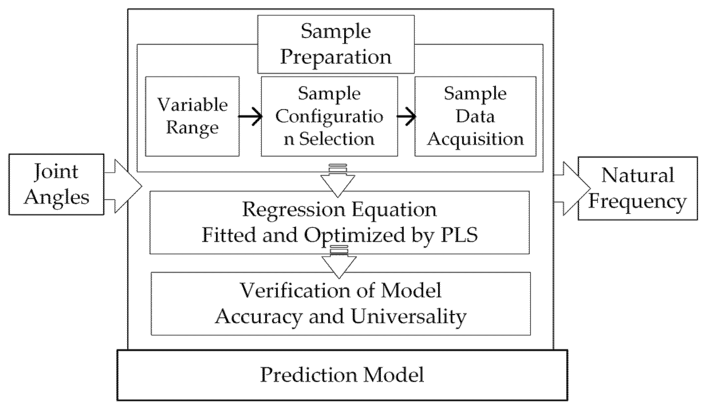
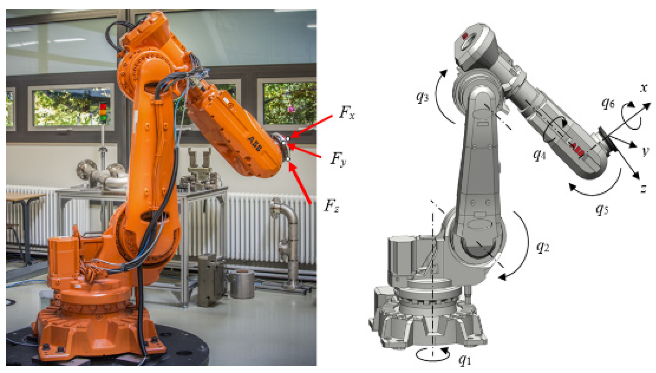
2. Materials and Methods

2.1. Sample Preparation

The axes of 6R robot are noted as a₁, a₂, …, a₆, corresponding joint angles are q₁, q₂, …, q₆. The mapping relation between natural frequency (f_F) and configuration can be expressed as

$$f_{\mathrm{F}}=\mathrm{f}(q_1,q_2,\dots ,q_6),$$

(1)

With samples, a regression equation can be fitted to represent the mapping relation. However, it is unnecessary and inefficient to include the entire workspace of the robot as the configurations near the boundary could not be adopted in machining process. Therefore, range of variables is limited before selecting samples through DoE method. Then natural frequency information of each sample configuration is acquired through modal test.

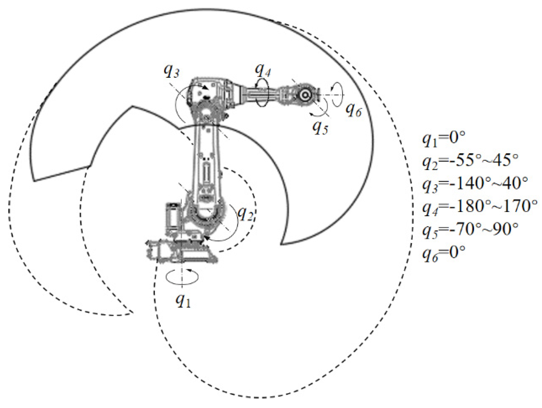
2.1.1. Variable Range Determination

a₁, which is the basic rotation axis of the robot structure, and a₆, which is a 360° rotation axis controlling the flange, are proved to be nonsignificant in changing natural frequency by preliminary researches on 6R robots including KUKA KR60, ABB IRB6400, and IRB 4600. As low order natural frequencies is mainly decided by robot configuration, none end-effector is fixed on the flange in above cases for general research. Hereby, q1 and q6 are excluded from model (q₁ = q₆ = 0° in practice) for the simplification, and q₂–q₅ are applied as variables. Prediction model can be adapted to

$$f_{\mathrm{F}}=\mathrm{f}(q_2,q_3,q_4,q_5),$$

(2)

To ensure the efficiency of model, partial workspace that may cause movement interference in machining process is rejected by simulation software. The variable range is finally determined and shown in Figure 3, where the solid area indicates the new efficient workspace, and the dashed area represents the original workspace.

2.1.2. Sample Configuration Selection

DoE method has advantages in study influence of different factors, especially for basic research of robot machining, e.g., Simoes et al. [26] used DoE to study influence of robot milling parameters. Different types of selection methods are compared in pilot study including three-level full factorial design (3kD), orthogonal experimental design, Box-Behnken design, and central composite design (CCD). The prediction performances of 3kD and CCD are nearly matched and superior to the other two, while CCD demands a much smaller sample amount [23]. Meanwhile CCD owns conspicuous ability in disposing the nonlinear influence that joint angles may lead to natural frequency. Therefore, CCD method is adopted to select sample configurations in this paper, corresponding factors and levels are shown in

Table 1. Factors and Levels of central composite design (CCD).

Factors Levels	q2 (Deg)	q3 (Deg)	q4 (Deg)	q5 (Deg)
−1	−55	−140	−180	−70
−0.5	−30	−95	−92.5	−30
0	−5	−50	−5	10
+0.5	20	−5	82.5	50
1	45	40	170	90

.

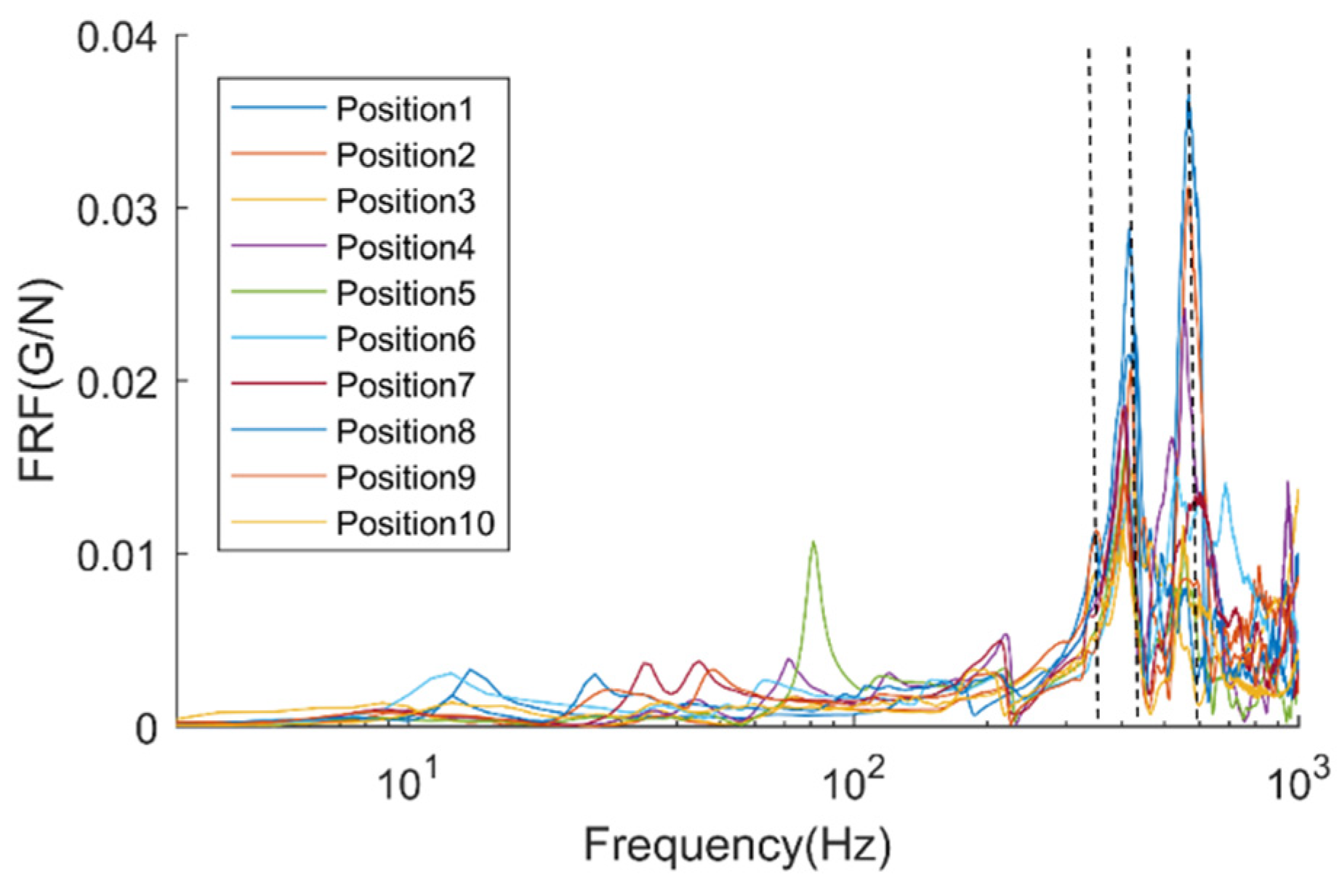
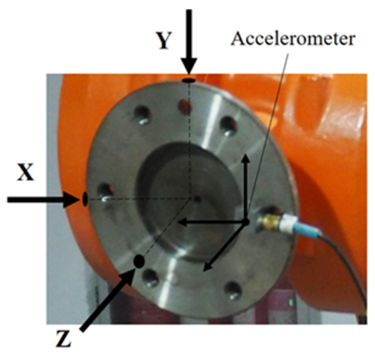
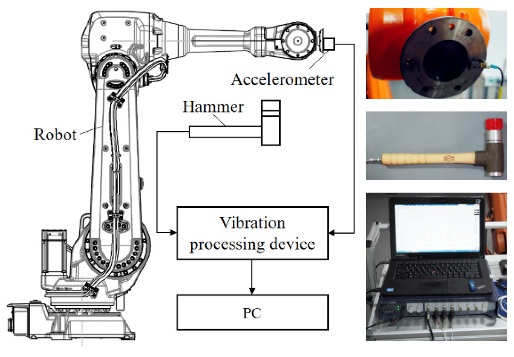
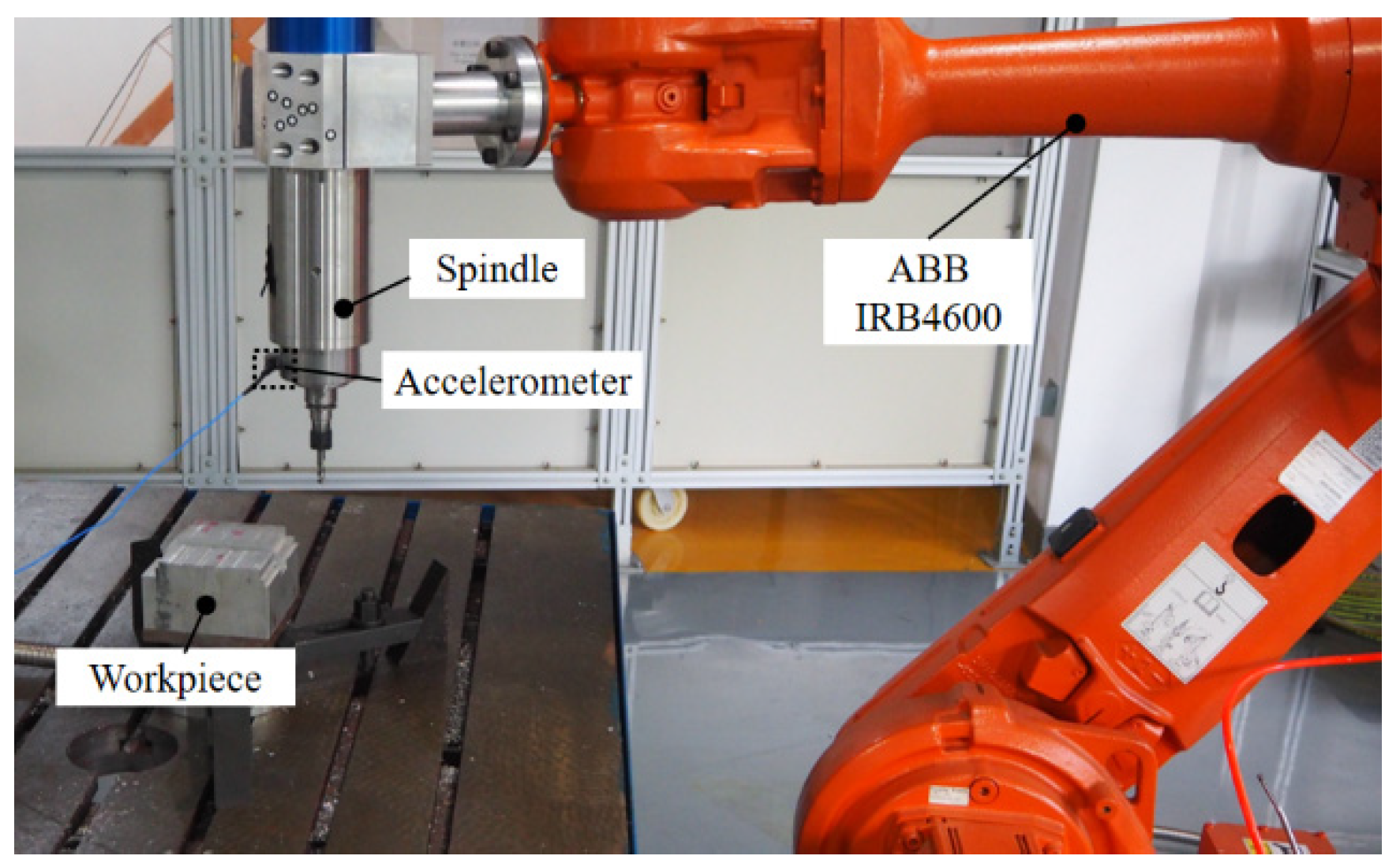
2.1.3. Sample Data Acquisition

Experimental modal test (EMT) is applied so that the natural frequency data of sample configurations can be identified accurately. According to principle of modal test, any element of frequency response function (FRF) can be written as

$$h_{ij}(\omega )={\displaystyle \sum _{k=1}^n\left(\frac{a_{ijk}}{(j\omega -p_k)}+\frac{a_{ijk}^{*}}{(j\omega -p_k^{*})}\right)},$$

(3)

which presents the response of i point caused by the excitation at j point. $a_{ijk}$ and $a_{ijk}^{*}$ are related to mode shapes, their values are depending on relevant combination of excitation and response. $p_{{}_k}$ and $p_k^{*}$ contain the information of natural frequency and damping, which are global characteristics independent of excitation and response combinations. Theoretically, one combination of excitation and response is enough to identify all the natural frequencies, provided the excitation and response points avoid the nodes.

The sample configurations selected by CCD design vary greatly, for the convenience of implementing all the trials in the CCD design, hammer excitation is chosen, and a three-direction accelerometer is fixed on the flange of robot to acquire response signal. In this way, the extra mass brought by EMT device can be negligible as the accelerometer is small and light compared to the robot. Excitations are generated from three directions for each trial, which are corresponding to the three directions of the accelerometer, as shown in Figure 4. Then three FRFs will be obtained for natural frequency identification, avoiding incomplete excitation or excitation on the nodes. Moreover, for each direction, five groups of excitation and response signals are acquired to decrease the signal-to-noise ratio through average algorithm. With FRFs the natural frequencies are preliminarily identified, then complex modal indicating function is used to confirm the accurate values of natural frequencies.

With the ABB IRB4600 industrial robot being the object, a EMT system for sample data acquisition is set up, including a LIXIE hammer, a PCB three-direction accelerometer, an ECON device for vibration signal processing and a PC (as shown in Figure 5). The configuration of robot is adjusted according to the CCD design in turn. All the identified natural frequency information will be used as the sample data to construct a prediction model.

2.2. Prediction Model Construction and Optimization

Because of the serial structure, the relation between configuration and joint angles could not be linear. Thus, Equation (2) is fitted to a general second order equation in this case according to normal engineering application. PLS method is adopted to solve the issues of nonlinear influence and multi-correlation between joint angles in regression equation fitting. Meanwhile, the fitting error caused by the limitation of sample quantity can be remarkably reduced, due to the advantage of PLS method in coping with small sample quantity. In addition, PLS has good interpretability for the terms of regression equation, which can be used as optimization criterion.

2.2.1. PLS Method Fitting Process

The principle of PLS method in multivariate regression fitting is to extract principal components t and u respectively from independent variables X and dependent variables Y while retaining the most correlation, which can be mathematically described as

$$\mathrm{Cov}(\mathit{t},\mathit{u})=\sqrt{\mathrm{Var}(\mathit{t})\mathrm{Var}(\mathit{u})}\mathrm{r}(\mathit{t},\mathit{u})\to \max ,$$

(4)

The process of regression equation fitting by PLS method [27] is briefly introduced as follows.

• Data standardization.
• First principal component calculation.
• Principal component validation.

Current principal component t_h is validated by following indexes:

$$R_Y^2(\mathrm{cum})={\displaystyle \sum _{\mathrm{h}=1}^{\mathrm{m}}{\mathrm{r}}^2(Y,t_{\mathrm{h}})},$$

(5)

$$Q_{\mathrm{h}}^2=1-\frac{S_{SPE,\mathrm{h}}}{S_{SE,\mathrm{h}}},$$

(6)

$$Q_{\mathrm{h}}^2(\mathrm{cum})=1-{\displaystyle \prod _{\mathrm{k}=1}^{\mathrm{h}}\frac{S_{SPE,\mathrm{k}}}{S_{SE,\mathrm{k}}}},$$

(7)

where S_SPE,h is the square sum of prediction error of Y_h−1, S_SE,h is square sum of deviation of Y_h−1.

$R_Y^2(\mathrm{cum})$ indicates the ability of principal component to explain the variability of Y_h−1, and its upper limit value is 1. $Q_{\mathrm{h}}^2$ represents the contribution of t_h to the model. When it is more than (1–0.95)² = 0.0975, t_h has significant effect on prediction model. Meanwhile, $Q_{\mathrm{h}}^2(\mathrm{cum})$ increases, meaning that the comprehensive significance in explaining Y is enhanced.

4.

Subsequent principal components calculation.

The residual matrixes from Step c. are continued to compute new principal components, until t_Q+1 deduces $Q_{\mathrm{h}}^2(\mathrm{cum})$. The principal components before t_Q+1 are validated ones.

5.

Regression equation

$$Y_0=t_1{r}_1^{\mathrm{T}}+t_2{r}_2^{\mathrm{T}}+\dots +t_{\mathrm{Q}}{r}_{\mathrm{Q}}^{\mathrm{T}}+Y_{\mathrm{Q}},$$

(8)

6.

Data reduction.

The final regression equation for prediction can be obtained through the reverse process of data standardization.

2.2.2. Interpretability of PLS Method for Regression Equation

Variable importance in projection (VIP), which indicates the importance of each item in regression equation, is defined as

$${\mathrm{VIP}}_{\mathrm{j}}=\sqrt{\frac{p}{R_Y^2\left(\mathrm{cum}\right)}{\displaystyle \sum _{\mathrm{h}=1}^{\mathrm{m}}{\mathrm{r}}^2\left(Y,t_{\mathrm{h}}\right)}{w}_{\mathrm{hj}}^2},$$

(9)

where w_jh is the jth component of w_h.

The larger VIP_j is, the more important x_j is in constructing Y. The effects of different items can be compared quantitatively through VIP values, so that some redundant items can be rejected to realize regression equation optimization.

2.2.3. Prediction Model Construction

The sample data from Section 2.1.3 is utilized to construct prediction model, taking the first order natural frequency of ABB IRB4600 robot as example.

As mentioned, the general regression equation concludes q₂, q₃, q₄, q₅, and their cross items and square items. The general equation is marked as M. After the second principal component is extracted, validation indicates are shown in

Table 2. Principal component validation of M.

h	${\mathit{R}}_{\mathit{Y}}^2(\mathsf{c}\mathsf{u}\mathsf{m})$	${\mathit{Q}}_{\mathsf{h}}^2$	${\mathit{Q}}_{\mathsf{h}}^2(\mathsf{c}\mathsf{u}\mathsf{m})$
1	0.888	0.639	0.639
2	0.962	−0.171	0.603

. The second principal component deduces $Q_{\mathrm{h}}^2(\mathrm{cum})$, meaning that comprehensive ability is weakened. Though $R_Y^2(\mathrm{cum})$ increases, the second principal component is still abandoned.

2.2.4. Prediction Model Optimization

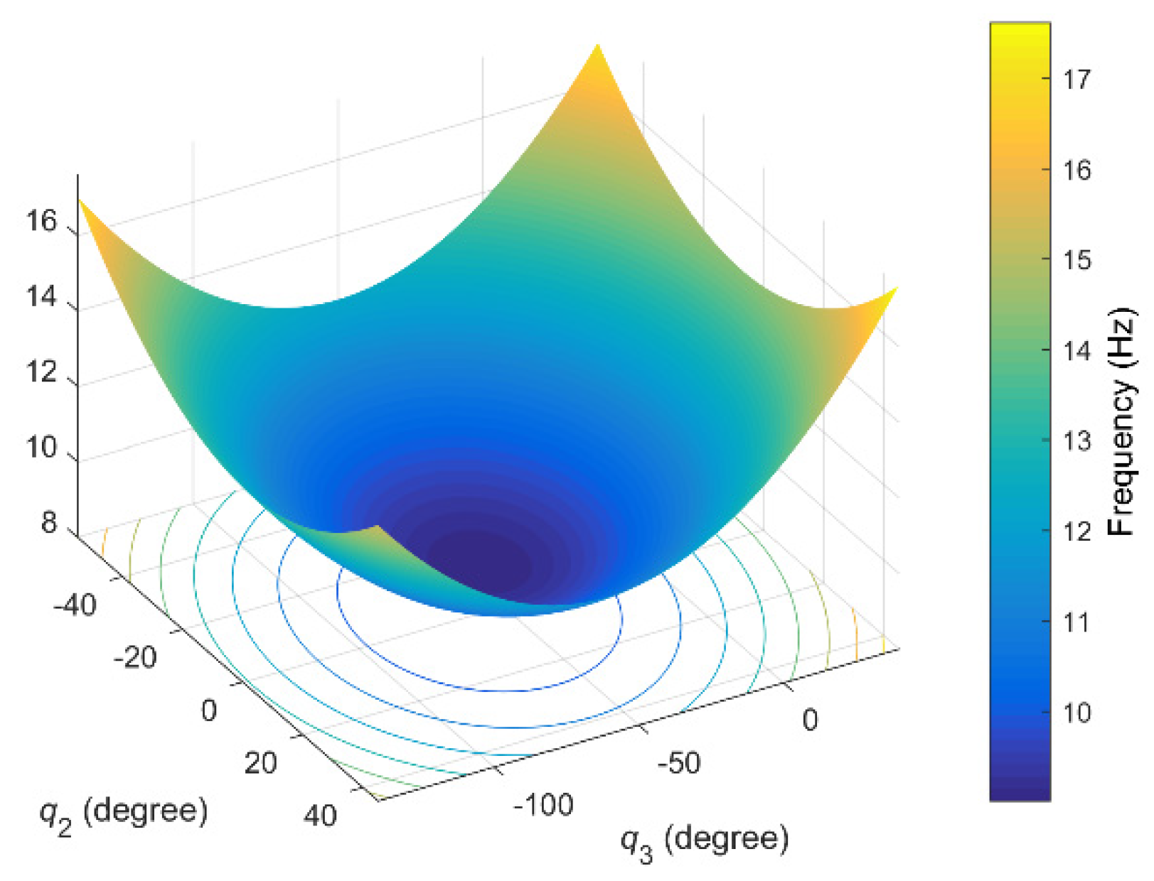
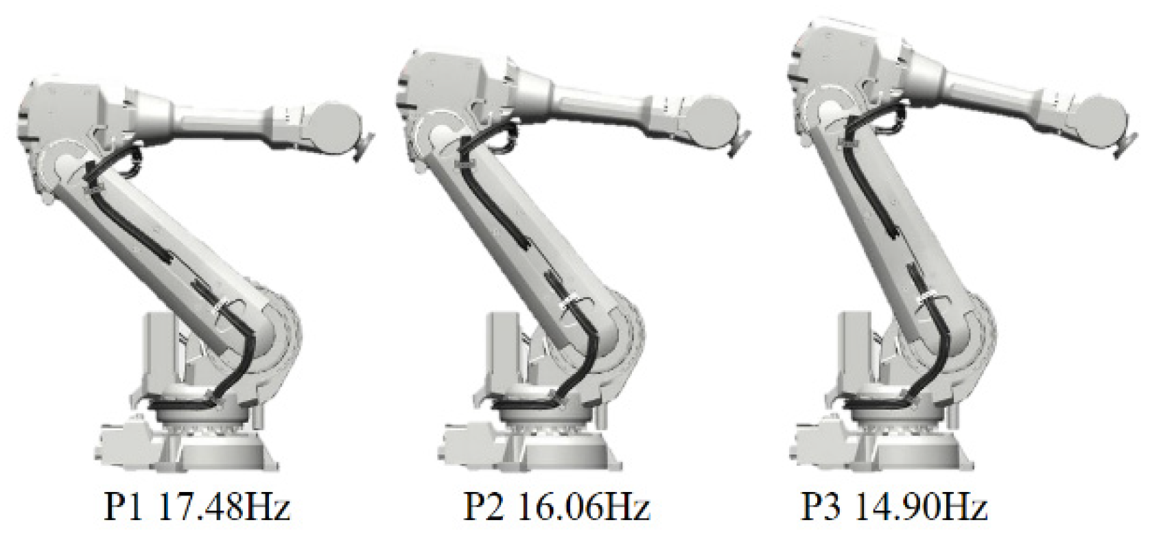
$Q_{\mathrm{h}}^2(\mathrm{cum})$ of M is merely 0.639, which means M is inadequate to represent f_F. To optimize the model, VIP values of items in M is calculated and illustrated in Figure 6.

All the one-degree items should be retained as basic items. All the square items are important enough to stay in the model because of their high VIP values. As VIP values of cross items are relatively low, different combination groups should be tested. A new model M₁ is constructed by cutting off cross items except q₂q₃, because q₂q₃ has the largest VIP value among cross items; meanwhile, q₂ and q₃ are most two important variables according to VIP values. Based on M₁, the other five cross items are added respectively in descending order of their VIP values. The new five models are marked as M₂–M₆. Validation results of above models are shown in

Table 3. Validation results of M₁–M₆.

Model	h	${\mathit{R}}_{\mathit{Y}}^2(\mathsf{c}\mathsf{u}\mathsf{m})$	${\mathit{Q}}_{\mathsf{h}}^2(\mathsf{c}\mathsf{u}\mathsf{m})$
M1	2	0.958	0.776
M2	2	0.960	0.778
M3	2	0.958	0.764
M4	2	0.958	0.762
M5	2	0.958	0.723
M6	2	0.958	0.717

. All the six models are constructed with two principal components. $R_Y^2(\mathrm{cum})$ and $Q_{\mathrm{h}}^2(\mathrm{cum})$ values of the six models are all improved obviously compared to M. M₂, formed by adding q₃q₅ to M₁, has the best $R_Y^2(\mathrm{cum})$ and $Q_{\mathrm{h}}^2(\mathrm{cum})$ values. M₃–M₆, which get lower $R_Y^2(\mathrm{cum})$ and $Q_{\mathrm{h}}^2(\mathrm{cum})$ values compared to M₁, are abandoned.

Based on M₂, four new models are introduced by adding q₂q₄, q₃q₄, q₂q₅, and q₄q₅ in turn. However, the largest $Q_{\mathrm{h}}^2(\mathrm{cum})$ only reaches up to 0.764. All the other combination groups of above four cross items are add to M₂ for test, but none of them can acquire better validation result. Thus, the optimized model is finally confirmed to be M₂. The coefficients of items are listed in

Table 4. Coefficients of items in M and M₂.

Items	Coefficient/M	Coefficient/M2
Constant	1.138 × 101	1.086 × 101
q2	8.746 × 10−3	1.214 × 10−2
q3	5.987 × 10−2	6.611 × 10−2
q4	−7.532 × 10−5	7.873 × 10−4
q5	1.374 × 10−4	−3.785 × 10−3
$q_2^2$	8.821 × 10−4	1.179 × 10−3
$q_3^2$	5.322 × 10−4	5.894 × 10−4
$q_4^2$	−2.464 × 10−5	1.242 × 10−5
$q_5^2$	−1.018 × 10−4	7.342 × 10−5
q2q3	1.171 × 10−4	1.253 × 10−4
q2q4	4.323 × 10−6	-
q2q5	4.224 × 10−5	-
q3q4	−7.206 × 10−6	-
q3q5	−4.939 × 10−5	−5.285 × 10−5
q4q5	1.099 × 10−5	-

together with M.

3. Results

3.1. Prediction Model Verification and Analysis

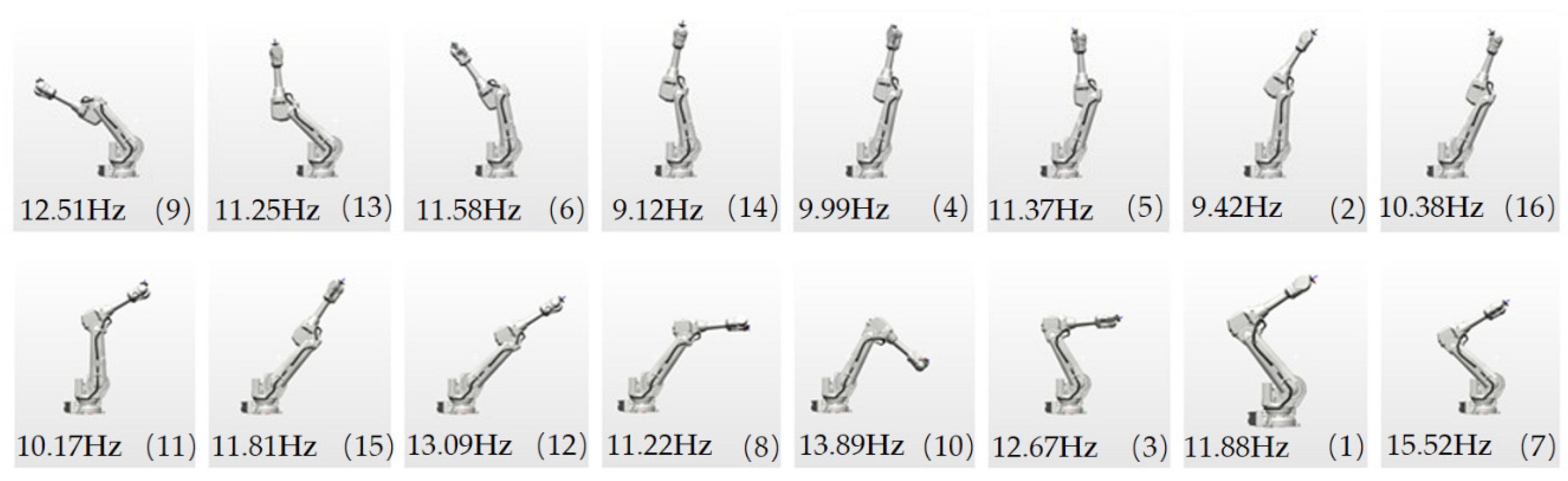
3.1.1. Model Verification with Random Configurations

Sixteen groups of q₂–q₅ values are picked randomly from the variable range defined in Section 2.1.1, through which 16 corresponding robot configurations are defined for model verification. The simulation images of the 16 configurations are reranked by joint angles q₂ and q₃ as shown in Figure 7, and the measured natural frequency is listed in the bottom left corner of each image. The configurations are nearly uniformly distributed in the variable range, which ensures the comprehensiveness of verification objects and rationality of verification result.

The first order natural frequencies of the 16 configurations are obtained by EMT. Then, original model M and optimized model M₂ are utilized to predict the first order natural frequencies. The deviation between prediction value and measured value is defined as prediction error, the details are listed in

Table 5. Prediction error of M.

No.	1	2	3	4	5	6	7	8
Error	0.20	0.36	0.22	0.11	0.22	0.45	1.59	0.26
Relative error %	1.71	3.79	1.76	1.10	1.90	3.88	10.24	2.34
No.	9	10	11	12	13	14	15	16
Error	0.54	1.43	0.87	1.04	1.46	1.78	1.47	0.12
Relative error %	4.34	10.30	8.40	8.27	12.56	19.54	12.39	1.18
Average error	0.76			Average relative error %			6.48

;

Table 6. Prediction error of M₂.

No.	1	2	3	4	5	6	7	8
Error	0.30	0.10	0.19	0.46	0.44	0.44	0.30	0.32
Relative error %	2.51	1.04	1.47	4.55	3.85	3.81	1.92	2.88
No.	9	10	11	12	13	14	15	16
Error	0.51	0.44	0.20	0.51	0.42	0.24	0.11	0.15
Relative error %	4.12	3.14	1.90	4.01	3.56	2.68	0.88	1.48
Average error	0.32			Average relative error %			2.74

.

The average error and average relative error of optimized model M₂ are both much lower than those of original model M. The average relative error of M₂ is less than 5% which brings more reliability. On the other hand, seven high relative errors (more than 5%) which are underlined show up in the prediction process of M, and the maximum error reaches up to 1.78 Hz. While M₂ has no predictions with over 5% relative error, and the maximum error is 0.51 Hz which is acceptable. Obviously, optimized model M₂ has better prediction ability.

A model (M_LS) fitted by least square (LS) method with the same sample data is taken as the contrast. Moreover, the prediction errors are displayed in

Table 7. Prediction error of M_LS.

No.	1	2	3	4	5	6	7	8
Error	0.51	0.45	0.51	0.79	1.16	1.37	0.52	0.86
Relative error %	4.32	4.77	4.01	7.91	10.30	11.81	4.66	7.68
No.	9	10	11	12	13	14	15	16
Error	1.49	0.64	0.55	0.40	1.94	0.36	0.46	0.43
Relative error %	11.92	6.32	4.86	4.38	16.44	3.29	4.43	5.89
Average error	0.78		Average relative error %				7.07

. Average error and average relative error of M_LS are both higher than those of M and M₂, that is, PLS method have better performance in construct prediction model of natural frequency than LS method. In conclusion, model fitted and optimized by PLS method has the best prediction ability.

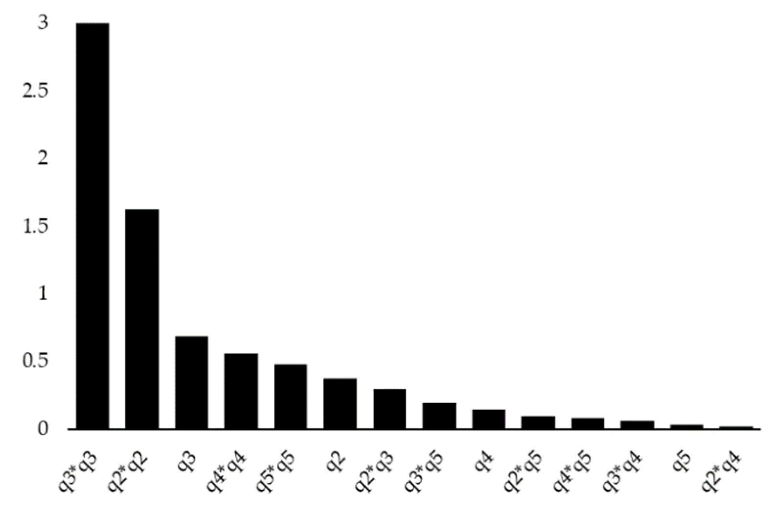
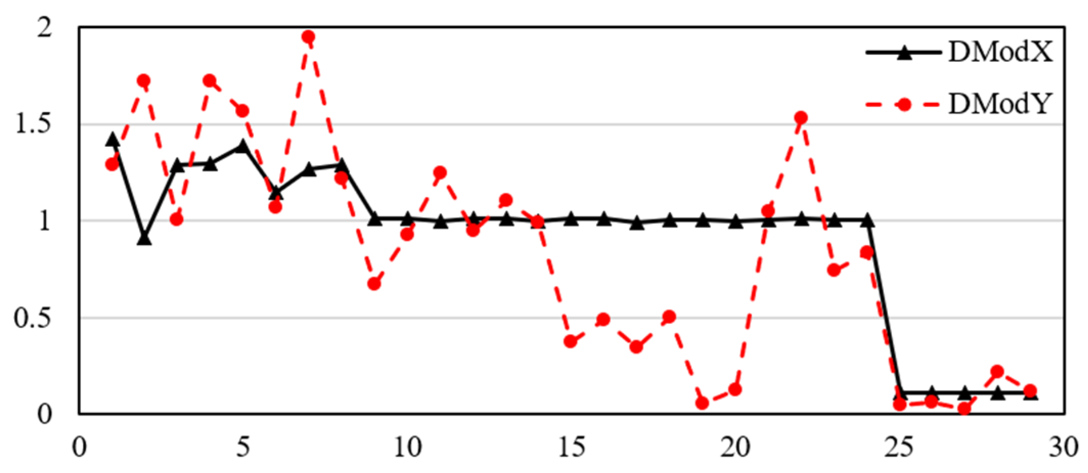
3.1.2. Model Construction Quality Analysis

In PLS method, when model is constructed by principal components, information in the last residual matrix is ignored, causing the error between fitted model and original data. Standardized distance between sample point and model can be used to evaluate the construction quality. (DModX,N)_i or (DModY,N)_i is the ratio of construct quality of the ith sample point and the average construct quality. When the ratio is less than two, the construction for the ith sample point is reasonable. Construction quality of M₂ is shown in Figure 8. (DModX,N)_i and (DModY,N)_i are all less than two, that means the construction of M₂ is rational.

3.2. Method Universality Verification

To testify the universality of the natural frequency prediction method proposed in this paper, it is completely applied to an ABB IRB6400 industrial robot (as shown in Figure 9). Sample data are obtained according to Chapter 2.1 as the structure is similar to IRB4600. PLS is used to fit and optimize the prediction model M₆₄₀₀. In this case, q₂q₄, q₂q₅, and q₄q₅ are abandoned according to VIP values. Validation results can be seen in

Table 8. Validation results of M₆₄₀₀.

h	${\mathit{R}}_{\mathit{Y}}^2(\mathsf{c}\mathsf{u}\mathsf{m})$	${\mathit{Q}}_{\mathsf{h}}^2$	${\mathit{Q}}_{\mathsf{h}}^2(\mathsf{c}\mathsf{u}\mathsf{m})$
1	0.801	0.720	0.720
2	0.952	0.546	0.874

, values of $R_Y^2(\mathrm{cum})$ and $Q_{\mathrm{h}}^2(\mathrm{cum})$ indicate that the fitting is rational. Construction quality is eligible as shown in Figure 10. The result of model verification through random configurations is shown in

Table 9. Prediction error of M₆₄₀₀.

No.	1	2	3	4	5	6	7	8
Error	0.35	0.43	0.13	0.47	0.23	0.23	0.07	0.19
Relative error %	2.94	3.38	1.41	4.16	1.97	1.97	0.44	1.66
No.	9	10	11	12	13	14	15	16
Error	0.15	0.23	0.25	0.61	0.78	0.58	0.35	0.34
Relative error %	1.56	2.05	2.74	4.81	7.19	5.59	3.11	2.78
Average error	0.33			Average relative error %			2.98

, average relative error is merely 2.982%, indicating the good prediction performance.

The two models constructed for two different robots through the method proposed in this paper both own good prediction ability. That is, the universality of the proposed method is testified.

4. Discussion

Once the prediction model of natural frequency is constructed and verified, the prediction result can be used as optimization parameter to improve the machining performance. An application case of the prediction model is explained as follows.

a₂ and a₃ control the two longest links, by which the basic configuration of robot is determined. Through VIP values, items involving q₂ and q₃ are demonstrated to act dominated role in prediction model. a₄ and a₅ decide the direction of robot flange, which affect the configuration less than a₂ and a₃. Taking M₂ for an example, the influence of q₂ and q₃ on natural frequency is specifically studied and illustrated in Figure 11. When q₂ = −55° and q₃ = 40° (P_max), the maximum first order natural frequency is obtained, and the minimum appears when q₂ = −2° and q₃ = −56° (P_min).

Three configurations near P_max, P1 (q₂ = −48°, q₃ = 50°), P2 (q₂ = −38°, q₃ = 45°), and P3 (q₂ = −28°, q₃ = 40°) are chosen for milling test (as shown in Figure 12. The first order natural frequencies decrease in turn from P1 to P3 according to model M₂. The setup of milling test is shown in Figure 13. High speed milling with short and straight path are executed, so that robot configuration can be ignored in one milling path. Milling parameters are as follows: the spindle rotation frequency is 800 Hz, f is 2.4 mm/s, a_e is 1 mm, and a_p is 4 mm. Acceleration signals and milled surface are analyzed.

Milling acceleration signals are treated with short-time fourier transform (STFT), spectrograms of the range 5–100 Hz are displayed in Figure 14. For all three configurations, several peaks are conspicuous around 50–90 Hz during the whole milling process. In low frequency stage, a peak about 16 Hz can be found in P2 and a 15 Hz peak for P3, which are corresponding to their predicted natural frequencies. That no conspicuous can be found in P1, may because the certain frequency is not significantly impacted by the milling parameters.

As for the milled surface, an obvious tool recession appears at P3, as shown in the red frame in Figure 15, while the situations are better in at P1 and P2. In addition, the quality of milled surfaces at P3 is the poorest compared with P1 and P2, and the vibration phenomenon on milled surface is getting severer from P1 to P3, indicating that configuration with higher first order frequency may lead to better milling performance, as mentioned in [20]. Whether there exits practical relevance between the value of natural frequency and machining performance can be a further research topic to develop more application of natural frequency prediction.

5. Conclusions

It is impossible to measure all the natural frequency information of the whole robot workspace, but the information is vital in improving robot milling performance. In view of that, a method to predict the natural frequency is proposed in this paper. The core content of the method proposed is to construct a prediction model with sample configurations, which takes joint angles as input variables. Two insignificant variables q₁ and q₆ are abandoned and workspace is limited for practicability. Considering the nonlinear influence of joint angles on natural frequency, CCD method is used to select sample configurations from limited variable range, and EMT is applied to acquire the sample data of the example robot. Several models are fitted through the sample data. The model validation procedure proves that the model fitted and optimized by PLS method has the best prediction ability. Then the method proposed is applied completely onto another robot for universality verification, and the prediction performance turns out to be outstanding. Thus, this method can be applied on any 6R machining industrial robot to evaluate its natural frequency distribution, which can be used for in machining performance improvement.

References

1. International Federation of Robotics. Available online: https://www.ifr.org/# (accessed on 1 October 2020).
2. Chen, Y.; Dong, F. Robot machining: Recent development and future research issues. Int. J. Adv. Manuf. Technol. 2013, 66, 1489–1497. [Google Scholar] [CrossRef] [Green Version]
3. Kazerooni, H.; Bausch, J.J.; Kramer, B.M. An Approach to Automated Deburring by Robot Manipulators. J. Dyn. Syst. Meas. Control. 1986, 108, 354–359. [Google Scholar] [CrossRef]
4. Vergeest, J.S.; Tangelder, J.W. Robot machines rapid prototype. Ind. Robot. Int. J. 1996, 23, 17–20. [Google Scholar] [CrossRef]
5. Zieliński, C.; Mianowski, K.; Nazarczuk, K.; Szynkiewicz, W. A prototype robot for polishing and milling large objects. Ind. Robot. Int. J. 2003, 30, 67–76. [Google Scholar] [CrossRef]
6. Sun, L.; Liang, F.; Fang, L. Design and performance analysis of an industrial robot arm for robotic drilling process. Ind. Robot. Int. J. 2019, 46, 7–16. [Google Scholar] [CrossRef]
7. Guo, Y.; Dong, H.; Wang, G.; Ke, Y. A robotic boring system for intersection holes in aircraft assembly. Ind. Robot. Int. J. 2018, 45, 328–336. [Google Scholar] [CrossRef]
8. Matsuoka, S.-I.; Shimizu, K.; Yamazaki, N.; Oki, Y. High-speed end milling of an articulated robot and its characteristics. J. Mater. Process. Technol. 1999, 95, 83–89. [Google Scholar] [CrossRef]
9. Brunete, A.; Gambao, E.; Koskinen, J.; Heikkilä, T.; Kaldestad, K.B.; Tyapin, I.; Hovland, G.; Surdilovic, D.; Hernando, M.; Bottero, A.; et al. Hard material small-batch industrial machining robot. Robot. Comput. Integr. Manuf. 2018, 54, 185–199. [Google Scholar] [CrossRef]
10. Dong, X.; Zhang, W.; Sun, J. The estimation of cutting force coefficients in milling of thin-walled parts using cutter with different tooth radii. Proc. Inst. Mech. Eng. Part B J. Eng. Manuf. 2014, 230, 194–199. [Google Scholar] [CrossRef] [Green Version]
11. Dong, X.; Zhang, W. Chatter suppression analysis in milling process with variable spindle speed based on the reconstructed semi-discretization method. Int. J. Adv. Manuf. Technol. 2019, 105, 2021–2037. [Google Scholar] [CrossRef]
12. Dong, X.; Qiu, Z. Stability analysis in milling process based on updated numerical integration method. Mech. Syst. Signal Process. 2020, 137, 106435. [Google Scholar] [CrossRef]
13. Pan, Z.; Zhang, H.; Zhu, Z.; Wang, J. Chatter analysis of robotic machining process. J. Mater. Process. Technol. 2006, 173, 301–309. [Google Scholar] [CrossRef]
14. Guo, Y.; Dong, H.; Ke, Y. Stiffness-oriented posture optimization in robotic machining applications. Robot. Comput. Integr. Manuf. 2015, 35, 69–76. [Google Scholar] [CrossRef]
15. Lin, Y.; Zhao, H.; Ding, H. Spindle configuration analysis and optimization considering the deformation in robotic machining applications. Robot. Comput. Integr. Manuf. 2018, 54, 83–95. [Google Scholar] [CrossRef]
16. Chen, C.; Peng, F.; Yan, R.; Li, Y.; Wei, D.; Fan, Z.; Tang, X.; Zhu, Z. Stiffness performance index based posture and feed orientation optimization in robotic milling process. Robot. Comput. Integr. Manuf. 2019, 55, 29–40. [Google Scholar] [CrossRef]
17. Xiong, G.; Ding, Y.; Zhu, L.-M. Stiffness-based pose optimization of an industrial robot for five-axis milling. Robot. Comput. Integr. Manuf. 2019, 55, 19–28. [Google Scholar] [CrossRef]
18. Zaeh, M.F.; Roesch, O. Improvement of the Static and Dynamic Behavior of a Milling Robot. Mini Special Issue on Virtual Manufacturing. Int. J. Autom. Technol. 2015, 9, 129–133. [Google Scholar] [CrossRef]
19. Mejri, S.; Gagnol, V.; Le, T.-P.; Sabourin, L.; Ray, P.; Paultre, P. Dynamic characterization of machining robot and stability analysis. Int. J. Adv. Manuf. Technol. 2015, 82, 351–359. [Google Scholar] [CrossRef]
20. Bisu, C.; Cherif, M.; Gerard, A.; K’Nevez, J.Y. Dynamic Behavior Analysis for a Six Axis Industrial Machining Robot. Adv. Mater. Res. 2011, 423, 65–76. [Google Scholar] [CrossRef] [Green Version]
21. Mousavi, S.; Gagnol, V.; Bouzgarrou, B.C.; Ray, P. Model-based stability prediction of a machining robot. In New Advances in Mechanisms, Mechanical Transmissions and Robotics; Springer: Cham, Switzerland, 2017; pp. 379–387. [Google Scholar]
22. Karim, A.; Hitzer, J.; Lechler, A.; Verl, A. Analysis of the dynamic behavior of a six-axis industrial robot within the entire workspace in respect of machining tasks. In Proceedings of the 2017 IEEE International Conference on Advanced Intelligent Mechatronics (AIM), Munich, Germany, 3–7 July 2017; pp. 670–675. [Google Scholar]
23. Glogowski, P.; Rieger, M.; Bin Sun, J.; Kuhlenkötter, B. Natural Frequency Analysis in the Workspace of a Six-Axis Industrial Robot Using Design of Experiments. Adv. Mater. Res. 2016, 1140, 345–352. [Google Scholar] [CrossRef]
24. Guo, Y.; Dong, H.; Wang, G.; Ke, Y. Vibration analysis and suppression in robotic boring process. Int. J. Mach. Tools Manuf. 2016, 101, 102–110. [Google Scholar] [CrossRef]
25. Cordes, M.; Hintze, W.; Altintas, Y. Chatter stability in robotic milling. Robot. Comput. Integr. Manuf. 2019, 55, 11–18. [Google Scholar] [CrossRef]
26. Simões, J.A.; Coole, T.; Cheshire, D.; Pires, A.M. Analysis of multi-axis milling in an anthropomorphic robot, using the design of experiments methodology. J. Mater. Process. Technol. 2003, 135, 235–241. [Google Scholar] [CrossRef]
27. Wang, H.; Wu, Z.; Meng, J. Partial Least-Square Regression—Linear and Nonlinear Methods; National Defense Industry Press: Beijing, China, 2006; pp. 97–123. [Google Scholar]
Figure 1. Frequency Response Functions of different robot configurations.
Applsci 10 08138 g001
Figure 2. Prediction method of robot natural frequency.
Applsci 10 08138 g002
Figure 3. Partial variable range.
Applsci 10 08138 g003
Figure 4. Directions of accelerometer and excitations.
Applsci 10 08138 g004
Figure 5. The setup of experimental modal test (EMT) system.
Applsci 10 08138 g005
Figure 6. VIP values of items in M.
Applsci 10 08138 g006
Figure 7. Random configurations for model verification.
Applsci 10 08138 g007
Figure 8. Construction quality of M2.
Applsci 10 08138 g008
Figure 9. ABB IRB6400 industrial robot.
Applsci 10 08138 g009
Figure 10. Construction quality of M6400.
Applsci 10 08138 g010
Figure 11. Variation of natural frequency with q2 and q3.
Applsci 10 08138 g011
Figure 12. Chosen robot configurations for milling test.
Applsci 10 08138 g012
Figure 13. Milling test system setup.
Applsci 10 08138 g013
Figure 14. Short-time fourier transform (STFT) of vibration signals of P1–P3.
Applsci 10 08138 g014
Figure 15. Milled surfaces of P1–P3.
Applsci 10 08138 g015