A Machine Learning Model for Predicting Noise Limits of Motor Vehicles in UNECE R51 Regulations

Abstract

It is vital to greatly reduce traffic noises emitted by motor vehicles during accelerating through determining limit values of noises and further improve technical specifications and comforts of these automobiles for automotive manufacturers. The United Nations Economic Commission for Europe (UNECE) R51 regulations define the noise limits for all vehicle categories, which are kept updating, and these noise limits are implemented by governments all over the world; however, the automobile manufactures need to estimate future values of noise limits for developing their next-generation vehicles. In this study, a machine learning model using the back-propagation neural network (BPNN) approach is developed to determine noise limits of a vehicle during accelerating by using historic data and predict its noise limits for future revisions of the UNECE R51 regulations. The proposed prediction model adopts the Levenberg-Marquardt algorithm which can automatically adapt its learning rate to train the model with input data, and at the same time randomly select the validation data and test data to verify the correlation and determine the accuracy of the prediction results. To showcase the proposed prediction model, acceleration noise limits from six historic data are used for training the model, and the noise limits at the seventh version can be predicted and validated. As the results achieve a required accuracy, vehicle noise limits in the next revision as the future eighth version can be predicted based on these data. It can be found that the obtained prediction results are much close to those noise limits defined in current regulations and negative error ratios are reduced significantly, compared to those values obtained using a quadratic regression model. As a result, the proposed BPNN model can predict future noise limits for the next revision of the UNECE R51automotive noise limit regulations.

1. Introduction

Traffic noises, mainly generated by motor vehicle, aircraft, train, ship etc. during operation, refer to those unwanted sounds that hinder people’s normal life and work. The motor vehicle noises are much severe when motor vehicles travel on main roads in municipal areas. These noises are unstable and random, and they greatly contribute sound pollutions to many audiences in urban regions. Their sound pressure levels keep changing with time and correlating with multiple factors, e.g., road type, vehicle type, vehicle number, and operating status of motor vehicles. The noise pollutions of motor vehicles are very large, and they can cause hearing reduction and damage of audiences and generate significant impacts on audiences’ emotion, rest and physical health, and interrupt their conversation and communication [1,2]. Therefore, it is vital to investigate the motor vehicle noises during operating and formulate and promulgate noise limits that fulfil the requirements regulated in automotive noise limits regulations.

The automobile manufacturers are always pursuing to lower the noises emitted by their vehicles to advance the automobile technology and then improve the comfort of urban life, and continuously reducing adverse effects of noise on humans. Automobiles manufactured should follow the requirements according to local regulations and standards. These regulations and standards include International Organization for Standardization (ISO) standards for automobile noise regulations, American Society of Automotive Engineers (SAE) standards, Japanese regulations, United Nations Economic Commission for Europe (UNECE) regulations, etc. UNECE regulations are one of the most influential automotive technical regulations and certification systems in the world today [3]. In this study, the UNECE regulations were focused, which are based on the UN/ECE/WP29 “1958 Agreement” framework, and automobile products approved by the UNECE regulations are mutually recognised among parties to the “1958 Agreement”. The current regulations of UNECE regulations concerning automobile noise are UNECE R51.03 “Uniform Provisions Concerning the Approval of Motor Vehicles Having a Least Four Wheels with Regard to their Sound Emissions”, which came into effects on 16 October 1995, and the current revised version came into effects on 5 February 2016. It stipulates the measurement method on external noises of the vehicle when the vehicle accelerates, and external noises emitted by stationary road vehicles, respectively. It also specifies the limits of noise emission with the vehicle when it accelerates, as shown in

Table 1. Limits of motor vehicle noises during acceleration regarding noise emissions in United Nations Economic Commission for Europe (UNECE) regulations.

UNECE Regulations		Limits of Motor Vehicle During Acceleration (dB(A))
Categories of vehicles	Regulation No.	R9/00	R51/00	R51/01	R51/02	R51/03I	R51/03II	R51/03III
	Year	1969	1982	1988	2005	2016	2020	2024
	Revision No.	1	2	3	4	5	6	7
M1	PMR ≤ 120	82	80	77	74	72	70	68
	120 < PMR ≤ 160	82	80	77	74	73	71	69
	PMR > 160	82	80	77	74	75	73	71
M2	M ≤ 2.5 t	84	81	77	74	72	70	69
	2.5 t < M ≤ 3.5 t	84	81	77	74	74	72	71
	M > 3.5 t; Pn ≤ 135 kW	89	82	80	78	75	73	72
	M > 3.5 t; Pn > 135 kW	91	85	83	80	75	74	72
M3	Pn ≤ 150 kW	89	82	80	78	76	74	73
	150 kW < Pn ≤ 250 kW	91	85	83	80	78	77	76
	Pn > 250 kW	91	85	83	80	80	78	77
N1	M ≤ 2.5 t	84	81	78	76	72	71	69
	M > 2.5 t	84	81	79	77	74	73	71
N2	Pn ≤135 kW	89	86	83	78	77	75	74
	Pn > 135 kW	89	86	84	80	78	76	75
N3	Pn ≤ 150 kW	89	86	83	78	79	77	76
	150 kW < Pn ≤ 250 kW	92	88	84	80	81	79	77
	Pn > 250 kW	92	88	84	80	82	81	79

Note: PMR, power-to-mass ratio; M, Mass; P_n, Power; M, Vehicles having at least four wheels and used for the carriage of passengers (e.g., standard car with 2, 3, 4 doors). M1: Vehicles used for the carriage of passengers, comprising not more than eight seats in addition to the driver’s seat = 9. (Larger Than Standard Car, e.g., London Cab/E7 Type Vehicle 8 seat + Driver seat.). M2: Vehicles used for the carriage of passengers, comprising more than eight seats in addition to the driver’s seat, and having a maximum mass not exceeding 5 tons. (Bus). M3: Vehicles used for the carriage of passengers, comprising more than eight seats in addition to the driver’s seat, and having a maximum mass exceeding 5 tons. (Bus). N Power-driven vehicles that have at least four wheels and used for the carriage of goods. N1: Vehicles used for the carriage of goods and having a maximum mass not exceeding 3.5 tons. (Pick-up Truck, Van). N2: Vehicles used for the carriage of goods and having a maximum mass exceeding 3.5 tons, but not exceeding 12 tons. (Commercial Truck). N3: Vehicles used for the carriage of goods and having a maximum mass exceeding 12 tons. (Commercial Truck).

.

According to Table 1, the revisions of UNECE R51 regulations are becoming much frequently, from more than 10 years to recently 4 years as a cycle. It is challenging for the automotive industry to improve vehicle designs to fully fulfil the requirements.

There were a certain number of researchers working on the investigation of automotive vehicle exterior noises. Sottek et al. [4] developed a hybrid model for the calculation of binaural vehicle exterior noise to simulate the situation of traffic noise in cities and suburbs, and the model used recordings of the main excitation signals (exhaust system, intake, engine, tires) and binaural filters describing the transfer paths from the sources to an artificial head standing at a distance of several meters outside the vehicle. McBride Granda [5] proposed a contact model to predict the tyre-pavement interaction noise for the pavement and the tyre, which was identified as main sources of vehicle exterior noise. In this work, a precise tyre model was created considering orthotropic material properties and described interactions between belt and sidewalls, inflation pressure and rotation of the tyre, etc. Sarkan et al. [6] carried out a practical measurement on exterior noise of road vehicle in motion and evaluated exterior noise reductions at various levels of engine speed. Phan et al. [7] used an unsteady computation fluid dynamics (CFD) simulation to predict vehicle exterior wind noise and obtain quantitative information about acoustic power of exterior wind noise in vehicle, and indicated the location of the dominant source of exterior wind noise. Baudet et al. [8] presented a numerical process on the dynamic coupling of exterior parts of a vehicle to determine flow and pressure around the vehicle and optimised the vehicle shape for reducing exterior wind noise. Nygren et al. [9] aimed to provide a comparison of the total environmental impact from exterior noise exposure and energy demand and correlated effects of exterior noise-level and energy demand along different travel routes. Kerber [10] proposed a psycho-acoustic test to establish a relationship between the critical distances and the real reaction times needed to respond to the vehicle exterior noise of various approaching vehicles, and achieved a sound compromise between the conflicting objectives of pedestrian safety and vehicle exterior noise-level reduction. Tousignant et al. [11] used exterior transfer path approach to evaluate the sensitivity of variables, such as speaker location, noise source routing, exterior noise transfer functions, and sound source design to achieve the required levels and directivity, while minimising overall exterior noise intrusion.

Artificial neural networks were also utilised by researchers to investigate road traffic noises. Qi et al. [12] identified a generalised loss of mean absolute error between predicted and expected feature vectors in Deep Neural Networks (DNN), which is upper bounded by the sum of an approximation error, and estimation error, and an optimisation error. They performed a set of images denoising, and speech enhancement experiments as a showcase, and the upper bounds for DNN based vector-to-vector regression were found valid. Nourani et al. [13] used an emotional artificial neural network to model road traffic noise. They designed a sensitive analysis experiment and ranked the vitality of input parameters in the road traffic noise level in two places, followed by the number of cars, medium vehicles, heavy vehicles, average speed, and percentage of heavy vehicles, respectively. Jiménez-Romero, et al. [14] proposed two multitask artificial neural network (ANN) models to model acoustic behaviours of an induction motor as a power system of the vehicle. They demonstrated that multitask ANN models are effective for extracting common characteristics from multiple tasks and modelling the noise and acoustic quality of an induction motor. Lu and Wang [15] developed an ANN prediction model for automobile interior noise based on an extension data mining (EDM) algorithm considering basic vehicle parameters, such as the total number of engine valves, engine torque, vehicle, and vehicle speed as inputs of the model. Çelebi et al. [16] used an ANN to predict the sound and vibration of a diesel engine. This proposed ANN model can be used to predict vibration and sound pressure level (SPL) in an acceptable accuracy, which used a Levenberg-Marquardt training algorithm providing more accurate predictions than the regression approach. The number of hidden layers in an ANN model is usually chosen by using the trial-and-error method for stability and accuracy. Huang, et al. [17] used ANN for modelling traffic noise which generates around high-rise building along the urban expressway. In their research, multi-layer perception (MLP) was used to train the network, and they found the minimum number of hidden layers is 3 by using the trial-and-error method. Steinbach and Altinsoy [18] used ANN to conduct annoyance evaluations of electric vehicle noise generated by single-car pass-by situation with a constant speed. The proposed ANN models were able to save time, money and resources comparing with linear regression models based on psycho-acoustic parameter.

Previous research mainly covered vehicle noise prediction, simulation, and co-relation between noise-level and pedestrian safety for design improvement and noise control. Noise limits of various categories of vehicles defined in UNECE R51 have important influences on noise control of automotive vehicles and automotive design. However, limit values of vehicle noises defined in current standards and regulations need to be reviewed because a newly launched vehicle with improved noise controls may not comply with these UNECE regulations. From automotive manufacturers’ points of view, the future revisions of these noise limits are vital for improving their vehicle design, and the estimation of them would be very helpful to avoid being out-of-date of their products in the aspect of noise control. Therefore, in this study, by using the data collected on vehicle noise limits in current regulations, the machine learning model-BPNN (back-propagation neural network) is developed to determine noise limits of a vehicle by using time series data and to predict the vehicle’s acceleration noise limits for next revision of UNECE R51. The proposed prediction model adopts the Levenberg-Marquardt algorithm which can automatically adapt its learning rate to train the model with input data, and at the same time randomly select the validation data and test data to verify the correlation and determine the accuracy of the prediction results. As a showcase to use the proposed prediction model, historic acceleration noise limits available from six versions of UNECE R51 are used for training the model, and then the acceleration noise limits for its incoming seventh version can be predicted and validated.

2. Artificial Neural Network

Neural networks were fully-connected three layers networks with two biases, trained with simple, unadorned back-propagation in the literature [19,20]. In 1986, Rumelhart and McCelland proposed the back-propagation (BP) learning algorithm [21], based on the multi-layer neural network model. The BP algorithm solves the learning problem of multi-layer neural networks and proves the learning and computing capabilities of multi-layer neural networks [22].

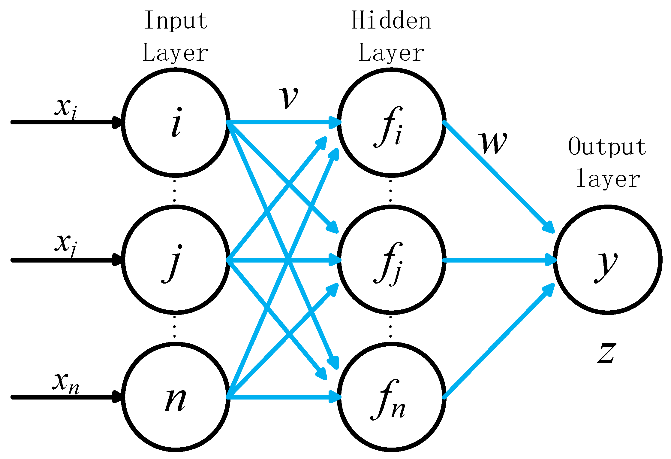
2.1. Principles and Basic Architecture

The BPNN can learn and store a large number of input-output pattern mapping relationships without revealing mathematical equations describing such mapping relationships in advance. The topological structure of the BPNN model has three layers, which include an input layer, hidden layer, and output layer. Its network architecture is shown in Figure 1. The circle in Figure 1 represents the artificial neuron. Note that $x_i,x_j$and $x_n$ represents the inputs of the artificial neural network and they are the components of the vector $x$; $y$ represents the actual output of the artificial neural network; and $z$ represents the expected output of the artificial neural network. The integers $i,j,n$ are the data pre-processing units of the neural network, and $f_i,f_j,f_n$ are the activation functions, which are the components of the vector $f$ as the adder or the multiplier. $v$ is the connection weight vector or threshold vector between the input layer and the hidden layer, and $w$ is the connection weight vector or threshold vector between the hidden layer and the output layer, respectively. There is no connection between the same layer of the network and full unidirectional interconnection between different layers. If the layers of input and the output were proposed, the relationship between the input and the output will be:

$$y=f(vx+w)$$

(1)

The activation functions must be a quasi-linear one which is continuous, derivable, and monotonously incremental. It can be chosen as following Sigmoid function:

$$f(x)=\frac{1}{1+e^{-x}}$$

(2)

A sigmoid function is a bounded, differentiable, real function that is defined for all real input values and has a non-negative derivative at each point [23] and exactly one inflexion point.

2.2. Neural Network Learning

The learning problem is formulated in terms of the minimisation of mean squared errors (MSE). It is a function which can be expressed as

$$MSE=\frac{1}{n}{\displaystyle \sum _i^n{(y_i-{\widehat{y}}_i)}^2}$$

(3)

where $y_i$ are observed values of the variable being predicted and ${\widehat{y}}_i$ are predicted values, respectively.

The performance function is usually used to evaluate how a neural network fits the data set and prevent overfitting by controlling enough complexity of the neural network. The learning of the BPNN includes two stages: The first stage is to learn the input samples and calculate the output of each neuron backward from the first layer of the network through the set network structure and the weight of the previous iteration. The second stage is to modify the weight vector. Its process is to calculate the result of the change of weight vector on the total error from the last layer, and then modify the weight vector according to the process of minimisation of MSE. These two processes repeatedly alternate until the total error convergence.

3. BPNN Model for Noise Limits Prediction during Vehicle Acceleration

BPNN is mainly used in regression prediction (fitting, data processing analysis, object prediction, control, etc.), classification recognition (for type division, pattern recognition). In terms of application. In this study, based on specific data available on vehicle noise limits, the BPNN model is developed and used to self-learn and generate the data to predict the vehicle’s acceleration noise limits, which are helpful for next revision of UNECE R51.

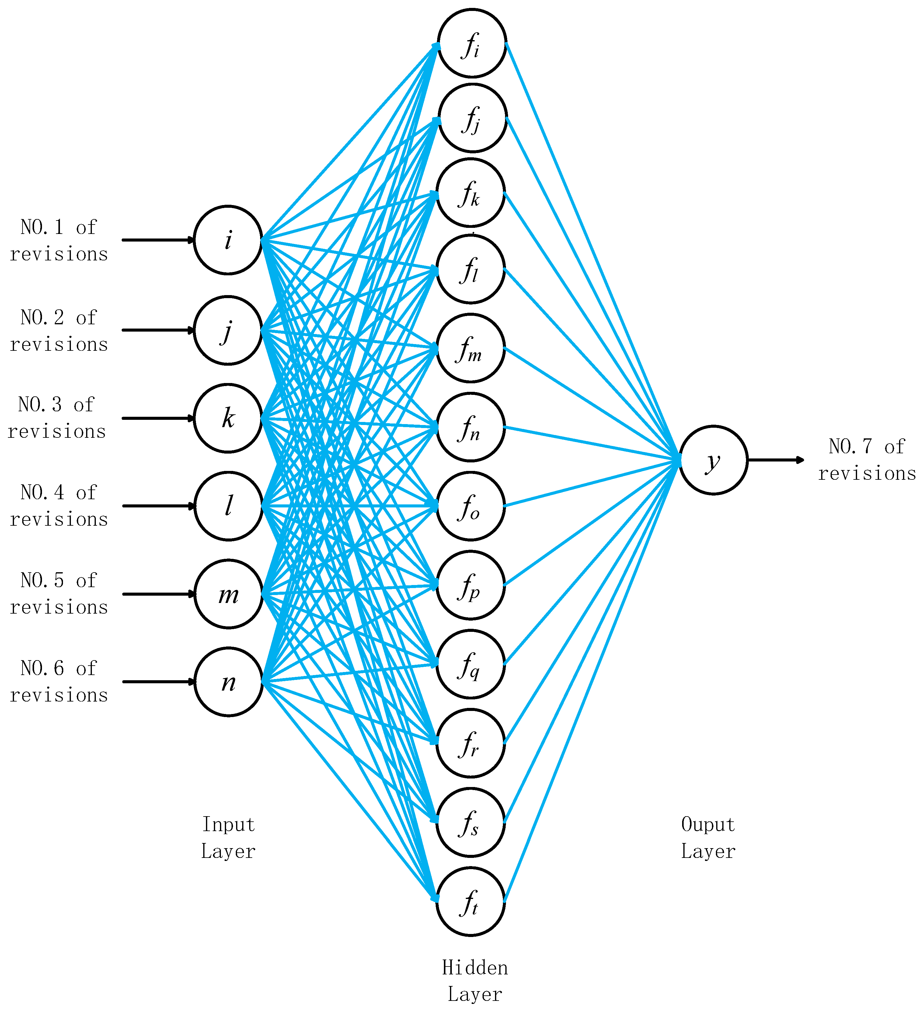
3.1. Architecture of the Proposed BPNN Model

3.1.1. Data Normalisation and Classification

The accuracy of a BPNN model relies on the selection of input data and the preparation of training samples. For data selection, the representativeness of the samples and the elimination of contradictory samples should be considered, and then the data need to be normalised. In MATLAB, a built-in normalisation function is available, which can easily rigidise and convert the data into a data mapping between [−1, 1] or [0, 1]. Data are classified into three sets: (a) Training data, (b) validation data, and (c) test data. The training data are used for neural network learning and training. The validation data are used to confirm that the sample error of the validation data does not fall or rise after six consecutive iterations. The network training is terminated. It can effectively avoid overfitting, that is, in learning and training, the neural network achieves a very high approximation accuracy for the learning samples. However, for non-learning samples, there is a possibility of singular phenomena [12]. For example, generated approximation errors on the outputs by using the validation data decreases first with the number of training times, but then rises. Therefore, these are also used to measure network generalisation, and to halt training when the generalisation has no further improvements. The test data, as the third set, have no effects on training and so provide an independent measure of network performance during and after training.

3.1.2. Development of Back-Propagation Neural Network

The hidden unit in the BPNN can be set freely according to the objective of this study. A three-layer network can facilitate continuous functions with an acceptable precision set by a developer [24,25]. In this study, according to the characteristics of the vehicle acceleration noise limits analysed above, the three-layer neural network is established, that is, the input layer, the hidden layer (only a single-layer neural unit), and the output layer. In the UNECE R51 regulations, the vehicle acceleration noise limits were revised seven times so far for six major vehicle categories. If the noise limits in the regulations is assumed as a function of time to describe its variations, new revised limits can be predicted based on past known limits. Therefore, in the BPNN model, the data of the previous six noise limits revisions can be extracted from all revisions as input data, and the output is the newly revised value, which would be the seventh minor revision value. Then the mapping between input data and output data can be conducted via the BPNN self-learning until the minimum root mean square value is achieved. There is no scientific model or formula to determine the number of hidden layer units. In this study, a trial-and-error method was used to determine the number of hidden layers, which was selected by the value of MSE results from training data, validation data and test data. The maximum MSE is lower than 2.0 from hidden layer units 12 to 24, while the maximum MSE is higher than 2.0 from hidden layer units 6 to 12, as shown in

Table 2. Mean squared errors (MSE) and regression values with a different number of hidden layers.

Number of Hidden Layers	Training Data		Validation Data		Test Data
	MSE	Regression Values	MSE	Regression Values	MSE	Regression Values
6	0.601	0.996	0.340	0.950	2.08	0.999
7	9.61 × 10−3	0.999	1.39	0.905	2.26	0.899
8	3.92 × 10−3	0.999	7.27 × 10−2	0.996	2.36	0.976
9	0.167	0.992	3.92	0.772	1.28	0.999
10	0.127	0.995	2.88	0.965	2.25	0.945
11	4.74 × 10−2	0.999	2.22	−0.694	2.39	−0.761
12	3.64 × 10−2	0.999	1.20	0.995	1.18	0.999
13	9.61 × 10−2	0.995	1.23	0.915	0.536	0.991
14	1.86 × 10−7	0.999	0.178	0.999	1.12	0.969
15	0.133	0.998	0.785	0.999	1.77	0.997
16	0.1.0040	0.993	8.99×10−2	0.997	1.45	0.974
17	9.99 × 10−4	0.999	0.439	0.999	1.25	0.997
18	2.97 × 10−8	0.999	0.869	0.927	1.44	0.946
19	5.03 × 10−5	0.999	1.09	0.992	0.899	0.981
20	9.77 × 10−12	0.999	1.49	0.994	1.49	0.976
21	0.219	0.994	0.957	0.952	1.99	0.997
22	0.857	0.971	1.31	0.998	1.16	0.999
23	1.32 × 10−4	0.999	0.619	0.998	1.21	0.995
24	0.277	0.998	0.488	0.999	1.07	0.999

(highlighted with grey colour), so the number of hidden layer neural units is 12, due to the minima of hidden layers. Hereby, the architecture of the BPNN model was proposed as 6–12–1 (6 inputs, 12 hidden layer units, and 1 output), as depicted in Figure 2.

3.2. Training of the Neural Networks

Before conducting the training, the parameters of the BPNN need to be set and initialised. The training target accuracy was set to 0.001. Levenberg-Marquardt algorithm with an adaptive learning rate were selected for the training function. The Levenberg-Marquardt algorithm combines two numerical minimisation algorithms: The gradient descent method and the Gauss-Newton method. It can automatically adapt its learning rate to train the model with input data and is used to solve nonlinear least squares curve-fitting problems [26]. The performance of the learning algorithm is very sensitive to the selection of the learning rate. If the learning rate is too large, the algorithm may oscillate and unstable; while the learning rate is too low, the convergence speed is slow, and the training time is long.

Like the quasi-Newton methods, the Levenberg-Marquardt algorithm is developed to have a second-order training speed without computing the Hessian matrix (H). When the performance function has the form of a sum of squares, then the Hessian matrix can be approximated as

$$H=J^{T}J$$

(4)

and the gradient can be computed as

$$g=J^{T}e$$

(5)

where, $J$ is the Jacobian matrix that contains first derivatives of the network errors with respect to the weights and biases, and $e$ is a vector of network errors and it is equal n product MSE. The Jacobian matrix can be computed through a standard back-propagation technique that is much less complex than computing the Hessian matrix.

The Levenberg-Marquardt algorithm uses this approximation to the Hessian matrix in the following Newton-like update with the following expression.

$$W_{k+1}=W_k-{[J^{T}J+\mu I]}^{-1}{J}^{T}e$$

(6)

where, $\mu$ is a learning rate that ensures the positiveness of the Hessian matrix and $I$ is the identity matrix, respectively. When the learning rate $\mu$ is zero, it degenerates to the Newton method, using the approximate Hessian matrix. When $\mu$ is large, it becomes the gradient descent method with a small step size. The Newton method is faster and more accurate, and thus, the aim is to get it close to the Newton method as quickly as possible. Thus, $\mu$ is set to be decreased after each successful step (reduction in the performance function) and to be increased only when a tentative step would increase the performance function. In this way, the performance function is always reduced at each iteration of the algorithm to accelerate the training.

3.3. Performance Analysis on Machine Learning Models

There are several commonly used machine learning models in engineering practice, and thus, it is important to perform a comparative analysis to choose an appropriate one, which is specifically suitable to learn noise limits in ECE R51 regulations [27]. These machine learning models, including the support vector machines (SVM) [28,29], the gaussian process regression (GPR) [30,31], the ensembles of trees (ET) [32,33], and the regression trees (RT) [34,35], are compared and discussed.

The comparative analysis for these aforementioned machine learning models aimed to investigate their performance in terms of accuracy of the predicted responses they made, more precisely, by a five-fold cross-validation procedure. All the four mentioned-above models were employed to learn noise limits described in Table 1, and each one was checked with the classic five-fold cross-validation procedure. The yielded MSE values of the predicted responses are shown in

Table 3. Comparison of MSE values for five machine learning models.

Machine Learning	Kernel Function	MSE	Model Type
SVM	Linear	0.663
	Quadratic	0.599
	Cubic	0.997
	Fine Gaussian	8.65	Kernel scale: 0.61
	Medium Gaussian	1.59	Kernel scale: 2.4
	Coarse Gaussian	2.02	Kernel scale: 9.8
GPR	Rational Quadratic	0.331
	Squared Exponential	0.312
	Matern 5/2	0.524
	Exponential	0.876
ET	Boosted Trees	23.6	Minimum leaf size: 8; Number of learners: 30; learning rate: 0.1
	Bagged Trees	14.8	Minimum leaf size: 8; Number of learners: 30
RT	Fine Tree	4.76	Minimum leaf size: 4
	Medium Tree	14.4	Minimum leaf size: 12
	Coarse Tree	14.4	Minimum leaf size: 36
BPNN	Levenberg-Marquardt algorithm	0.444	Hidden layer units: 12

. The performance evaluation in terms of accuracy of predicted response was based on the MSE values between true and predicted values.

According to Table 3, the SVM, GPR and BPNN models have much better performances than the ET and RT models. On the one hand, the MSE values from ET models using Boosted Trees and Bagged Trees algorithm are 23.6 and 14.8, respectively, while the MSE value of Regression Trees are 4.76, 14.4 and 14.4, respectively. The two models–the ET models and RT model were found not suitable for the noise limit prediction. On the other hand, the BPNN and GPR models have high accuracy on the noise limit prediction, and better than the SVM models. As a result, the BPNN model was chosen because it has a small MSE value and quite good performances in training data set, compared to the GPR model.

4. Prediction of Acceleration Noise Limits by Using the Proposed BPNN Model

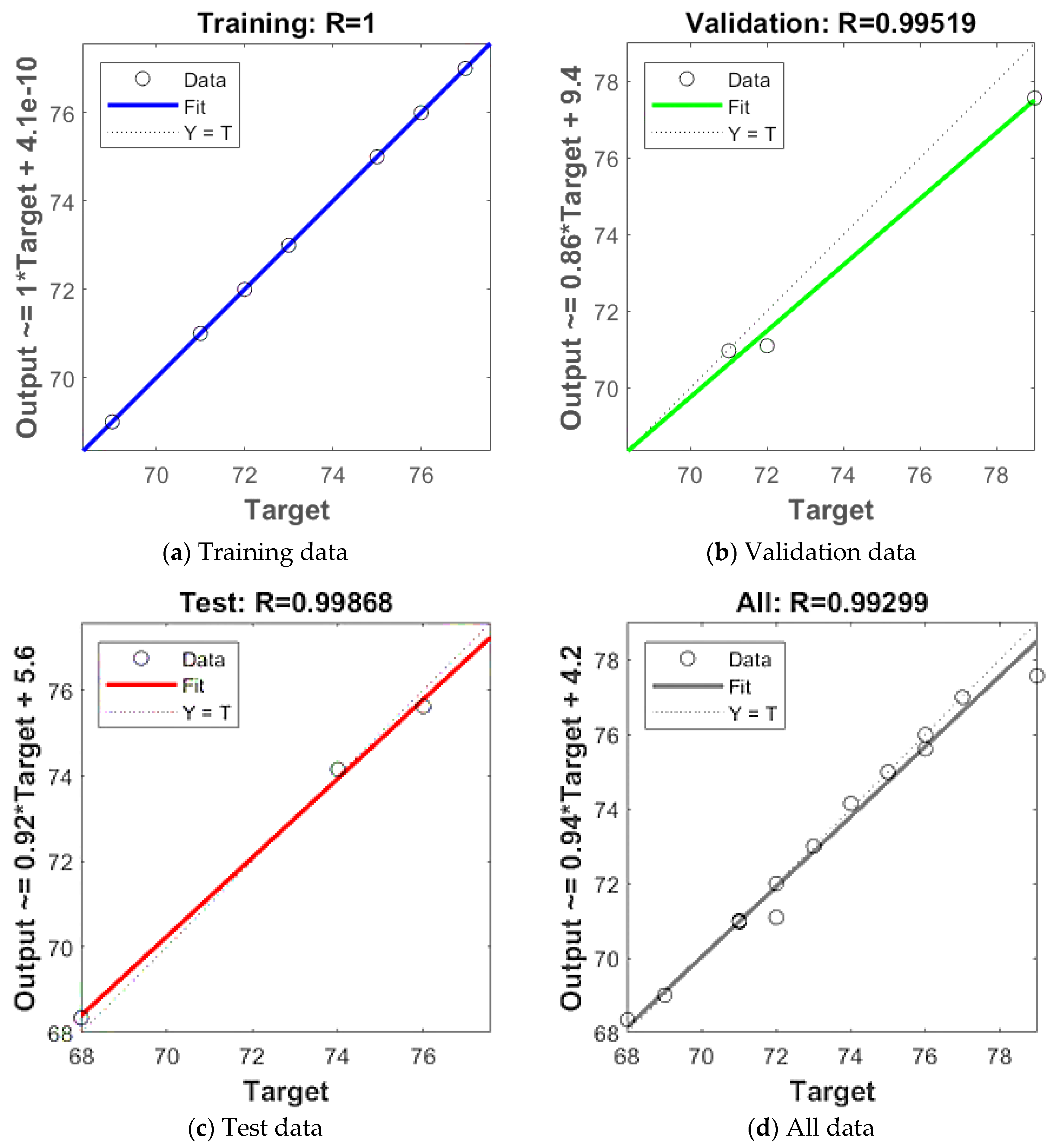
4.1. Validation of Noise Limit Outputs

Seventeen datasets, including all vehicle categories, were calculated and simulated by using the proposed BPNN model in this study. To improve the representativeness of data samples, the dividevec function was used to randomly sort the original data, and randomly extracted 70% of the data as the training data, 15% as the validation data, and the other 15% as the test data. In other words, the training data, validation data and test data were counted as 11, 3, 3, respectively. The predicted results by using the proposed BPNN model are shown in

Table 4. Comparisons on prediction values extracted from the proposed BPNN model and quadratic regression model.

Categories of Vehicle		CNL	BPNN Model			Quadratic Regression Model
			Data Classification	PV	PE	Prediction Model	PV	PE
M1	1	68	Test data	68.34	−0.50%	y = 0.0714x2 − 2.9857x + 85.2	67.80	0.30%
	2	69	Training data	69.00	0.00%	y = 0.1429x2 − 3.2571x + 85.4	69.60	−0.86%
	3	71	Validation data	70.96	0.05%	y = 0.2857x2 − 3.8000x + 85.8	73.20	−3.10%
M2	1	69	Training data	69.00	0.00%	y = 0.2321x2 − 4.4821x + 88.5	68.50	0.73%
	2	71	Training data	71.00	0.00%	y = 0.3750x2 − 5.0250x + 88.9	72.10	−1.55%
	3	72	Training data	72.00	0.00%	y = 0.3750x2 − 5.5679x + 93.3	72.70	−0.97%
	4	72	Validation data	71.09	1.26%	y = 0.2321x2 − 4.9964x + 95.3	71.70	0.42%
M3	1	73	Training data	73.00	0.00%	y = 0.4464x2 − 5.8393x + 93.5	74.50	−2.05%
	2	76	Test data	75.61	0.51%	y = 0.4464x2 − 5.8107x + 95.9	77.10	−1.45%
	3	77	Training data	77.00	0.00%	y = 0.5000x2 − 5.8714x + 95.8	79.20	−2.86%
N1	1	69	Training data	69.00	0.00%	y = 0.1071x2 − 3.4357x + 87.4	68.60	0.58%
	2	71	Training data	71.00	0.00%	y = 0.1071x2 − 2.9786x + 86.8	71.20	−0.28%
N2	1	74	Test data	74.15	−0.21%	y = 0.2321x2 − 4.5393x + 93.7	73.30	0.95%
	2	75	Training data	75.00	0.00%	y = 0.0893x2 − 3.2821x + 92.3	73.70	1.73%
N3	1	76	Training data	76.00	0.00%	y = 0.3750x2 − 5.0821x + 94.1	76.90	−1.18%
	2	77	Validation data	77.00	0.00%	y = 0.5357x2 − 6.3214x + 98.0	79.99	−3.90%
	3	79	Training data	77.57	1.81%	y = 0.6964x2 − 7.0750x + 98.7	83.30	−5.44%

. For comparison, the quadratic regression model was also used, and its predicted results are also given in the same time, in which the least squares method were used to fit the first six historic noise limits to obtain a quadratic regression model, and then the predicted value for the variable set was calculated. In addition, the percentage error (PE) can be determined by

$$PE=\frac{(CNL-PV)}{CNL}\times 100\%$$

(7)

where, $CNL$ is the current noise limit in UNECE regulations, and $PV$ is predicted value by using the proposed BPNN model or the quadratic regression model, respectively.

According to the data, shown in Table 4, the following research findings can be obtained:

(1)

For the training data, the predicted values by using the proposed BPNN model with network learning is almost the same as the values of the current noise limits except for one case for N3 with a percentage error of 1.81%. The quadratic regression model extracted the predicted values with much higher errors from −5.44% to 1.73%. It demonstrated the proposed BPNN model was accurate.

(2)

As for those validation data and test data, since there was no network learning, the predicted values have much larger errors compared with those training data. However, the maximum deviation is still smaller than the results obtained by the quadratic regression model in most cases. Again, the proposed BPNN model provides a better accuracy than the quadratic regression model in the prediction of noise limits during vehicle acceleration.

(3)

The proposed BPNN model can predict noise limits for all learned categories of vehicles, which are only related to historic values of the noise limits of a vehicle, but not depending on its category. Differently, the quadratic regression model is strongly related to both historic values of noise limits of a vehicle and its vehicle category.

(4)

The proposed BPNN model has a migration ability on the prediction of noise limits and can be used to predict the backward trend of noise limits defined in the UNECE regulations. If the inputs of the BPNN model are moved one unit backward, it provides predicted values of noise limits in the next revisions of the UNECE regulations.

Furthermore, a regression analysis of the outputs of the proposed BPNN model was conducted, and the results are shown in Figure 3. The dots in Figure 3 are the abscissa as the vehicle acceleration noise limits as the expected outputs, and the ordinates are the corresponding data points of the predicted limits by using the BPNN model. The dotted line is the ideal curve assuming that the actual output is equal to the expected output; and the solid line is the data point regression analysis and gives the linear regression equation and correlation coefficient.

Table 5. Correlations of the prediction values from the proposed BPNN and those from its regression analysis.

Item	Training Data		Validation Data		Test Data		All Data
	BPNN	Regression	BPNN	Regression	BPNN	Regression	BPNN	Regression
Correlation	1	0.995	0.995	0.999	0.999	0.987	0.993	0.952
Two-tailed test	0.000	0.000	0.013	0.006	0.006	0.013	0.009	0.007

provides the correlations of the results from the proposed BPNN and those from its regression analysis.

It can be found from Table 5 and Figure 3 that the correlation coefficient of each data is very high, and the regression curve of the output point of the neural network is also close to the ideal output curve, indicating that the proposed BPNN model has a strong capability in predicting noise limits emitted by motor vehicles.

4.2. Prediction of Noise Limits for Future Revision of UNECE Regulations

In this section, according to the development trend of noise limits defined in UNECE R51 regulations, the proposed BPNN model is employed to predict the new noise limits of motor vehicles for the future revisions of UNECE regulations. By using its migration ability, shifting one unit of values from the original noise limits backwards, that is, the proposed BPNN model updates the noise limits specified in the second to seventh as inputs to replace those from first to sixth in the regulations, and they are used to predict the noise limits for the next eighth revision of the regulations.

The predicted values of these noise limits of all vehicle categories are shown in

Table 6. Predicted values by using the proposed BPNN model.

Categories of Vehicle		Current Noise Limits with Revision Number 7	Predicted Noise Limits for Next Revision (Revision Number 8)	CR
M1	1	68	69.14	1.68%
	2	69	69.40	0.58%
	3	71	69.83	−1.65%
M2	1	69	69.89	1.28%
	2	71	69.95	−1.48%
	3	72	69.59	−3.34%
	4	72	69.82	−3.03%
M3	1	73	70.45	−3.49%
	2	76	72.23	−4.97%
	3	77	72.26	−6.15%
N1	1	69	69.19	0.27%
	2	71	69.16	−2.59%
N2	1	74	69.57	−5.99%
	2	75	70.73	−5.70%
N3	1	76	70.63	−7.07%
	2	77	73.03	−5.15%
	3	79	73.75	−6.64%

. To better express the trend and law of the future noise limits, a change rate (CR) can be determined by

$$CR=\frac{CN{L}_{n+1}-CN{L}_n}{CN{L}_n}\times 100\%(n=1,2,3,4,5,6,7)$$

(8)

where, $CN{L}_n$ is noise limits with revision number $n$ standing for different versions of UNECE regulations. According to the CR with revision number 7, there are two scenarios, either positive or negative:

(1) The negative rate of change indicates that the vehicle noise limits are becoming stricter, which is conducive to the popularisation and promotion of new automotive technology on vehicle vibration control and noise reduction. It is in line with the development theme of traffic noise control in an urban city, but the cost of noise control would be high.

(2) On the contrary, a positive rate of change indicates that automotive noise limits become looser, which is not conducive to provide better automobile products. In such four cases in M1, M2 and N1 categories, the existing noise limits are suggested being maintained reasonably, and it also suggests the current noise limits are already very strict.

Large fluctuations in the rate of change mainly occur in such a category of vehicles with higher current noise limits than others. The objective of next revision of the regulations on noise limits will focus on reducing the noise limits of these categories of vehicle, such as N2 and N3, sharing technologies to reduce vibrations and noises on all categories of vehicles, and improving the quality of automobile products.

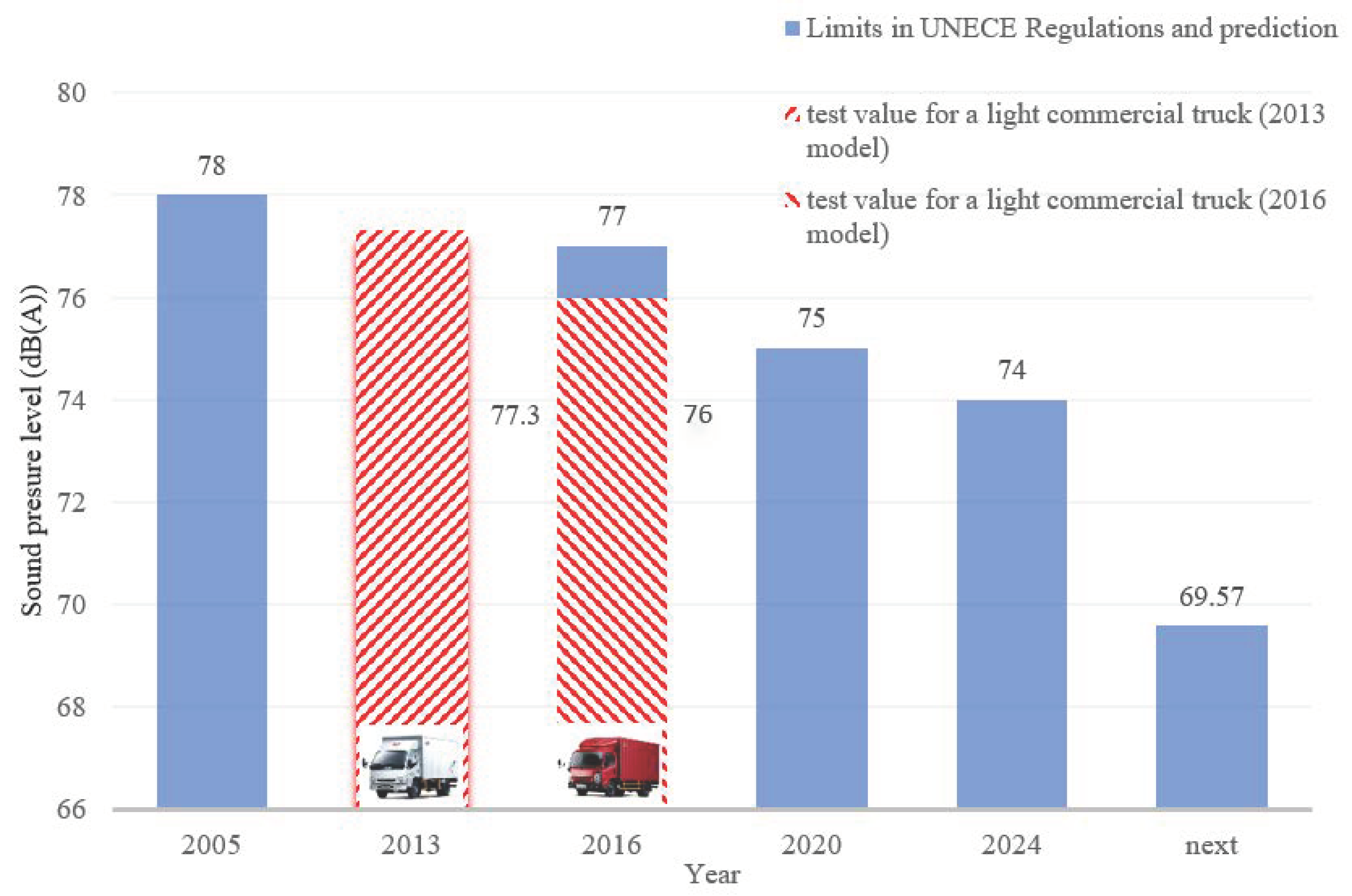
4.3. A Case Study of Noise Control for a Light Commercial Truck

The noise levels of two light commercial trucks made in 2013 and 2016 were measured by Applus+ IDIADA according to the ECE R51 regulations, respectively. There two tested vehicles are the two-generation products from the same motor manufacturer–Jiangling Motors Co., Ltd. (JMC, Nanchang, China). The maximum engine power of the two tested vehicles is 80 kW, and the masses are 4.5 and 4.3 tons, respectively. Therefore, they can be classified to a light commercial truck (vehicle category N2). The sound pressures of the vehicle during accelerating were collected. The sound pressure of the truck made in 2013 (The 2013 model) is 77.3 dB (A), while that of its descendent made in 2016 (The 2016 model) is 76 dB(A) as shown Figure 4. The noise level of the 2013 model is lower than the noise limit specified in UNECE regulations at the time (2005) with a value of 0.7 dB(A), in which the regulations maintained unchanged until 2016. The noise level of the 2016 model is lower than that of specified in the regulations in 2016 with a larger value of 1 dB(A). Apparently, both two tested vehicles meet the requirements of the UNECE regulations. Note that the noise limits in the regulations increase, and become much stricter than before, and the noise level of the Category N2 vehicles during accelerating decreases by 1.3 dB(A). To make sure the fulfilment of the UNECE regulation requirements, the automotive industry strictly follows the regulations on their next-generation product development. The 2020 model could be able to meet the requirements of the current regulations in 2020 and even 2024, if the manufacturer has its product improvements achieved. Unfortunately, the 2020 model was not measured, due to the impacts of COVID-19. However, the next-generation models will face challenges to satisfy the predicted limit of the next revised regulations in future years for the change may be 4.43 dB(A), by using the proposed BPNN model in this research. The predicted value of 69.57 can be used as a reference noise limit for the motor manufacturer to use for their next-generation vehicle design.

5. Concluding Remarks

This study has established a BPNN machine learning model for predicting external noise limits during motor vehicles’ acceleration. The proposed model includes three layers, in which the input layer uses the first six historic data of the vehicle noise limits as inputs, the single hidden layer with 12 neural units id located in the middle, and the output layer is to output the predicted noise limits of motor vehicles.

For validation and verification, the BPNN model was compared with the quadratic regression model. The maximum deviation of the predicted values of the BPNN was found much smaller than those obtained by the quadratic regression model. Those results also demonstrated that the predicted value of the noise limits by using the BPNN model is much close to the expected value of vehicle noises and superior to the quadratic regression model as the percentage errors are much smaller. The BPNN model can also provide a unified function suitable for all learned categories of vehicle and related to the previous noise limits of a car type.

Limits of the external noise limits of all categories of vehicle during accelerating have been predicted by following the trend of noise limits in UNECE R51 regulations. The predicted results show that some categories of vehicles, including N2 and N3, have higher vehicle noise limits defined in the regulations currently and they were predicted to be significantly smaller than the current limits in their next revisions and meanwhile the noise limits of other vehicle categories with low noise limits might be changed slightly.

The proposed BPNN model also has deficiencies, such as the determination of the structure of the neural networks, especially the algorithm of determining the number of hidden layer neurons, in which an optimal value cannot be determined. It would be part of the future work as an extension of current research. For improving the accuracy of the proposed BPNN model for prediction of noise limits of motor vehicles.

References

1. Singh, N.; Davar, S.C. Noise pollution-sources, effects and control. J. Hum. Ecol. 2004, 16, 181. [Google Scholar] [CrossRef]
2. Moore, D. Development of ECE R51. 03 Noise Emission Regulation; SAE Technical Paper 2017-01-1893; SAE International: Warrendale, PA, USA, 2017. [Google Scholar] [CrossRef]
3. Roo, F.D. New EU and UN/ECE Vehicle noise emission limits and associated measurement methods. In Proceedings of the 42nd International Congress and Exposition on Noise Control Engineering-Noise Control for Quality of Life-INTER-NOISE 2013, Innsbruck, Austria, 15–18 September 2013; pp. 6415–6430. [Google Scholar]
4. Sottek, R.; Krebber, W.; Genuit, K. Simulation of vehicle exterior noise. In Proceedings of the Inter-Noise 2001—International Congress and Exhibition on Noise Control Engineering, The Hague, The Netherlands, 28–30 August 2001; pp. 2371–2374. [Google Scholar]
5. McBride Granda, S.M. A Wave Propagation Approach for Prediction of Tire-Pavement Interaction Noise. Ph.D. Thesis, Virginia Tech, Blacksburg, VA, USA, 2019. [Google Scholar]
6. Sarkan, B.; Stopka, O.; Li, C. The issues of measuring the exterior and interior noise of road vehicles. Commun. Sci. Lett. Univ. Zilina 2017, 19, 50. [Google Scholar]
7. Phan, V.L.; Tanaka, H.; Nagatani, T.; Wakamatsu, M.; Yasuki, T. A CFD analysis method for prediction of vehicle exterior wind noise. Sae Int. J. Passeng. Cars Mech. Syst. 2017, 10, 286. [Google Scholar] [CrossRef]
8. Baudet, G.; Dutrion, C.; Lorenzi, R.; Gendre, F.; Geng, S. Calculation Process with Lattice Boltzmann and Finite Element Methods to Choose the Best Exterior Design for Wind Noise. In Proceedings of the Noise and Vibration Conference & Exhibition, Grand Rapids, MI, USA, 10−13 June 2017. [Google Scholar]
9. Nygren, J.; Boij, S.; Rumpler, R.; O’Reilly, C.J. A study of the interaction between vehicle exterior noise emissions and vehicle energy demands for different drive cycles. In Proceedings of the 23rd International Congress on Acoustics, ICA, Aachen, Germany, 9–13 September 2019. [Google Scholar]
10. Kerber, S. The importance of vehicle exterior noise levels in urban traffic for pedestrian—Vehicle interaction. Atz Worldw. 2006, 108, 19. [Google Scholar] [CrossRef]
11. Tousignant, T.; Eisele, G.; Govindswamy, K.; Steffens, C.; Tomazic, D. Optimization of Electric Vehicle Exterior Noise for Pedestrian Safety and Sound Quality. In Proceedings of the INTER-NOISE and NOISE-CON Congress and Conference Proceedings, Grand Rapids, MI, USA, 12–14 June 2017; Institute of Noise Control Engineering: Reston, VA, USA; pp. 245–252. [Google Scholar]
12. Qi, J.; Du, J.; Siniscalchi, S.M.; Ma, X.; Lee, C.H. Analyzing Upper Bounds on Mean Absolute Errors for Deep Neural Network Based Vector-to-Vector Regression. IEEE Trans. Signal Process. 2020, 68, 3411–3422. [Google Scholar] [CrossRef]
13. Nourani, V.; Gökçekuş, H.; Umar, I.K.; Najafi, H. An emotional artificial neural network for prediction of vehicular traffic noise. Sci. Total Environ. 2020, 707, 136134. [Google Scholar] [CrossRef]
14. Jiménez-Romero, F.J.; Guijo-Rubio, D.; Lara-Raya, F.R.; Ruiz-González, A.; Hervás-Martínez, C. Validation of artificial neural networks to model the acoustic behaviour of induction motors. Appl. Acoust. 2020, 166, 107332. [Google Scholar] [CrossRef]
15. Lu, H.; Wang, T. An Automobile Noise Prediction Model Based on Extension Data Mining Algorithm. Rev. D’intelligence Artif. 2019, 33, 341. [Google Scholar] [CrossRef]
16. Çelebi, K.; Uludamar, E.; Tosun, E.; Yıldızhan, Ş.; Aydın, K.; Özcanlı, M. Experimental and artificial neural network approach of noise and vibration characteristic of an unmodified diesel engine fuelled with conventional diesel, and biodiesel blends with natural gas addition. Fuel 2017, 197, 159. [Google Scholar] [CrossRef]
17. Huang, B.; Pan, Z.; Liu, Z.; Hou, G.; Yang, H. Acoustic amenity analysis for high-rise building along urban expressway: Modeling traffic noise vertical propagation using neural networks. Transp. Res. Part D Transp. Environ. 2017, 53, 63. [Google Scholar] [CrossRef]
18. Steinbach, L.; Altinsoy, M.E. Prediction of annoyance evaluations of electric vehicle noise by using artificial neural networks. Appl. Acoust. 2019, 145, 149. [Google Scholar] [CrossRef]
19. Werbos, P.J. Beyond Regression: New Tools for Prediction and Analysis in the Behavioral Sciences. Ph.D. Thesis, Harvard University, Cambridge, MA, USA, 1974. [Google Scholar]
20. Bhat, N.; McAvoy, T.J. Use of neural nets for dynamic modeling and control of chemical process systems. Comput. Chem. Eng. 1990, 14, 573. [Google Scholar] [CrossRef]
21. Rumelhart, D.E.; Hinton, G.E.; Williams, R.J. Learning representations by back-propagating errors. Nature 1986, 323, 533. [Google Scholar] [CrossRef]
22. Khashei, M.; Bijari, M. An artificial neural network (p, d, q) model for timeseries forecasting. Expert Syst. Appl. 2010, 37, 479. [Google Scholar] [CrossRef]
23. Han, J.; Moraga, C. The influence of the sigmoid function parameters on the speed of backpropagation learning. In International Workshop on Artificial Neural Networks; Springer: Berlin, Germany, 1995; p. 195. [Google Scholar]
24. Kreinovich, V.; Sirisaengtaksin, O. 3-layer neural networks are universal approximations for functions and for control strategies. Neural Parallel Sci. Comp. 1993, 1, 325. [Google Scholar]
25. Beheshti, M.; Berrached, A.; de Korvin, A.; Hu, C.; Sirisaengtaksin, O. On interval weighted three-layer neural networks. In Proceedings of the 31st Annual Simulation Symposium, Boston, MA, USA, 5–9 April 1998; IEEE: Piscataway Township, NJ, USA, 1998; p. 188. [Google Scholar]
26. Gavin, H.P. The Levenberg-Marquardt Algorithm for Nonlinear Least Squares Curve-Fitting Problems. Department of Civil and Environmental Engineering, Duke University. Available online: http://people.duke.edu/~hpgavin/ce281/lm.pdf (accessed on 1 October 2020).
27. Mirri, S.; Delnevo, G.; Roccetti, M. Is a COVID-19 Second Wave Possible in Emilia-Romagna (Italy)? Forecasting a Future Outbreak with Particulate Pollution and Machine Learning. Computation 2020, 8, 74. [Google Scholar] [CrossRef]
28. Joachims, T. Learning to Classify Text Using Support Vector Machines; Springer Science & Business Media: Berlin, Germany, 2002. [Google Scholar]
29. Cortes, C.; Vapnik, V. Support-vector networks. Mach. Learn. 1995, 20, 273. [Google Scholar] [CrossRef]
30. Williams, C.K.; Rasmussen, C.E. Gaussian Processes for Machine Learning; MIT Press: Cambridge, MA, USA, 2006. [Google Scholar]
31. Rasmussen, C.E. Gaussian processes in machine learning. In Summer School on Machine Learning; Springer: Berlin, Germany, 2003; p. 63. [Google Scholar]
32. Dietterich, T.G. Ensemble methods in machine learning. In International Workshop on Multiple Classifier Systems; Springer: Berlin, Germany, 2000; p. 1. [Google Scholar]
33. Sagi, O.; Rokach, L. Ensemble learning: A survey. Wiley Interdiscip. Rev. Data Min. Knowl. Discov. 2018, 8, e1249. [Google Scholar] [CrossRef]
34. Steinberg, D.; Colla, P. CART: Classification and regression trees. Top Ten Algorithms Data Min. 2009, 9, 179. [Google Scholar]
35. Rodriguez-Galiano, V.; Sanchez-Castillo, M.; Chica-Olmo, M.; Chica-Rivas, M. Machine learning predictive models for mineral prospectivity: An evaluation of neural networks, random forest, regression trees and support vector machines. Ore Geol. Rev. 2015, 71, 804. [Google Scholar] [CrossRef]
Figure 1. Schematic diagram of neural network architecture.
Applsci 10 08092 g001
Figure 2. The proposed architecture of the back-propagation neural network (BPNN) model for noise limits during vehicle acceleration (6–12–1).
Applsci 10 08092 g002
Figure 3. Relationships between prediction values from the BPNN model and current noise limits.
Applsci 10 08092 g003
Figure 4. Comparisons on limits and test values for light commercial trucks (Category N2).
Applsci 10 08092 g004