An Effective Multi-Label Feature Selection Model Towards Eliminating Noisy Features

Abstract

Feature selection has devoted a consistently great amount of effort to dimension reduction for various machine learning tasks. Existing feature selection models focus on selecting the most discriminative features for learning targets. However, this strategy is weak in handling two kinds of features, that is, the irrelevant and redundant ones, which are collectively referred to as noisy features. These features may hamper the construction of optimal low-dimensional subspaces and compromise the learning performance of downstream tasks. In this study, we propose a novel multi-label feature selection approach by embedding label correlations (dubbed ELC) to address these issues. Particularly, we extract label correlations for reliable label space structures and employ them to steer feature selection. In this way, label and feature spaces can be expected to be consistent and noisy features can be effectively eliminated. An extensive experimental evaluation on public benchmarks validated the superiority of ELC.

1. Introduction

For pattern recognition, feature selection is important for its effectiveness in reducing dimensionality. Feature selection methods are divided into supervised, semi-supervised, and unsupervised ones, according to whether the instances are labeled, partially labeled, or not [1,2,3,4]. For supervised cases, class labels are employed for measuring features’ discriminative abilities. Many popular and efficient feature selection methods belong to this group [5,6,7,8,9,10]. Supervised methods are further categorized into three well-known models: filter, wrapper, and embedded [11]. In recent years, some hybrid methods have emerged that combine filter and wrapper processes for enhancing performance and reducing computational cost [12,13].

In another categorization view, existing feature selection approaches can also be grouped to single-label and multi-label ones, whose difference lies in the size of labels that each instance is related with [14]. In single-label FS, instances and labels hold many-to-one connections and the target separability is emphasized in this learning task. With the great potential and success of multi-label learning in many machine learning fields, such as text categorization [15], content annotation [16], and protein location prediction [17], multi-label feature selection has received considerable attention in recent years. We approach the supervised multi-label feature selection in this study.

In multi-label learning, label correlations are the key to combining the complicated relationships among instances, which are typically annotated with multiple labels [18,19]. The mainstream multi-label feature selection strategy is to extract label correlations (via statistical or information-based measurements) and employ them to help find the most remarkable features. A critical issue is, however, this strategy would be trapped by two kinds of features, that is, irrelevant and redundant ones. Irrelevant features represent those lowly discriminative ones. Features of this kind are loosely correlated with learning targets and even may provide misleading information. Compared with irrelevant features, redundant features seem more deceptive. They may exhibit excellent (or comparably superior) performances and mix with remarkable features. Nevertheless, redundant features also lowly contribute to enhancing the discriminative ability of the constructed low-dimensional subspace, because the learning information they provide is redundant with the already distilled information. In general, we regard both irrelevant and redundant features as noisy ones, which may confuse selection processes and compromise the learning performance of downstream tasks.

In this paper, we present an effective multi-label feature selection model by embedding label correlations to eliminate noisy features, named ELC. Our major strategy is to keep feature-label space consistent and explore reliable label structures to drive feature selection. Concretely, we qualitatively assess label correlations in the label space and embed them in feature selection. In this way, the label structure information can be maximally preserved in the constructed low-dimensional subspace, and eventually the consistency between feature and label spaces can be achieved. Furthermore, we devise an efficient framework base on the sparse multi-task learning to optimize ELC, which can help ELC find globally optimal solutions and efficiently converge.

The major contributions of this paper are as follows:

• We present a novel multi-label feature selection model to address the issue of noisy features. This model qualitatively measures label correlations and employs feature-label space consistency to steer feature selection.
• We devised a compact framework to optimize the proposed model. This framework resorts to the multi-task learning strategy and promises globally optimal solutions and efficient convergence.
• Comprehensive experiments on openly available benchmarks were conducted to validate the performance of the proposed model in feature selection and noise elimination.

The remaining parts of this paper are arranged as follows: related works are reviewed in Section 2; the proposed model ELC and its optimization framework are respectively introduced in Section 3 and Section 4; the experimental comparisons of ELC with several popular feature selection approaches are presented in Section 5; finally, conclusions are drawn in Section 6.

2. Related Work

Feature selection approaches are commonly specified to a certain recognition scenario, i.e., single-label learning or multi-label learning, because of the different concerns of the two recognition tasks. The issue of noisy feature elimination is firstly raised in single-label feature selection, focusing on removing irrelevant features and picking out discriminative ones. For example, the popular single-label feature selection family by preserving instance similarity [20] directly highly scores the most discriminative features under various statistical metrics, such as the Laplacian score [7,21], the Fisher score [6], the Hilbert–Schmidt independence criterion [22], and the trace ratio [23], just to name a few. In addition to the above similarity preservation approaches, some traditional distance or instance difference based ones can also be deemed as simply pursuing “target-specific features,” such as ReliefF [10], SPEC [24,25], and SPFS [20]. This denotation arises from the fact that target-specific features are picked based only on whether they are strongly correlated with the learning targets. In other words, those features that have excellent discriminative abilities for targets will prevail. The aforementioned approaches have generally achieved excellent performance in eliminating irrelevant features, while may experience difficulties in improving learning performance due to their scarce attention on removing redundant features.

Recently, some remarkable neural networks-based and fuzzy logic-based feature selection works have been presented, which have received extensive attention due to their excellent feature selection performances [26,27,28]. For example, Verikas and Bacauskiene [26] proposed a feedforward neural network-based approach to find the salient features and remove those yielding the least accurate classifications. Arefnezhad et al. [27] highly scored the features most related to the drowsiness level via an adaptive neuro-fuzzy inference system, which was devised by combining filter and wrapper feature selection approaches. Cateni et al. [28] selected the mostly relevant features for better binary classification by combining several filter approaches through a fuzzy inference system. Generally speaking, the above studies serve as excellent examples of picking out target-specific features, while still leaving aside the underlying negative effects of noisy features.

A salient but redundant feature provides little valuable learning information if selected. Although this issue is ignored by a majority of feature selection approaches, it gains attention from some information-based ones. Among them, the family based on mutual information is regarded as the mainstream redundancy removing approach. The classical mutual information [9] and its variants (e.g., conditional mutual information) [5,29] can effectively position the redundant features and remove them via a greedy search. Nevertheless, an inevitable problem is that the performances of these approaches heavily depend on their probability estimation accuracy. This problem is more complicated in high-dimensional space.

In terms of multi-label feature selection approaches, they can be roughly categorized into two families. The first family directly divides the multi-label learning into multiple subproblems and utilizes single-label feature evaluation metrics to tackle them [4]. For instance, ReliefF is tailed for multi-label learning by dividing its estimations of nearest misses and hits to eight subproblems [30]. In addition, some single-label feature evaluation strategies are also reformulated to the multi-label ones by enforcing on each subgroup, such as class separability and linear discriminant analysis [31,32]. A major drawback of the above subproblem division strategy is that it ignores label correlations, which encode the underlying label structures for recognition and play critical roles in multi-label learning.

On the other hand, the second family of multi-label feature selection can better fix this issue since it incorporates label correlations into model construction. A common strategy of this family is to evaluate instance-label pairs via specific label ranking metrics and select the features by minimizing loss functions [33,34,35,36]. While real-world label relations could be beyond pairwise situations, some high-order correlation approaches have been proposed to model complicated label structures. A feasible solution is to build a common space shared among various labels [16,33,37], which typically suffers from high costs and complex computation. It is noteworthy that in contrast to single-label feature selection approaches, the multi-label ones rarely have the issue of noisy feature elimination. A few approaches specific to ruling out irrelevant features are based on sparse regularization [38]. These approaches neglect the negative effects of redundant features and are not competent in completely removing noisy features.

To comprehensively address the above issues, we will introduce a novel multi-label feature selection model in Section 3, which can effectively filter both kinds of noisy features (including irrelevant and redundant ones) and select the remarkable ones. The proposed model adopts a statistical metric to measure target-related feature redundancy and dispense with any probability estimation. Furthermore, this model extracts label correlations and keeps feature-label space consistency to guide feature selection, which facilitates irrelevant feature exclusion and remarkable feature domination.

3. The Methodology: ELC

3.1. Model Description

In this paper, we use ${\{{\mathbf{x}}_i,{\mathbf{y}}_i\}}_{i=1}^n$ to denote the data set, where $\mathbf{X}=[{\mathbf{x}}_1;\dots ;{\mathbf{x}}_n]\in {\mathbb{R}}^{n\times d}$ represents the instance matrix and instances are characterized by d features in the feature set $\mathbf{F}=\{{\mathbf{f}}_1,\dots ,{\mathbf{f}}_d\}$. $\mathbf{Y}=[{\mathbf{y}}_1,\dots ,{\mathbf{y}}_l]\in {\{0,1\}}^{n\times l}$ denotes the target label matrix, where $y_{ij}=1$ represents a positive label and $y_{ij}=0$ corresponds to a negative one.

Then, we formulate the multi-label feature selection by embedding label correlation (ELC) as follows:

$$\begin{array}{cc}\hfill & \underset{\mathbf{W}}{min}\frac{1}{2}{∥{\widehat{\mathbf{Y}}}^T\widehat{\mathbf{Y}}-\mathbf{S}∥}_F^2,s.t.\widehat{\mathbf{Y}}=\frac{1}{n}{\left(\mathbf{X}\mathbf{W}\right)}^T\mathbf{Y},\mathbf{W}\in {\{0,1\}}^{d\times l},{∥\mathbf{W}∥}_{2,0}=k,\hfill \end{array}$$

(1)

where $\mathbf{S}\in {\mathbb{R}}^{l\times l}$ represents the label correlation matrix calculated over the initial label matrix, and k is the number of selected features. $\mathbf{W}\in {\mathbb{R}}^{d\times l}$ is the feature selection matrix, where $w_{ij}$ indicates the importance (also known as weight) of the i-th feature to the j-th label.

Equation (1) is actually the feature evaluation function of ELC, which is essentially a Frobenius-norm quadratic model. The matrix $\mathbf{S}$ represents the label correlations extracted from the label space, and its each element describes a relation between two target labels. These correlations can be easily obtained by some quantitative measurements, including RBF kernel function, Pearson correlation coefficient, etc. ${\widehat{\mathbf{Y}}}^T\widehat{\mathbf{Y}}$ represents the label correlations extracted from the reduced feature space. ${\widehat{\mathbf{Y}}}^T\widehat{\mathbf{Y}}$ is differentiated from $\mathbf{S}$ on account of the disturbance of noisy features. As described in Section 1, noisy features may distort the structure of the feature space and provide negative learning information. Considering this, ELC evaluates features based on their abilities of preserving label correlations in the feature space, that is, keeping feature-label space consistency. The features that can minimize the discrepancy between ${\widehat{\mathbf{Y}}}^T\widehat{\mathbf{Y}}$ and $\mathbf{S}$ will be highly scored by ELC. In this way, ELC can be expected to construct an optimal feature subspace with eliminating different kinds of noisy features.

Under the constraint of the ${\ell }_{2,0}$-norm in Equation (1), only k row in $\mathbf{W}$ is nonzero. This corresponds to the k selected features for l target labels, where 1 represents selected and 0 represents none. Note that k is most likely to be unequal to l. That is, more than one feature may be selected responsible for discriminating the same label, or only one feature is discriminative for more than one label. In the former case, multiple features are unified to recognize one target, while one feature deals with multiple recognition sub-tasks in the latter case.

3.2. Property Analysis

The feature subset $\widehat{\mathbf{F}}=\left\{{\widehat{\mathbf{f}}}_1,{\widehat{\mathbf{f}}}_2,\dots ,{\widehat{\mathbf{f}}}_k\right\}$ that is selected by ELC can be considered as maximally maintaining feature-label space consistency. $\widehat{\mathbf{F}}$ is expected to be constituted by the remarkable features and exclude the noisy ones. In this subsection, we will further analyze the properties of ELC and reveal its underlying characteristics.

Suppose that each feature in $\mathbf{F}$ has been standardized to have mean zero and unit length. Then, the following things hold for Equation (1):

$${∥{\widehat{\mathbf{Y}}}^T\widehat{\mathbf{Y}}-\mathbf{S}∥}_F^2={∥\frac{1}{n^2}\left({\mathbf{Y}}^T\left(\mathbf{X}\mathbf{W}\right){\left(\mathbf{X}\mathbf{W}\right)}^T\mathbf{Y}\right)-\mathbf{S}∥}_F^2.$$

This is the objective of ELC. For more clearly illustrating its properties, let $\widehat{\mathcal{S}}=n^2\mathbf{S}$ and $\mathcal{H}={\mathbf{Y}}^T\left(\mathbf{X}\mathbf{W}\right){\left(\mathbf{X}\mathbf{W}\right)}^T\mathbf{Y}$. Then,

$$\begin{array}{cc}\hfill & {∥{\widehat{\mathbf{Y}}}^T\widehat{\mathbf{Y}}-\mathbf{S}∥}_F^2=\frac{1}{n^2}\left(tr\left({\mathcal{H}}^T\mathcal{H}\right)+tr\left({\widehat{\mathcal{S}}}^T\widehat{\mathcal{S}}\right)-2tr\left({\widehat{\mathcal{S}}}^T\mathcal{H}\right)\right).\hfill \end{array}$$

Three terms are involved in this equation. Clearly, $tr\left({\widehat{\mathcal{S}}}^T\widehat{\mathcal{S}}\right)$ represents the label correlation information extracted from the label space and is constant in the selection process. Thus, it is easy to conclude that $\underset{\mathbf{W}}{min}{∥{\widehat{\mathbf{Y}}}^T\widehat{\mathbf{Y}}-\mathbf{S}∥}_F^2$ is equivalent to $\underset{\mathbf{W}}{min}tr\left({\mathcal{H}}^T\mathcal{H}\right)$ and $\underset{\mathbf{W}}{max}tr\left({\widehat{\mathcal{S}}}^T\mathcal{H}\right)$. Then, two properties of ELC are given as follows:

Property 1.

Label correlation information can be maximally embedded in feature selection by ELC.

Proof. 

$tr\left({\widehat{\mathcal{S}}}^T\mathcal{H}\right)=tr\left({\left(\mathbf{XW}\right)}^T\mathbf{Y}\widehat{\mathcal{S}}{\mathbf{Y}}^T\left(\mathbf{XW}\right)\right)$$={\sum }_{i=1}^k{\widehat{\mathbf{f}}}_i^T\left(\mathbf{Y}\widehat{\mathcal{S}}{\mathbf{Y}}^T\right){\widehat{\mathbf{f}}}_i={\sum }_{i=1}^k{\widehat{\mathbf{f}}}_i^T\left({\displaystyle \sum _{c1=1}^l}{\displaystyle \sum _{c2=1}^l}{\mathbf{y}}_{c1}{s}_{c1,c2}{\mathbf{y}}_{c2}^T\right){\widehat{\mathbf{f}}}_i$, where $s_{c1,c2}$ is the correlation degree of the labels ${\mathbf{y}}_{c1}$ and ${\mathbf{y}}_{c2}$, and $\mathbf{XW}$ indicates the selected features. Then, the following things holds: $\underset{\mathbf{W}}{min}{∥{\widehat{\mathbf{Y}}}^T\widehat{\mathbf{Y}}-\mathbf{S}∥}_F^2\propto \underset{\mathbf{W}}{max}{\sum }_{i=1}^k{\widehat{\mathbf{f}}}_i^T\left({\sum }_{c1=1}^l{\sum }_{c2=1}^l{\mathbf{y}}_{c1}{s}_{c1,c2}{\mathbf{y}}_{c2}^T\right){\widehat{\mathbf{f}}}_i$. ${\sum }_{c1=1}^l{\sum }_{c2=1}^l{\mathbf{y}}_{c1}{s}_{c1,c2}{\mathbf{y}}_{c2}^T$ can be regarded as the correlation information of pairwise labels. Therefore, ELC can maximally embed label correlations in its feature selection process. □

Label correlation information is important for multi-label learning. For example, the images about seas may share some common labels for recognition, such as ship, fish, and seagull, and their close correlations may help us distinguish the image category and find their shared features. The existing multi-label learning methods are categorized on the basis of the label correlation orders they consider [39]. Their correlation modeling capabilities directly affect their discriminative performance. As demonstrated in Property 1, ELC can measure the pairwise label correlations. Furthermore, it can also preserve this correlation information in its constructed feature subspace, which is crucial for ELC to eliminate noisy features. In other words, the features that can maximally preserve label correlation information are preferred by ELC. This strategy facilitates ELC building a low-dimensional feature space that is consistent with the label space and also suitable for multi-label learning.

In addition to the above property with respect to maximally embedding label correlations, another important property of ELC is illustrated as follows:

Property 2.

Feature redundancy can be minimized by ELC.

Proof. 

$tr\left({\mathcal{H}}^T\mathcal{H}\right)={\sum }_{i,j=1}^k{\left(\left({\widehat{\mathbf{f}}}_i^T\mathbf{Y}\right){\left({\widehat{\mathbf{f}}}_j^T\mathbf{Y}\right)}^T\right)}^2$$={\sum }_{i,j=1}^k{\sum }_{c=1}^l{\left(\langle {\widehat{\mathbf{f}}}_i,{\mathbf{y}}_c\rangle \langle {\widehat{\mathbf{f}}}_j,{\mathbf{y}}_c\rangle \right)}^2$

$={\sum }_{i,j=1}^k{\sum }_{c=1}^l{n}^4{\sigma }_{{\mathbf{y}}_c}^4{\rho }_{{\widehat{\mathbf{f}}}_i,{\mathbf{y}}_c}^2{\rho }_{{\widehat{\mathbf{f}}}_j,{\mathbf{y}}_c}^2,$ where ${\sigma }_{{\mathbf{y}}_c}$ is the standard deviation of the label ${\mathbf{y}}_c$, and ${\rho }_{{\widehat{\mathbf{f}}}_i,{\mathbf{y}}_c}$ and ${\rho }_{{\widehat{\mathbf{f}}}_j,{\mathbf{y}}_c}$ are the Pearson correlation coefficients of ${\mathbf{y}}_c$ with the features ${\widehat{\mathbf{f}}}_i$ and ${\widehat{\mathbf{f}}}_j$, respectively. Then, we have $\underset{\mathbf{W}}{min}{∥{\widehat{\mathbf{Y}}}^T\widehat{\mathbf{Y}}-\mathbf{S}∥}_F^2\propto \underset{\mathbf{W}}{min}{\sum }_{i,j=1}^k{\sum }_{c=1}^l{n}^4{\sigma }_{{\mathbf{y}}_c}^4{\rho }_{{\widehat{\mathbf{f}}}_i,{\mathbf{y}}_c}^2{\rho }_{{\widehat{\mathbf{f}}}_j,{\mathbf{y}}_c}^2.$

Clearly, n and ${\sigma }_{{\mathbf{y}}_c}$ are constant in the feature selection process. ${\sum }_{c=1}^l{\rho }_{{\widehat{\mathbf{f}}}_i,{\mathbf{y}}_c}{\rho }_{{\widehat{\mathbf{f}}}_j,{\mathbf{y}}_c}$ can be regarded as the shared label dependency of the features ${\widehat{\mathbf{f}}}_i$ and ${\widehat{\mathbf{f}}}_j$, that is, the feature redundancy for recognizing the target ${\mathbf{y}}_c$. Therefore, ELC can minimize feature redundancy in its feature selection process. □

Note that the term ${\sum }_{c=1}^l{\rho }_{{\widehat{\mathbf{f}}}_i,{\mathbf{y}}_c}{\rho }_{{\widehat{\mathbf{f}}}_j,{\mathbf{y}}_c}$ in Property 2 is obtained by introducing the label correlation information. This is a completely novel estimation for the label-specific feature redundancy. The most majority of existing feature selection approaches (including the single-label and multi-label ones) adopt a univariate measurement criterion and merely the top-k features have opportunities to prevail. This strategy largely increases the redundant recognition information shared between features. For example, if we select the genes that are all discriminative for the diabetes type 1, we probably cannot give an accurate diagnosis since these features may be less aware of other types of diabetes. This is why we have to reduce recognition redundancy and enrich recognition information. Some approaches are able to reduce feature redundancy, while their focus is not the label-specific redundancy. For example, ${\sum }_{i,j=1}^k{\rho }_{{\widehat{\mathbf{f}}}_i,{\widehat{\mathbf{f}}}_j}$ is actually reduced in SPFS [20]. This term includes an additional information irrelevant to recognition, and correspondingly, it is inappropriate. In contrast, ELC removes label-specific feature redundancy and is more suitable for multi-label learning with eliminating noisy features.

As discussed above, ELC processes two properties, i.e., maximally preserving label correlation information and minimizing label-specific feature redundancy. These characteristics account for the superior ability of ELC in eliminating noisy features and picking out remarkable ones.

4. Multi-Task Optimization for ELC

Equation (1) describes an integer programming problem, which is NP-hard and complicated to solve. Moreover, the ${\ell }_{2,0}$-norm constraint in Equation (1) is non-smooth, which leads to a slow convergence rate. In this section, we devise an efficient framework to address this problem by using the sparse multi-task learning technology in the proximal alternating direction method (PADM) framework [40].

Suppose the spectral decomposition of the correlation matrix $\mathbf{S}$ can be denoted as

$$\mathbf{S}=\mathsf{\Phi }\mathsf{\Sigma }{\mathsf{\Phi }}^T=\mathsf{\Phi }diag({\sigma }_1,\dots ,{\sigma }_l){\mathsf{\Phi }}^T,{\sigma }_1\ge \dots \ge {\sigma }_l,$$

where $\mathsf{\Phi }$ and $\mathsf{\Sigma }$ are respectively the eigenvector and eigenvalue matrices of $\mathbf{S}$. Then, Equation (1) can be reformulated as

$$\begin{array}{cc}\hfill & \underset{\mathbf{W},\mathbf{p}}{min}\frac{1}{2}{∥{\mathbf{Y}}^T\mathbf{X}diag\left(\mathbf{p}\right)\mathbf{W}-{\mathsf{\Gamma }}^{*}∥}_F^2,s.t.\mathbf{W}\in {\mathbb{R}}^{d\times l},{∥\mathbf{W}∥}_{2,1}\le t,\mathbf{p}\in {\{0,1\}}^d,{\mathbf{p}}^T\mathbf{1}=k,\hfill \end{array}$$

(2)

where ${\mathsf{\Gamma }}^{*}=n\mathsf{\Phi }{\mathsf{\Sigma }}^{1/2}$, t is a hyperparameter to constrain ${∥\mathbf{W}∥}_{2,1}$ to a convex solution, $\mathbf{p}$ is a feature indicator vector that reflects whether the corresponding features are selected or not (1 for selected and 0 for otherwise), and $\mathbf{1}$ is the vector with all ones.

On the basis of Equation (2), ELC is actually reformulated as a multivariate regression problem, which enables the multi-task learning technology [41]. This technology aims to learn a common set of features to tackle multiple relevant tasks and excels at various sparse learning formulations, including the optimization problem in Equation (1). Based on the multi-task learning technology, we then obtain the equivalent form of ELC as follows:

$$\begin{array}{cc}\hfill & \underset{\mathbf{W},\mathbf{p}}{min}\frac{1}{2}{∥\widehat{\mathbf{A}}diag\left(\mathbf{p}\right)\mathbf{W}-{\mathsf{\Gamma }}^{*}∥}_F^2+\lambda {∥\mathbf{W}∥}_{2,1},s.t.\mathbf{p}\in {\{0,1\}}^d,{\mathbf{p}}^T\mathbf{1}=k,\hfill \end{array}$$

(3)

where $\widehat{\mathbf{A}}={\mathbf{Y}}^T\mathbf{X}$, and $\lambda >0$ is the regularization parameter. Clearly, we can apply the augmented Lagrangian method to solve this problem. Then, Equation (3) is further reformulated as

$$\begin{array}{cc}\hfill & \underset{\mathbf{U},\mathbf{W},\mathbf{p}}{min}\frac{1}{2}{∥\widehat{\mathbf{A}}diag\left(\mathbf{p}\right)\mathbf{W}-{\mathsf{\Gamma }}^{*}∥}_F^2+\lambda {∥\mathbf{U}∥}_{2,1},s.t.\mathbf{U}=\mathbf{W},\mathbf{p}\in {\{0,1\}}^d,{\mathbf{p}}^T\mathbf{1}=k.\hfill \end{array}$$

(4)

The Lagrangian function can be defined as

$$\begin{array}{cc}\hfill & \mathcal{L}(\mathbf{U},\mathbf{W},\mathbf{p},\mathbf{V})=\frac{1}{2}{∥\widehat{\mathbf{A}}diag\left(\mathbf{p}\right)\mathbf{W}-{\mathsf{\Gamma }}^{*}∥}_F^2+\frac{\beta }{2}{∥\mathbf{W}-\mathbf{U}∥}^2+\lambda {∥\mathbf{U}∥}_{2,1}-tr\left({\mathbf{V}}^T(\mathbf{W}-\mathbf{U})\right),\hfill \end{array}$$

(5)

where $\mathbf{V}={\left({\mathbf{v}}_1^T,\dots ,{\mathbf{v}}_d^T\right)}^T\in {\mathbb{R}}^{d\times l}$ is the Lagrangian multiplier, and $\beta >0$ is the penalty parameter.

Equation (5) involves four variables, that is, the auxiliary variable $\mathbf{U}$, the feature weight matrix $\mathbf{W}$, the feature indicator vector $\mathbf{p}$, and the Lagrangian multiplier $\mathbf{V}$. Clearly, simultaneously optimizing four variables is impractical. Accordingly, $\mathbf{V}$ is temporarily fixed for simplification in the following analysis. Then, minimizing $\mathcal{L}(\mathbf{U},\mathbf{W},\mathbf{p},\mathbf{V})$ is equivalent to the following two subproblems; i.e.,

• $\underset{\mathbf{U}}{min}{\mathcal{L}}_1\left(\mathbf{U}\right)=\underset{\mathbf{U}}{min}\frac{\beta }{2}{∥\mathbf{W}-\mathbf{U}∥}^2+\lambda {∥\mathbf{U}∥}_{2,1}+tr\left({\mathbf{V}}^T\mathbf{U}\right);$
• $\underset{\mathbf{W},\mathbf{p}}{min}{\mathcal{L}}_2(\mathbf{W},\mathbf{p})=\underset{\mathbf{W},\mathbf{p}}{min}\frac{1}{\beta }{∥\widehat{\mathbf{A}}diag\left(\mathbf{p}\right)\mathbf{W}-{\mathsf{\Gamma }}^{*}∥}_F^2+{∥\mathbf{W}-\mathbf{U}∥}^2$$-\frac{2}{\beta }tr\left({\mathbf{V}}^T\mathbf{W}\right).$

As to ${\mathcal{L}}_1\left(\mathbf{U}\right)$, the following holds:

$${\mathcal{L}}_1\left(\mathbf{U}\right)={\sum }_{i=1}^d\left(\frac{\beta }{2}{∥{\mathbf{w}}^i-{\mathbf{u}}^i∥}^2+\lambda ∥{\mathbf{u}}^i∥+tr\left({\mathbf{v}}_i^T{\mathbf{u}}^i\right)\right),$$

(6)

where ${\mathbf{w}}^i$ and ${\mathbf{u}}^i$ are the i-th row vectors of $\mathbf{W}$ and $\mathbf{U}$, respectively. Then, we reformulate $\underset{\mathbf{U}}{min}{\mathcal{L}}_1\left(\mathbf{U}\right)$ to its close form [41] as

$$\underset{{\mathbf{u}}^i}{min}{\sum }_{i=1}^d\left(\frac{\beta }{2}{∥{\mathbf{w}}^i-{\mathbf{u}}^i+\frac{1}{\beta }{\mathbf{v}}_i∥}^2+\lambda ∥{\mathbf{u}}^i∥\right).$$

(7)

Conducting gradient descent on Equation (7) yields the following optimal solution as

$${\mathbf{u}}^i=max\left\{∥{\mathbf{w}}^i+\frac{1}{\beta }{\mathbf{v}}_i∥-\frac{\lambda }{\beta },0\right\}\frac{{\mathbf{w}}^i+\frac{1}{\beta }{\mathbf{v}}_i}{∥{\mathbf{w}}^i+\frac{1}{\beta }{\mathbf{v}}_i∥}.$$

(8)

Then, the optimal $\mathbf{U}$ in iteration $[t+1]$ can be denoted as

$${\mathbf{U}}^{[t+1]}=max\left\{∥{\mathbf{W}}^{\left[t\right]}+\frac{1}{\beta }{\mathbf{V}}^{\left[t\right]}∥-\frac{\lambda }{\beta },0\right\}\frac{{\mathbf{W}}^{\left[t\right]}+\frac{1}{\beta }{\mathbf{V}}^{\left[t\right]}}{∥{\mathbf{W}}^{\left[t\right]}+\frac{1}{\beta }{\mathbf{V}}^{\left[t\right]}∥}.$$

(9)

In terms of $\underset{\mathbf{W},\mathbf{p}}{min}{\mathcal{L}}_2(\mathbf{W},\mathbf{p})$, we let $\mathcal{P}=\left\{\mathbf{p}\right|\mathbf{p}\in {\{0,1\}}^d,{\mathbf{p}}^T\mathbf{1}=k\}$. The dual problem of $\underset{\mathbf{W},\mathbf{p}}{min}{\mathcal{L}}_2(\mathbf{W},\mathbf{p})$ is

$$\underset{\mathbf{p}\in \mathcal{P}}{min}\underset{\mathbf{W}}{max}{\mathcal{L}}_2(\mathbf{W},\mathbf{p}).$$

(10)

Since simultaneously solving the both variables $\mathbf{p}$ and $\mathbf{W}$ is still tough, we first fix $\mathbf{p}$ to optimize $\mathbf{W}$. Then, the solution of $\mathbf{W}$ can be obtained as

$$\left(diag\left(\mathbf{p}\right){\widehat{\mathbf{A}}}^T\widehat{\mathbf{A}}diag\left(\mathbf{p}\right)-\beta \mathbf{I}\right)\mathbf{W}=diag\left(\mathbf{p}\right){\widehat{\mathbf{A}}}^T{\mathsf{\Gamma }}^{*}+\beta \mathbf{U}+\mathbf{V},$$

(11)

where $\mathbf{I}$ is the identity matrix. The structure of ${\widehat{\mathbf{A}}}^T\widehat{\mathbf{A}}$ is commonly not circulant, and therefore the computation of Equation (11) is involved [42]. Considering this, an approximate term is added to ${\mathcal{L}}_2(\mathbf{W},\mathbf{p})$ as follows:

$$\begin{array}{cc}\hfill & {\tilde{\mathcal{L}}}_2(\mathbf{W},\mathbf{p})=\frac{1}{\beta \tau }∥\mathbf{W}-{\mathbf{W}}^{\left[t\right]}+\tau {\mathsf{\Omega }}^{\left[t\right]}∥-\frac{2}{\beta }tr\left({\mathbf{V}}^T\mathbf{W}\right)+{∥\mathbf{W}-\mathbf{U}∥}^2,\hfill \\ \hfill & {\mathsf{\Omega }}^{\left[t\right]}=diag\left({\mathbf{p}}^{\left[t\right]}\right){\widehat{\mathbf{A}}}^T\left(\widehat{\mathbf{A}}diag\left({\mathbf{p}}^{\left[t\right]}\right){\mathbf{W}}^{\left[t\right]}-{\mathsf{\Gamma }}^{*}\right),\hfill \end{array}$$

(12)

where $\tau >0$, and ${\mathbf{W}}^{\left[t\right]}$ is the optimal value of $\mathbf{W}$ in iteration $\left[t\right]$. Then, the solution of ${\mathbf{W}}^{[t+1]}$ is

$${\mathbf{W}}^{[t+1]}=\left(\frac{\tau }{\beta \tau +1}\right)\left(\beta {\mathbf{U}}^{[t+1]}+{\mathbf{V}}^{\left[t\right]}+\frac{1}{\tau }({\mathbf{W}}^{\left[t\right]}-\tau {\mathsf{\Omega }}^{\left[t\right]})\right).$$

(13)

The detailed inference can be found in the Appendix A.

Similarly, we can easily obtain the optimal $\mathbf{p}$ by fixing $\mathbf{W}$. Equation (10) is then equivalent to the following minimization problem in this case as follows:

$$\underset{\mathbf{p}\in \mathcal{P}}{min}{∥\widehat{\mathbf{A}}diag\left(\mathbf{p}\right)\mathbf{W}-{\mathsf{\Gamma }}^{*}∥}_F^2=\underset{\mathbf{p}\in \mathcal{P}}{min}{∥{\mathbf{Y}}^T{\sum }_{i=1}^d{p}_i{\mathbf{f}}_i{\mathbf{w}}^i-{\mathsf{\Gamma }}^{*}∥}_F^2.$$

(14)

Apparently, the top-k features that minimize ${∥{\mathbf{Y}}^T{\mathbf{f}}_i{\mathbf{w}}^i-{\mathsf{\Gamma }}^{*}∥}_F^2$ can be regarded as the remarkable ones. Their corresponding values in $\mathbf{p}$ are assigned as 1.

Note that the Lagrangian multiplier $\mathbf{V}$ is fixed through the above analysis, mainly for simplifying the solution process. We further tackle this problem in the popular PADM framework as illustrated in Algorithm 1. In this framework, $\mathbf{V}$ can be updated as

$${\mathbf{V}}^{[t+1]}={\mathbf{V}}^{\left[t\right]}-\beta \left({\mathbf{W}}^{[t+1]}-{\mathbf{U}}^{[t+1]}\right).$$

(15)

Algorithm 1 ELC

input:  $\mathbf{F}=\left\{{\mathbf{f}}_1,\dots ,{\mathbf{f}}_d\right\},\mathbf{Y},\mathbf{S},k,\beta ,\tau ,\lambda$ output:  ${\mathbf{p}}^{\left[t\right]}$ 1: begin 2: $t=0,{\mathbf{W}}^{\left[0\right]}={\mathbf{0}}_{d\times l},{\mathbf{U}}^{\left[0\right]}={\mathbf{0}}_{d\times l},{\mathbf{V}}^{\left[0\right]}=\frac{1}{d}{\mathbf{1}}_{d\times l}$; 3: find top-k features ${\widehat{\mathbf{f}}}_1^{\left[0\right]},\dots ,{\widehat{\mathbf{f}}}_k^{\left[0\right]}$ that minimize Equation (1), and set $p_i^{\left[0\right]}=\left\{\begin{array}{c}1,{\mathbf{f}}_i\in \left\{{\widehat{\mathbf{f}}}_1^{\left[0\right]},\dots ,{\widehat{\mathbf{f}}}_k^{\left[0\right]}\right\}\hfill \\ 0,otherwise\hfill \end{array}\right.$; 4: while “not converged” do 5:       optimize ${\mathbf{U}}^{[t+1]}$ according to Equation (9); 6:       optimize ${\mathbf{W}}^{[t+1]}$ according to Equation (13); 7:       find top-k features ${\widehat{\mathbf{f}}}_1^{[t+1]},\dots ,{\widehat{\mathbf{f}}}_k^{[t+1]}$ which minimize Equation (14), and set $p_i^{[t+1]}=\left\{\begin{array}{c}1,{\mathbf{f}}_i\in \left\{{\widehat{\mathbf{f}}}_1^{[t+1]},\dots ,{\widehat{\mathbf{f}}}_k^{[t+1]}\right\}\hfill \\ 0,otherwise\hfill \end{array}\right.$; 8:       update ${\mathbf{V}}^{[t+1]}$ according to Equation (15); 9:       $t=t+1$; 10: end while; 11: return${\mathbf{p}}^{\left[t\right]}$; 12: end;

ELC in Algorithm 1 is implemented in the regression framework PADM, which is a fast alternating approach for the well-known alternating direction method (ADM) framework. PADM is effective and efficient in solving the minimization problem of the augmented Lagrangian function, and is able to converge to a certain solution $\left\{{\mathbf{W}}^{*},{\mathbf{U}}^{*}\right\}$ from any starting point $\left\{{\mathbf{W}}^{\left[0\right]},{\mathbf{U}}^{\left[0\right]}\right\}$ for any $\beta >0$ [40].

In terms of the complexity of ELC, it only takes $O(klogd)$ time to find k remarkable features from the d candidates. Thus, the time consumption for line 3 is $O(nd{l}^2+klogd)$. The cost of the while loop in Algorithm 1 mainly lies in lines 6 and 7, which is $O(d^2{l}^2+nd{l}^2+klogd)$. As this iteration process is repeated for t times, its total cost is $O\left(t(d^2{l}^2+nd{l}^2+klogd)\right)$. Suppose $t\gg 1$. Then, the total complexity of ELC is approximately equal to $O\left(t(d^2{l}^2+nd{l}^2+klogd)\right)$, where $d,n,l,k,t$ are the numbers of features, instances, labels, selected features, and iterations for convergence, respectively.

5. Experimental Evaluation

Fourteen groups of multi-label data sets fetched from the Mulan library (http://mulan.sourceforge.net/datasets-mlc.html) are taken as the benchmarks in this section, which are shown in

Table 1. Benchmarks for multi-label feature selection.

Data Set	♯Features	♯Instances	♯Labels	Domain
emotions	72	539	6	music
yeast	103	2417	14	biology
birds	260	645	19	audio
enron	1001	1702	53	text
genbase	1186	662	27	biology
business	21,924	11,214	30	text
arts	23146	7484	26	text
education	27,534	12,030	33	text
reaction	30,324	12,828	22	text
health	30,605	9205	32	text
computers	34,096	12,444	33	text
science	37,187	6428	40	text
reference	39,679	8027	33	text
society	49,060	14,512	22	text

. We compare ELC (the source code is available at https://github.com/wangjuncs/ELC) with the following state-of-the-art multi-label feature selection methods:

• MIFS (multi-label informed feature selection) [33]: a label correlation-based multi-label feature selection approach, which maps label information into a low-dimensional subspace and captures the correlations among multiple labels;
• CMFS (correlated and multi-label feature selection) [35]: a feature selection approach based on non-negative matrix factorization, which exploits the label correlation information in features, labels, and instances to select the relevant features and remove the noisy ones;
• LLSF (learning label-specific features) [36]: a unified multi-label learning framework for both feature selection and classification, which models high-order label correlations to select label-specific features.

More detailed experimental configurations can be found in the Appendix B.

5.1. Example 1: Classification Performance

The average classification performance of each feature selection approach is recorded in

Table 2. Average multi-label classification performance (mean $\pm$ std.): the best results and those not significantly worse than it are highlighted in bold (pairwise t-test at 5% significance level).

(a) Precision (the higher the better).
Approaches	Data Sets							AVG.
	Emotions	Yeast	Birds	Enron	Genbase	Business	Arts
MIFS	0.6667$\pm$0.04	0.7520$\pm$0.02	0.3938$\pm$0.02	0.6139$\pm$0.03	0.7361$\pm$0.15	0.8812$\pm$0.00	0.5108$\pm$0.01	0.6506
CMFS	0.7221$\pm$0.02	0.7464$\pm$0.01	0.4116$\pm$0.03	0.6206$\pm$0.01	0.7342$\pm$0.15	0.892$\pm$0.00	0.5611$\pm$0.00	0.6697
LLSF	0.7016$\pm$0.02	0.7532$\pm$0.01	0.4231$\pm$0.07	0.6197$\pm$0.04	0.7352$\pm$0.15	0.8924$\pm$0.00	0.5615$\pm$0.01	0.6695
ELC	0.7306$\pm$0.02	0.7564$\pm$0.01	0.4671$\pm$0.08	0.6347$\pm$0.01	0.9868$\pm$0.00	0.8931$\pm$0.00	0.5646$\pm$0.00	0.7190
	Education	Reaction	Health	Computers	Science	Reference	Society
MIFS	0.5129$\pm$0.01	0.5836$\pm$0.01	0.7391$\pm$0.02	0.6629$\pm$0.01	0.4592$\pm$0.02	0.6267$\pm$0.01	0.5899$\pm$0.01	0.5963
CMFS	0.6164$\pm$0.01	0.5883$\pm$0.01	0.7437$\pm$0.01	0.6931$\pm$0.00	0.5477$\pm$0.01	0.6718$\pm$0.01	0.6463$\pm$0.01	0.6439
LLSF	0.6163$\pm$0.01	0.5880$\pm$0.01	0.7435$\pm$0.01	0.6932$\pm$0.00	0.5478$\pm$0.01	0.6720$\pm$0.00	0.6460$\pm$0.01	0.6438
ELC	0.6213$\pm$0.00	0.5952$\pm$0.00	0.7469$\pm$0.01	0.6962$\pm$0.00	0.5565$\pm$0.00	0.6742$\pm$0.00	0.6500$\pm$0.00	0.6486
(b) AUC (the higher the better).
Approaches	Data Sets							AVG.
	Emotions	Yeast	Birds	Enron	Genbase	Business	Arts
MIFS	0.6601$\pm$0.53	0.6554$\pm$0.03	0.6497$\pm$0.02	0.5968$\pm$0.03	0.7886$\pm$0.10	0.6371$\pm$0.01	0.6100$\pm$0.01	0.6568
CMFS	0.7307$\pm$0.03	0.647$3\pm$0.03	0.6403$\pm$0.04	0.6194$\pm$0.01	0.7883$\pm$0.10	0.6821$\pm$0.01	0.6606$\pm$0.01	0.6812
LLSF	0.7069$\pm$0.02	0.6601$\pm$0.02	0.6793$\pm$0.05	0.6092$\pm$0.03	0.7887$\pm$0.10	0.6824$\pm$0.01	0.6608$\pm$0.01	0.6839
ELC	0.7513$\pm$0.02	0.6706$\pm$0.02	0.7018$\pm$0.06	0.6385$\pm$0.01	0.9663$\pm$0.00	0.6834$\pm$0.00	0.6659$\pm$0.00	0.7254
	Education	Reaction	Health	Computers	Science	Reference	Society
MIFS	0.5830$\pm$0.02	0.7065$\pm$0.01	0.6994$\pm$0.01	0.6364$\pm$0.01	0.6109$\pm$0.02	0.6246$\pm$0.01	0.5964$\pm$0.01	0.6423
CMFS	0.6753$\pm$0.00	0.7111$\pm$0.01	0.7014$\pm$0.01	0.6864$\pm$0.01	0.6732$\pm$0.01	0.6674$\pm$0.01	0.6430$\pm$0.01	0.6867
LLSF	0.6761$\pm$0.01	0.7114$\pm$0.01	0.7032$\pm$0.01	0.6859$\pm$0.01	0.6723$\pm$0.01	0.6672$\pm$0.01	0.6427$\pm$0.01	0.6867
ELC	0.6779$\pm$0.00	0.7188$\pm$0.01	0.7053$\pm$0.01	0.6905$\pm$0.00	0.6789$\pm$0.00	0.6681$\pm$0.01	0.6465$\pm$0.00	0.6911
(c) Hamming loss (the lower the better).
Approaches	Data Sets							AVG.
	Emotions	Yeast	Birds	Enron	Genbase	Business	Arts
MIFS	0.2865$\pm$0.02	0.2006$\pm$0.01	0.0538$\pm$0.00	0.0544$\pm$0.00	0.0303$\pm$0.02	0.0270$\pm$0.00	0.0610$\pm$0.00	0.1019
CMFS	0.2600$\pm$0.01	0.2031$\pm$0.01	0.0535$\pm$0.00	0.0527$\pm$0.00	0.0303$\pm$0.02	0.0253$\pm$0.00	0.0568$\pm$0.00	0.0974
LLSF	0.2697$\pm$0.01	0.1999$\pm$0.01	0.0532$\pm$0.00	0.0539$\pm$0.00	0.0303$\pm$0.02	0.0253$\pm$0.00	0.0568$\pm$0.00	0.0984
ELC	0.2517$\pm$0.02	0.1982$\pm$0.01	0.0518$\pm$0.00	0.0523$\pm$0.00	0.0049$\pm$0.00	0.0251$\pm$0.00	0.0567$\pm$0.00	0.0915
	Education	Reaction	Health	Computers	Science	Reference	Society
MIFS	0.0430$\pm$0.00	0.0539$\pm$0.00	0.0373$\pm$0.00	0.0379$\pm$0.00	0.0353$\pm$0.00	0.0317$\pm$0.00	0.0557$\pm$0.00	0.0399
CMFS	0.0371$\pm$0.00	0.0536$\pm$0.00	0.0368$\pm$0.00	0.0350$\pm$0.00	0.0322$\pm$0.00	0.0280$\pm$0.00	0.0511$\pm$0.00	0.0394
LLSF	0.0371$\pm$0.00	0.0536$\pm$0.00	0.0369$\pm$0.00	0.0349$\pm$0.00	0.0322$\pm$0.00	0.0280$\pm$0.00	0.0512$\pm$0.00	0.0394
ELC	0.0368$\pm$0.00	0.0531$\pm$0.00	0.0366$\pm$0.00	0.0348$\pm$0.00	0.0319$\pm$0.00	0.0278$\pm$0.00	0.0508$\pm$0.00	0.0391
(d) Ranking loss (the lower the better).
Approaches	Data Sets							AVG.
	Emotions	Yeast	Birds	Enron	Genbase	Business	Arts
MIFS	0.3154$\pm$0.05	0.1767$\pm$0.01	0.2988$\pm$0.01	0.0986$\pm$0.01	0.0586$\pm$0.03	0.0377$\pm$0.00	0.1510$\pm$0.05	0.1624
CMFS	0.2404$\pm$0.02	0.1810$\pm$0.01	0.2887$\pm$0.02	0.0959$\pm$0.00	0.0594$\pm$0.03	0.0336$\pm$0.00	0.1341$\pm$0.00	0.1476
LLSF	0.2711$\pm$0.02	0.1756$\pm$0.01	0.2777$\pm$0.05	0.0962$\pm$0.01	0.0591$\pm$0.03	0.0335$\pm$0.00	0.1341$\pm$0.00	0.1496
ELC	0.2379$\pm$0.02	0.1733$\pm$0.01	0.2568$\pm$0.05	0.0924$\pm$0.00	0.0065$\pm$0.00	0.0334$\pm$0.00	0.1332$\pm$0.00	0.1334
	Education	Reaction	Health	Computers	Science	Reference	Society
MIFS	0.0988$\pm$0.00	0.1459$\pm$0.01	0.0498$\pm$0.00	0.0820$\pm$0.00	0.1351$\pm$0.01	0.0849$\pm$0.00	0.1372$\pm$0.00	0.0994
CMFS	0.0768$\pm$0.00	0.1438$\pm$0.01	0.0492$\pm$0.00	0.0735$\pm$0.00	0.1112$\pm$0.00	0.0734$\pm$0.00	0.1175$\pm$0.00	0.0897
LLSF	0.0768$\pm$0.00	0.1438$\pm$0.01	0.0492$\pm$0.00	0.0736$\pm$0.00	0.1111$\pm$0.00	0.0736$\pm$0.00	0.1176$\pm$0.00	0.0898
ELC	0.0759$\pm$0.00	0.1405$\pm$0.00	0.0486$\pm$0.00	0.0728$\pm$0.00	0.1085$\pm$0.00	0.0731$\pm$0.00	0.1161$\pm$0.00	0.0883
(e) One error (the lower the better).
Approaches	Data Sets							AVG.
	Emotions	Yeast	Birds	Enron	Genbase	Business	Arts
MIFS	0.4451$\pm$0.05	0.2403$\pm$0.01	0.7226$\pm$0.03	0.3230$\pm$0.03	0.3698$\pm$0.21	0.1187$\pm$0.00	0.6215$\pm$0.01	0.4059
CMFS	0.3871$\pm$0.02	0.2445$\pm$0.01	0.6968$\pm$0.04	0.3093$\pm$0.02	0.3719$\pm$0.21	0.1061$\pm$0.00	0.5518$\pm$0.01	0.3811
LLSF	0.3986$\pm$0.03	0.2387$\pm$0.01	0.6879$\pm$0.08	0.3158$\pm$0.05	0.3707$\pm$0.21	0.1058$\pm$0.00	0.5509$\pm$0.01	0.3812
ELC	0.3664$\pm$0.03	0.2361$\pm$0.01	0.6192$\pm$0.11	0.2988$\pm$0.01	0.0123$\pm$0.00	0.1050$\pm$0.00	0.5464$\pm$0.00	0.3120
	Education	Reaction	Health	Computers	Science	Reference	Society
MIFS	0.6452$\pm$0.02	0.5292$\pm$0.02	0.3335$\pm$0.03	0.4041$\pm$0.01	0.6761$\pm$0.02	0.4743$\pm$0.01	0.4684$\pm$0.01	0.5104
CMFS	0.4989$\pm$0.01	0.5234$\pm$0.02	0.3266$\pm$0.02	0.3738$\pm$0.01	0.5605$\pm$0.02	0.4208$\pm$0.01	0.3933$\pm$0.01	0.4537
LLSF	0.4993$\pm$0.01	0.5237$\pm$0.02	0.3267$\pm$0.02	0.3735$\pm$0.00	0.5605$\pm$0.02	0.4202$\pm$0.01	0.3937$\pm$0.01	0.4536
ELC	0.4923$\pm$0.00	0.5147$\pm$0.01	0.3223$\pm$0.02	0.3699$\pm$0.00	0.5490$\pm$0.01	0.4172$\pm$0.00	0.3885$\pm$0.00	0.4771

and the pairwise t-tests at 5% significance level were conducted to validate the statistical significance. In addition to the traditional precision and AUC metrics, hamming loss penalizes incorrect the recognitions of instances to each target label, ranking loss penalizes the misordered labels in pairs, and one-error penalizes the instances whose top-ranked predicted labels are not in the ground-truth label set. Five metrics evaluated the multi-label classification performance from different aspects.

A single metric is insufficient to illustrate the general classification performance on a dataset. For example, the overall performance of ML-KNN classifier [43] on birds is worse than that on enron under the precision metric, while it shows a better performance on birds than on enron under the AUC metric. Therefore, we extensively used five metrics to compare the performances of the compared approaches. As shown in Table 2, ELC outperforms MIFS, CMFS, and LLSF under various metrics. This superiority is attributed to two reasons. That is, ELC can effectively eliminate noisy features from the candidate feature subsets and maximally embed label correlation information into its selection process. The first term rules out the selection disturbance in the feature space, and the second term promises the proper guiding information extracted from the label space. By seamlessly fusing these two terms, ELC is able to find discriminative features for the downstream learning tasks. This point will be further validated in Section 5.2 and Section 5.3.

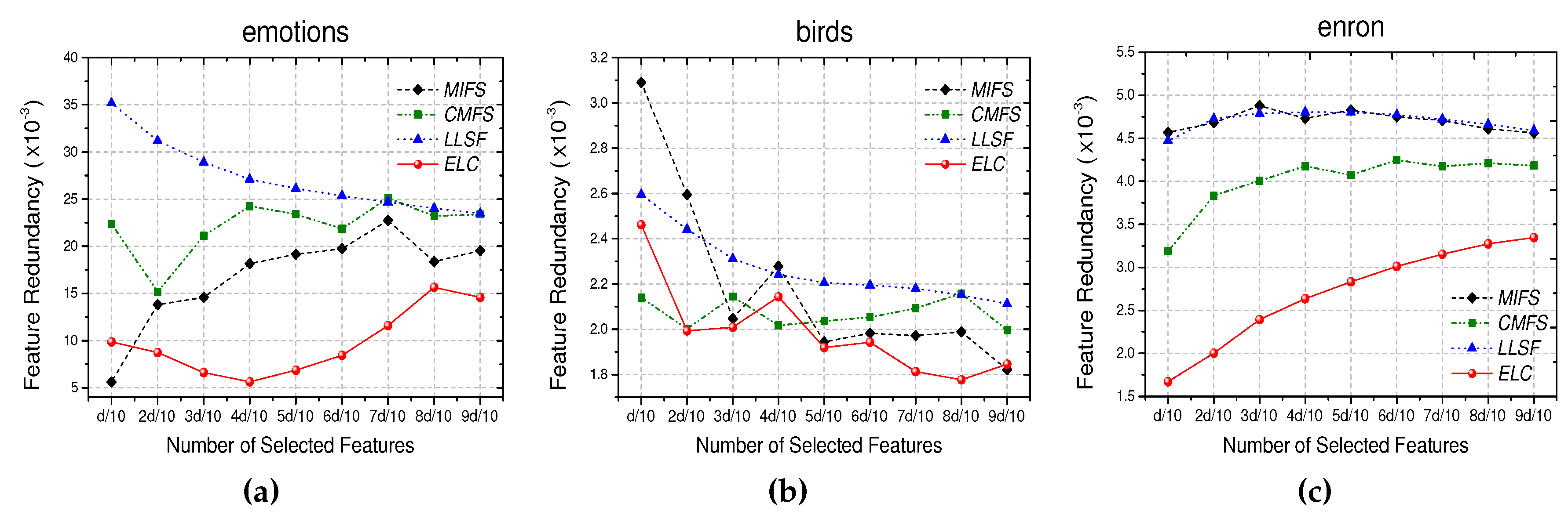
5.2. Example 2: Eliminating Noisy Features

In this section, we evaluate the performances of the compared approaches in eliminating noisy features. We take emotions, birds, and enron as the benchmarks, and measure the residual feature redundancy in the selected feature subset $\widehat{\mathbf{F}}$ as follows:

$$R\left(\widehat{\mathbf{F}}\right)=\frac{1}{k^{\prime }(k^{\prime }-1)l}\sum _{{\widehat{\mathbf{f}}}_i,{\widehat{\mathbf{f}}}_j\in \widehat{\mathbf{F}}}\sum _{c=1}^l{\rho }_{{\widehat{\mathbf{f}}}_i,{\mathbf{y}}_c}^2{\rho }_{{\widehat{\mathbf{f}}}_j,{\mathbf{y}}_c}^2,$$

(16)

where ${\rho }_{{\widehat{\mathbf{f}}}_i,{\mathbf{y}}_c}$ and ${\rho }_{{\widehat{\mathbf{f}}}_j,{\mathbf{y}}_c}$ are the Pearson correlation coefficients of the features ${\widehat{\mathbf{f}}}_i$ and ${\widehat{\mathbf{f}}}_j$ with the target label ${\mathbf{y}}_l$, and $k^{\prime }$ and l are the numbers of the selected features and labels, respectively. When $R\left(\widehat{\mathbf{F}}\right)$ reaches its maximum value, the maximal redundant information exists in $\widehat{\mathbf{F}}$, which interprets as the inferior ability of the selection approach in removing noisy features.

The feature redundancy of $k^{\prime }$ selected features for each approach is demonstrated in Figure 1, where $k^{\prime }\in \{d/10,2d/10,\dots ,9d/10\}$ and d is the total number of original features. It illustrates that ELC is superior in reducing feature redundancy. In other words, ELC can effectively remove redundant features in its multi-label feature selection process. This is one of the crucial factors leading to the excellent discriminative ability of ELC. It should be pointed out that in contrast to the case of single-label feature selection, eliminating noisy features has not received sufficient attention from existing multi-label feature selection approaches. While the issue of noisy features is an obstacle of yielding high selection performance not only for the single-label learning but also for the multi-label cases, we devised ELC to comprehensively tackle this problem. Moreover, the reduced feature redundancy in the majority of redundancy elimination-based approaches is not directly relevant to the target labels. In contrast, ELC quantitatively reduces target-relevant redundancy without any prior probability knowledge, which is conducive to its superiority in multi-label feature selection.

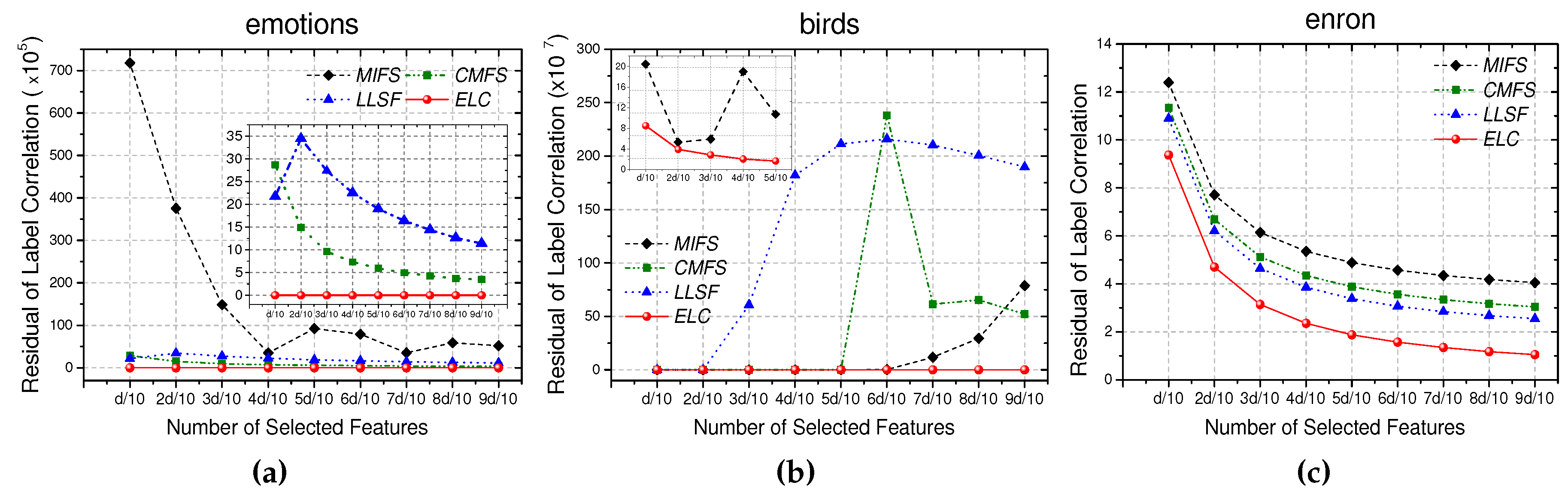
5.3. Example 3: Embedding Label Correlations

Label correlation information is important for multi-label learning. In the following experiments, we estimate the preserved label correlation information of the selected feature subset $\widehat{\mathbf{F}}$ as follows:

$$C\left(\widehat{\mathbf{F}}\right)=\frac{1}{k^{\prime }(k^{\prime }-1)}{∥\frac{1}{n^2}{\mathbf{Y}}^T{\mathbf{X}}_{\widehat{\mathbf{F}}}{\mathbf{X}}_{\widehat{\mathbf{F}}}^T\mathbf{Y}-\mathbf{S}∥}_F^2,$$

(17)

where ${\mathbf{X}}_{\widehat{\mathbf{F}}}$ denotes the instances characterized by $\widehat{\mathbf{F}}$ and $\mathbf{S}$ is the label correlation matrix of the original data. Intuitively, Equation (17) measures the residue scale of label correlation information in the original and reduced feature spaces. A lower value indicates more information preserved. In other words, more label correlation information can be embedded in the feature selection process in this situation.

Similarly to the configuration in Section 5.2, we take emotions, birds, and enron as the benchmarks and record $C\left(\widehat{\mathbf{F}}\right)$ of the $k^{\prime }$ features selected by each approach, where $k^{\prime }\in \{d/10,2d/10,\dots ,9d/10\}$. As shown in Figure 2, ELC is better at preserving the class correlation information than the other multi-label feature selection approaches. Actually, the majority of the existing multi-label feature selection approaches take the label correlation information into consideration to some extent. In contrast to these approaches, ELC quantitatively measures this correlation information and maximally embeds it into the feature selection process. This characteristic, which has already been proved in Property 2, can be further revealed by the experimental results in this section.

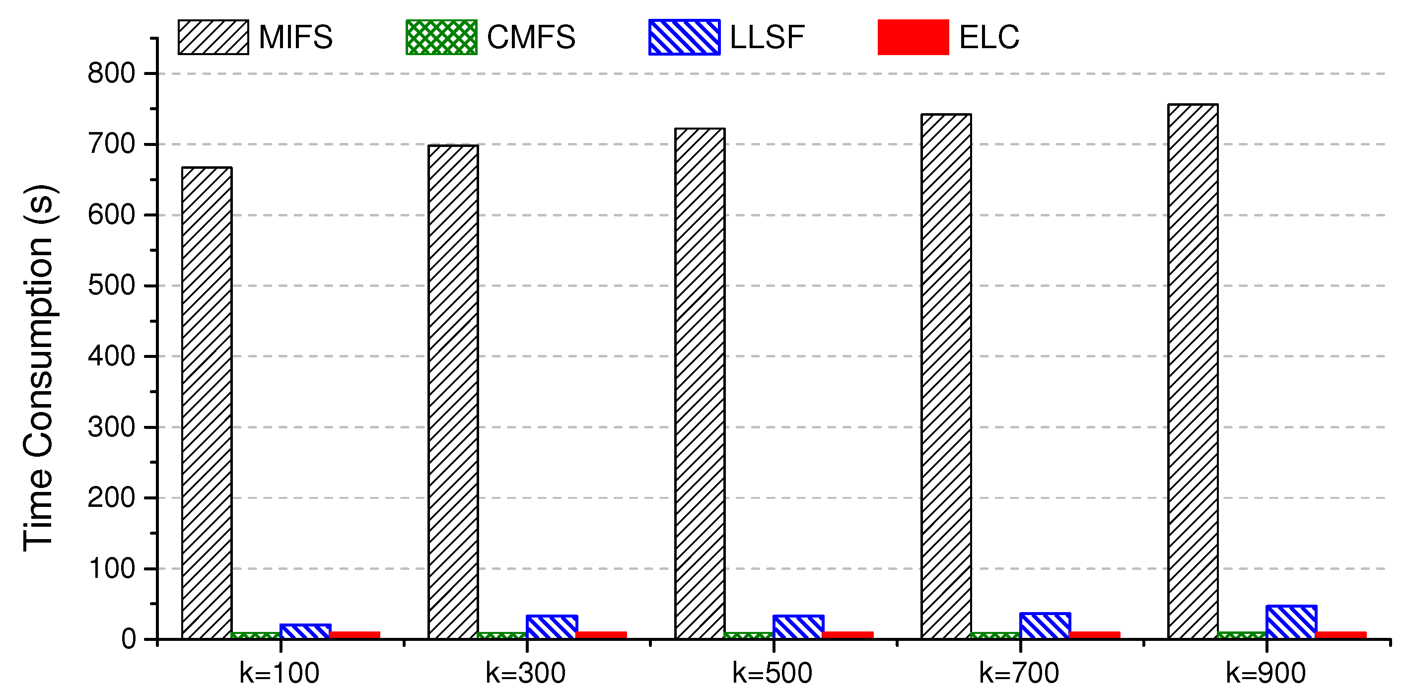
5.4. Example 4: Time Consumption

In this section, we compare the approaches in terms of their feature selection efficiency. The time consumption here merely records the feature selection time, excluding the classification cost. All of the tests were implemented in Matlab on an Intel Core i7-4790 CPU (@3.6GHz) with 32GB memory (Intel Corp., Santa Clara, CA, USA). We respectively selected $k^{\prime }$ ($k^{\prime }\in \{100,300,500,700,900\}$) features on the enron dataset and recorded the time consumption of each compared approach. As illustrated in Figure 3, ELC and CMFS are comparably efficient to converge, while MIFS is most time-consuming, which may be mainly attributed to its involved label clustering process.

6. Conclusions

A novel multi-label feature selection method called ELC is proposed in this paper. ELC embeds label correlation information in reduced feature subspace to eliminate noisy features. In this way, irrelevant and redundant features can be expected to be removed and a discriminative feature subset is constructed for the downstream learning tasks. These advantages help ELC yield good feature selection performance on a wide broad of multi-label data sets under various evaluation metrics.

In terms of optimizing ELC, we can feed it to some gradient descent frameworks to efficiently yield its optimal values, such as Adam with a self-adaptive learning rate [44]. Another interesting and possible exploration would be the consideration of noisy labels, which would induce negative effects on estimating label correlations. According to our pilot study, noisy labels may distort the label space and provide inaccurate guide information for feature selection. How to eliminate noisy labels may inspire our future work.

References

1. Tang, J.; Alelyani, S.; Liu, H. Feature felection for classification: A review. In Data Classification: Algorithms and Applications; CRC Press: Chapman, CA, USA, 2014. [Google Scholar]
2. Wang, J.; Wei, J.; Yang, Z. Supervised feature selection by preserving class correlation. In Proceedings of the 25th ACM International Conference on Information and Knowledge Management, Indianapolis, IN, USA, 24–28 October 2016; pp. 1613–1622. [Google Scholar]
3. Cai, D.; Zhang, C.; He, X. Efficient and robust feature selection via joint l2,1-norms minimization. In Proceedings of the KDD ’10: The 16th ACM SIGKDD International Conference on Knowledge Discovery and Data Mining, Sydney, Australia, 10–13 August 2015; pp. 333–342. [Google Scholar]
4. Xu, Y.; Wang, J.; An, S.; Wei, J.; Ruan, J. Semi-supervised multi-label feature selection by preserving feature-label space consistency. In Proceedings of the CIKM ’18: Proceedings of the 27th ACM International Conference on Information and Knowledge Management, Orino, Italy, 22–26 October 2018; pp. 783–792. [Google Scholar]
5. Brown, G.; Pocock, A.; Zhao, M.; Luján, M. Conditional Likelihood Maximisation: A unifying framework for information theoretic feature selection. J. Mach. Learn. Res. 2012, 12, 27–66. [Google Scholar]
6. Gu, Q.; Li, Z.; Han, J. Generalized fisher score for feature selection. In Proceedings of the Twenty-Seventh Conference on Uncertainty in Artificial Intelligence, Barcelona, Spain, 14–17 July 2011; pp. 266–273. [Google Scholar]
7. He, X.; Cai, D.; Niyogi, P. Laplacian score for feature selection. In Proceedings of the 18th International Conference on Neural Information Processing Systems, Shanghai, China, 13–17 November 2011; pp. 507–514. [Google Scholar]
8. Lin, D.; Tang, X. Conditional Infomax Learning: An Integrated Framework for Feature Extraction and Fusion. In Proceedings of the Computer Vision—ECCV 2006, 9th European Conference on Computer Vision, Graz, Austria, 7–13 May 2006; pp. 68–82. [Google Scholar]
9. Peng, H.; Long, F.; Ding, C. Feature selection based on mutual information criteria of max-dependency, max-relevance, and min-redundancy. IEEE Trans. Pattern Anal. Mach. Intell. 2005, 27, 1226–1238. [Google Scholar] [CrossRef] [PubMed]
10. Robnik-Šikonja, M.; Kononenko, I. Theoretical and empirical analysis of ReliefF and RReliefF. Mach. Learn. 2003, 53, 23–69. [Google Scholar] [CrossRef] [Green Version]
11. Guyon, I.; Elisseeff, A. An introduction to variable and feature selection. J. Mach. Learn. Res. 2003, 3, 1157–1182. [Google Scholar]
12. Bermejo, P.; Gámez, J.A.; Puerta, J.M. Speeding up incremental wrapper feature subset selection with Naive Bayes classifier. Knowl.-Based Syst. 2014, 55, 140–147. [Google Scholar] [CrossRef]
13. Gütlein, M.; Frank, E.; Hall, M.; Karwath, A. Large-scale attribute selection using wrappers. In Proceedings of the 2009 IEEE Symposium on Computational Intelligence and Data Mining, CIDM 2009, Nashville, TN, USA, 30 March–2 April 2009; pp. 332–339. [Google Scholar]
14. Xu, Y.; Wang, J.; Wei, J. To avoid the pitfall of missing labels in feature selection: A generative model gives the answer. In Proceedings of the AAAI Conference on Artificial Intelligence 2020, New York, NY, USA, 7–12 February 2020; pp. 6534–6541. [Google Scholar]
15. Chen, W.; Yan, J.; Zhang, B.; Chen, Z.; Yang, Q. Document transformation for multi-label feature selection in text categorization. In Proceedings of the 2007 Seventh IEEE International Conference on Data Mining, Washington, DC, USA, 28–31 October 2007; pp. 451–456. [Google Scholar]
16. Ma, Z.; Nie, F.; Yang, Y.; Uijlings, J.R.; Sebe, N. Web image annotation via subspace-sparsity collaborated feature selection. IEEE Trans. Multimedia 2012, 14, 1021–1030. [Google Scholar] [CrossRef]
17. Wang, X.; Li, G.Z. Multilabel learning via random label selection for protein subcellular multilocations prediction. IEEE/ACM Trans. Comput. Biol Bioinform. 2013, 10, 436–446. [Google Scholar] [CrossRef] [PubMed]
18. Zhang, Z.L.; Zhou, Z.H. A review on multi-label learning algorithms. IEEE Trans. Knowl. Data Eng. 2014, 26, 1819–1837. [Google Scholar] [CrossRef]
19. Rivolli, A.; J, J.R.; Soares, C.; Pfahringer, B.; de Carvalho, A.C. An empirical analysis of binary transformation strategies and base algorithms for multi-label learning. Mach. Learn. 2020, 9, 1–55. [Google Scholar]
20. Zhao, Z.; Wang, L.; Liu, H.; Ye, J. On similarity preserving feature selection. IEEE Trans. Knowl. Data Eng. 2013, 25, 619–632. [Google Scholar] [CrossRef]
21. Zhao, J.; Lu, K.; He, X. Locality sensitive semi-supervised feature selection. Neurocomputing 2008, 71, 1842–1849. [Google Scholar] [CrossRef]
22. Zhang, Y.; Zhou, Z.H. Multi-label dimensionality reduction via dependence maximization. ACM Trans. Knowl. Discovery Data 2010, 4, 1503–1505. [Google Scholar]
23. Nie, F.; Xiang, S.; Jia, Y. Trace ratio criterion for feature selection. In Proceedings of the Twenty-Third AAAI Conference on Artificial Intelligence, AAAI 2008, Chicago, IL, USA, 13–17 July 2008; pp. 671–676. [Google Scholar]
24. Zhao, Z.; Liu, H. Spectral feature selection for supervised and unsupervised learning. In Proceedings of the 24th International Conference on Machine Learning, ICML 2007, Corvallis, OR, USA, 20–24 June 2007; pp. 1151–1157. [Google Scholar]
25. Zhao, Z.; Wang, L.; Liu, H. Efficient spectral feature selection with minimum redundancy. In Proceedings of the Twenty-Fourth AAAI Conference on Artificial Intelligence, Atlanta, GA, USA, 11–15 July 2010; pp. 673–678. [Google Scholar]
26. Verikas, A.; Bacauskiene, M. Feature selection with neural networks. Pattern Recog. Lett. 2002, 23, 1323–1335. [Google Scholar] [CrossRef]
27. Arefnezhad, S.; Samiee, S.; Eichberger, A.; Nahvi, A. Driver drowsiness detection based on steering wheel data applying adaptive neuro-fuzzy feature selection. Sensors 2019, 14, 943. [Google Scholar] [CrossRef] [Green Version]
28. Cateni, S.; Colla, V.; Vannucci, M. A fuzzy system for combining filter features selection methods. Int. J. Fuzzy Syst. 2017, 19, 1168–1180. [Google Scholar] [CrossRef]
29. Wang, J.; Wei, J.M.; Yang, Z.; Wang, S.Q. Feature selection by maximizing independent classification information. IEEE Trans. Knowl. Data Eng. 2017, 29, 828–841. [Google Scholar] [CrossRef]
30. Kong, D.; Ding, C.; Huang, H.; Zhao, H. Multi-label ReliefF and F-statistic feature selections for image annotation. In Proceedings of the 2012 IEEE Conference on Computer Vision and Pattern Recognition (CVPR), Providence, RI, USA, 16–21 June 2012; pp. 2352–2359. [Google Scholar]
31. Ji, S.; Ye, J. Linear dimensionality reduction for multi-label classification. In Proceedings of the 21st International Joint Conference on Artificial Intelligence, Pasadena, CA, USA, 11–17 July 2009; pp. 1077–1082. [Google Scholar]
32. Wang, H.; Ding, C.; Huang, H. Multi-label linear discriminant analysis. In Proceedings of the 11th European Conference on Computer Vision, Heraklion, Crete, Greece, 5–11 September 2010; pp. 126–139. [Google Scholar]
33. Jian, L.; Li, J.; Shu, K.; Liu, H. Multi-label informed feature selection. In Proceedings of the Twenty-Fifth International Joint Conference on Artificial Intelligence, New York, NY, USA, 9–15 July 2016; pp. 1627–1633. [Google Scholar]
34. Huang, J.; Li, G.; Huang, Q.; Wu, X. Joint feature selection and classification for multilabel learning. IEEE Trans. Cybern. 2018, 48, 876–889. [Google Scholar] [CrossRef]
35. Braytee, A.; Liu, W.; Catchpoole, D.R.; Kennedy, P.J. Multi-label feature selection using correlation information. In Proceedings of the 2017 ACM on Conference on Information and Knowledge Management, Singapore, 6–10 November 2017; pp. 1649–1656. [Google Scholar]
36. Huang, J.; Li, G.; Huang, Q.; Wu, X. Learning label-specific features and class-dependent labels for multi-label classification. IEEE Trans. Knowl. Data Eng. 2016, 28, 3309–3323. [Google Scholar] [CrossRef]
37. Ji, S.; Tang, L.; Yu, S.; Ye, J. Extracting shared subspace for multi-label classification. In Proceedings of the 14th ACM SIGKDD International Conference on Knowledge Discovery and Data Mining, Las Vegas, NV, USA, 24–27 August 2008; pp. 381–389. [Google Scholar]
38. Nie, F.; Huang, H.; Cai, X.; Ding, C.H. Efficient and robust feature selection via joint 2,1-norms minimization. In Proceedings of the 4th Annual Conference on Neural Information Processing Systems 2010, Vancouver, BC, Canada, 6–9 December 2010; pp. 1813–1821. [Google Scholar]
39. Zhang, M.L.; Wu, L. LIFT: Multi-label learning with label-specific features. IEEE Trans. Pattern Anal. Mach. Intell. 2015, 37, 107–119. [Google Scholar] [CrossRef] [Green Version]
40. Xiao, Y.H.; Song, H.N. An inexact alternating directions algorithm for constrained total variation regularized compressive sensing problems. J. Math Imaging Vision 2012, 44, 114–127. [Google Scholar] [CrossRef]
41. Gong, P.; Zhou, J.; Fan, W.; Ye, J. Efficient multi-task feature learning with calibration. In Proceedings of the 20th ACM SIGKDD International Conference on Knowledge Discovery and Data Mining, New York, NY, USA, 10–13 August 2014; pp. 761–770. [Google Scholar]
42. Horn, R.A.; Johnson, C.R. Matrix Analysis, 2nd ed.; Cambridge University: Cambridge, UK, 2012. [Google Scholar]
43. Zhang, M.L.; Zhou, Z.H. ML-kNN: A lazy learning approach to multi-label learning. Pattern Recog. 2007, 40, 2038–2048. [Google Scholar] [CrossRef] [Green Version]
44. Kingma, D.K.; Ba, J. Adam: A method for stochastic optimization. In Proceedings of the 3rd International Conference on Learning Representations, ICLR 2015, San Diego, CA, USA, 7–9 May 2015. [Google Scholar]
Figure 1. Classification redundancy: (ac) are the classification redundancies produced by the feature selection approaches on the emotions, birds, and enron datasets, and the lower of the redundancy is the better.
Applsci 10 08093 g001
Figure 2. Residual label correlation information: (ac) are the residual scales of the label correlation information that are not embedded by the feature selection approaches on the emotions, birds, and enron datasets, and the lower of the residual scale is the better.
Applsci 10 08093 g002
Figure 3. Time consumption of each multi-label feature selection approach on the enron dataset.
Applsci 10 08093 g003