Data Preparation and Training Methodology for Modeling Lithium-Ion Batteries Using a Long Short-Term Memory Neural Network for Mild-Hybrid Vehicle Applications

Abstract

Voltage models of lithium-ion batteries (LIB) are used to estimate their future voltages, based on the assumption of a specific current profile, in order to ensure that the LIB remains in a safe operation mode. Data of measurable physical features—current, voltage and temperature—are processed using both over- and undersampling methods, in order to obtain evenly distributed and, therefore, appropriate data to train the model. The trained recurrent neural network (RNN) consists of two long short-term memory (LSTM) layers and one dense layer. Validation measurements over a wide power and temperature range are carried out on a test bench, resulting in a mean absolute error (MAE) of 0.43 V and a mean squared error (MSE) of 0.40 V². The raw data and modeling process can be carried out without any prior knowledge of LIBs or the tested battery. Due to the challenges involved in modeling the state-of-charge (SOC), measurements are used directly to model the behavior without taking the SOC estimation as an input feature or calculating it in an intermediate step.

1. Introduction

The market share of mild hybrid vehicles has been increasing, as they provide an easy and effective compromise between the challenging BEV technology and the drawbacks of ICE vehicles when it comes to satisfying set ecological standards. The efficiency of a mild hybrid vehicle depends largely on the battery-related hardware and software. Higher battery capacities and power capabilities are directly connected to a lower fuel consumption, as well as higher weight and costs. Thus, more accurate BMS software is the key to a viable cost–benefit ratio. An accurate prediction of battery voltage levels after a certain current load is of great significance for vehicle energy and power management systems (EPMSs). Using these values, the EPMS is able to adapt a strategy—either to reduce the load of the consumer or increase the energy recovered from the electrical machine. This ensures that the battery is capable of providing or storing energy for the drive train in more situations without exceeding legal voltage limits. Therefore, the overall energy efficiency can be increased and the fuel consumption decreased [1,2].

Conventional battery models use equivalent circuit models (ECM) to estimate the voltage by modeling the electrochemical processes that take place in a battery during discharging or charging. Such models are very accurate, but require significant modeling effort. Knowledge about internal battery processes and their impact on the voltage behavior is necessary to conduct proper measurements and parameterize RC circuits appropriately. Measurement methods such as electrochemical impedance spectroscopy have to be carried out with accurately calibrated and precisely adjusted equipment. The experimental data then must be processed mathematically to obtain the modeling parameters. An online prediction of the terminal voltage was presented by Ranjbar et al. [3]. Chiang et al. used ECM as an input for their SOC estimation [4]. Madani et al. showed the applicability of ECM to LTO batteries [5].

Interest in modeling battery behavior using machine learning (ML) algorithms has recently been increasing. This trend has been enabled by an increase in both CPU and GPU power, whereby research activity is expected to increase dramatically in the field of ML. Most ML models in this area cover the field of SOC prediction, through the use of fuzzy logic [6], neural networks (NNs) [7], deep NN [8], LSTM cells [9,10] and gated recurrent units (GRUs) [11,12]. Huang et al. [13] presented an approach on convolutional GRU. Vidal et al. [14] presented a comparison of SOC models based on FNN, RNN and Kalman filter models. Their comparison showed that RNNs deliver better results than FNN and similar results as models with Kalman filters. Extended Kalman filters [15] and cascaded Kalman filters [16] indicate improvements for models with Kalman filters. The battery state of health (SOH) is highly nonlinear and therefore ML is an appropriate approach. You et al. [17] modeled the SOH with an FNN, Chaoui et al. implemented an RNN [18] and Zhang et al. [19] used an LSTM.

Some ML methods also use approaches to model the voltage behavior with acceptable accuracy. These approaches face the same problems as conventional ECMs, as auxiliaries such as the SOC or coulomb counters are a mandatory input [3,20]. The proposed method uses only measurable physical parameters as input, in order to estimate the battery voltage. This has the advantage of easier adaption to other cell chemistries, causing fewer errors due to upstream inaccuracies.

The theory of dense, dropout and LSTM layers are described in Section 2. Section 3 outlines the methods for pre-processing the raw data to input data. Section 4 presents the model architecture and the associated training process. Thereafter, Section 5 validates the resulting model with separate data. Our conclusion is drawn in Section 6.

2. Theory of RNN Utilization in Battery Models

The voltage of a battery largely depends on previous loads and, thus, it is advisable to use a recurrent neural network (RNN) to model the behavior of a battery.

2.1. Dense Layer

Dense layers are fully connected feed-forward neural network (FFNN) layers, which are often used to fit linear problems. They are also able to fit non-linear behavior through the use of non-linear activation functions (e.g., sigmoid). These characteristics enable them to be attached to RNNs such as GRUs or LSTMs, in order to further process the abstract outputs resulting from the previous RNNs. Experiments have demonstrated the increase of performance when using one to three dense layers after an RNN [21,22].

2.2. Dropout Layer

Dropout layers can be added to an NN to prevent overfitting and for better generalization. Srivastava et al. [23] initially introduced dropout layers as a regularization technique. The aim is to drop neurons randomly during every weight update process when training. These neurons are ignored during weight tuning and backpropagation. As a consequence, the net becomes less sensitive to the specific weights of neurons. The dropout rate defines the fraction of dropped neurons.

2.3. RNN

Unlike FFNNs, RNNs are capable of processing time-series data due to their structure (as shown in Figure 1a). In an FFNN, every neuron of a layer is connected only to the next layer, whereas the output of a neuron in an RNN can also be connected to neurons of the same or even past layers. This structure provides a time-dependent memory, but can encounters difficulties involving long-term dependencies. This is the reasoning behind the vanishing and exploding gradient problems, which arise when each of the neural network’s weights receives an update proportional to the partial derivative of the loss function with respect to the current weight. In some cases, the gradient can become infinitesimally small, such that the weight is prevented from changing its value [22]. Figure 1 shows an exemplary network architecture for an RNN. The output $y_t$ of the neurons can be calculated using the activation function $\sigma$, the hidden layer vector h, the corresponding matrices W and U and the bias vector b:

$$\begin{array}{cc}\hfill y_t& =\sigma (W_y{h}_y+c)\hfill \end{array}$$

(1)

$$\begin{array}{cc}\hfill h_t& =\sigma (W_h{x}_t+U_h{h}_{t-1}+b)\hfill \end{array}$$

(2)

.

2.4. GRU

GRUs were first introduced by Cho et al. [24]. This structure, as seen in Figure 1b, is based on the LSTM structure, but has one fewer output gates. The matrix calculations during fitting and backpropagation can be computed faster, as there are fewer parameters in the system. GRUs are potentially quicker to train, but less accurate than LSTMs. The hidden state vector, $h_t$, is highly dependent on the update gate $z_t$, the previous hidden state vector $h_{t-1}$ and the candidate hidden state vector $\widetilde{h_t}$. The candidate for the hidden state vector $\widetilde{h_t}$ is activated using a $tanh$ function and additionally calculated with the reset gate vector $r_t$. The reset gate vector $r_t$ and the update gate vector $z_t$ are calculated with the previous hidden state $h_{t-1}$ and the input vector $x_t$. W and U describe the corresponding matrices, b is the bias vector and $\sigma$ is the activation functions:

$$\begin{array}{cc}\hfill z_t& ={\sigma }_{sig}(W_z{x}_t+U_z{h}_{t-1}+b_z)\hfill \end{array}$$

(3)

$$\begin{array}{cc}\hfill r_t& ={\sigma }_{sig}(W_r{x}_t+U_r{h}_{t-1}+b_r)\hfill \end{array}$$

(4)

$$\begin{array}{cc}\hfill \widetilde{h_t}& ={\sigma }_{tanh}(W_h{x}_t+U_h\left(r_t{h}_{t-1}\right)+b_h)\hfill \end{array}$$

(5)

$$\begin{array}{cc}\hfill h_t& =(1-z_t)h_{t-1}+z_t\widetilde{h_t.}\hfill \end{array}$$

(6)

2.5. LSTM

Hochreiter et al. [25] proposed the long short-term memory (LSTM) cells in their thesis. These neurons can prevent the vanishing gradient problem from occurring in an RNN. This approach adds an additional status to each neuron. Figure 1c shows the structure of an LSTM network, compared to an RNN and a GRU. The hidden state vector, $h_t$, is highly dependent on the cell state $C_t$. The cell state enables the network to store information over a longer period of time without encountering the vanishing gradient problem. The forget gate $f_t$, the input gate $i_t$ and the previous cell state $C_{t-1}$ have direct effects on the cell state $C_t$. The forget gate is calculated with the previous hidden state, the input vector and an activation function. The candidate for the updating gate $C_t$ has the same inputs, but is activated with a $tanh$ function. The input gate $i_t$ and the output gate $o_t$ are calculated similarly to the forget gate. W and U describe the corresponding matrices, b is the bias vector and $\sigma$ is the activation function:

$$\begin{array}{cc}\hfill f_t& ={\sigma }_{sig}(W_f{x}_t+U_f{h}_{t-1}+b_f)\hfill \end{array}$$

(7)

$$\begin{array}{cc}\hfill i_t& ={\sigma }_{sig}(W_i{x}_t+U_i{h}_{t-1}+b_i)\hfill \end{array}$$

(8)

$$\begin{array}{cc}\hfill o_t& ={\sigma }_{sig}(W_o{x}_t+U_o{h}_{t-1}+b_o)\hfill \end{array}$$

(9)

$$\begin{array}{cc}\hfill \widetilde{C_t}& ={\sigma }_{tanh}(W_C{x}_t+U_C{h}_{t-1}+b_c)\hfill \end{array}$$

(10)

$$\begin{array}{cc}\hfill c_t& =f_t{c}_{t-1}+i_t\widetilde{C_t}\hfill \end{array}$$

(11)

$$\begin{array}{cc}\hfill h_t& =o_t{\sigma }_{tanh}\left(c_t\right).\hfill \end{array}$$

(12)

2.6. Classification of Battery Models

Battery voltage behavior models can be divided into the following categories:

• Analytical models
• Electrochemical models
• Equivalent circuit models
• Data-based models

Mathematical models describe the electric behavior of a battery cell in an analytical way. Three main equations—the Sheperd, Nernst and Peukert equations—are applied in this approach. These models are parameterized with test data, including input values for the SOC, voltage and current. Consequently, a previous SOC estimation is obligatory and a temperature dependency is not included. Physical-based models can achieve a high accuracy by modeling the dynamic behavior with equations derived from physical and electrochemical laws. Therefore, it is necessary to solve a large number of partial differential equations in real-time and, thus, they are typically excluded from industrial applications. Common approaches use the Butler–Volmer equation [26] and can achieve high accuracy.

In the literature, ECM are widely discussed using RC circuits [27], in comparison to math models [28] and various ECM [29]. Farmann et al. [30] showed the applicability of ECM for LTO application. ECMs model the macroscopic effects of the electrochemical processes that occur in a battery cell during charging and discharging. Voltage polarization arising from non-linear effects caused by diffusion, charge transfer, and the electrochemical double layer is modeled using one or more RC circuits. A valid SOC model is elementary for building an ECM. Furthermore, precise measurements have to be carried out and the parameters must be fitted.

Data-based models have emerged over the past few years as a promising approach for modeling batteries, due to advancements in computational power and machine learning algorithms. Fitting models to training data is computationally intensive, whereas predicting profiles with a trained model is less so and, thus, capable of operating in real time. Training with large datasets allows us to model effects that current battery knowledge cannot explain and to fit highly non-linear correlations such as aging [31]. Furthermore, no expert battery knowledge is necessary to model the behavior.

This paper investigates the use of ML algorithms to detect the battery behavior. Therefore, only physically measured parameters are used for fitting and, hence, no state variables, such as SOC or state-of-power (SOP), are needed. This ensures the ease of implementation of the training algorithm, as well as high accuracy. Additional data often improve the accuracy but overfitting can be effectively applied in some parameter areas, if the amount of data is lacking. Hence, every dataset can be processed into a valid training dataset without a need for specifying the measured current or voltage profiles.

3. Methodology for Data Pre-Processing

3.1. Complexity and Amount of Data

The data used to train the proposed model were obtained from measurements of testing vehicles. These vehicles drive under customer-oriented conditions with regard to vehicle speed, ambient temperature, driving characteristics and usage behavior. The logged data contain, inter alia, the internally measured battery parameters of current, terminal voltage and temperature.

The battery is part of a 48 V mild-hybrid power supply system, which is subject to power profiles resulting from the electrical machine, the DC/DC converter and the consumer. These batteries consist of 20 lithium titanate (LTO) cells connected in series. Each cell has a nominal capacity of 10 Ah and a nominal voltage of 2.2 V. The battery current is limited to 350 A in the charge and discharge directions, due to the application specifications. With a capacity of 10 Ah, the battery is deployed with C-rates up to 35 °C. The operating temperature range is between −18 and 60 °C. The battery management system (BMS) measures cell voltages, currents and temperatures, in order to provide data to the CAN bus of the vehicle. The CAN bus signals recorded during real operations in test vehicles were used to train and validate the model.

A raw data volume of over 200 million data points was the result of these measurements. To train a model with machine learning algorithms, the raw data had to be pre-processed by the following methods, in order to obtain a smaller dataframe with a better reproduction of the battery behavior. Under- and oversampling were used to reduce the raw dataframe for training to 1,028,918 sequences. The validation test set had a further 175,394 sequences, where the data were partly manually selected and partly randomly chosen, in order to obtain a diverse validation set. The test procedure described in Section 3.2 was carried out using a test set of 71,901 sequences, unlike the validation and training sets, which were created from test bench measurements. In contrast to the data from the vehicle measurements, the test measurements on the test bench were not randomly initialized and aimed to cover a wide range of SOC, temperature and power, in order to demonstrate the performance of the model.

Table 1. Power, C-rate and temperature values for the three created datasets: training set, validation set and test set.

	Training Set	Validation Set	Test Set
Mean Power [W]	−234.7	30.7	−64.4
RMS Power [W]	3.795	2.998	1.847
Peak Power [kW]	17.136	15.905	10.567
Mean C-Rate [1/h]	−0.499	0.084	−0.100
RMS C-Rate [1/h]	8.410	6.679	4.073
Peak C-Rate [1/h]	38.440	35.740	23.068
Temp max [°C]	65	62	57
Temp min [°C]	−21	0	−25

provides an overview of the mean, RMS and peak power, as well as the C-rates of the three profiles for training, validation and testing. To obtain a model that is able to predict both the critical areas and smoother sections, the profiles included high power and current phases up to 17 kW, as well as battery regeneration phases. The battery temperature and power range was the same range the battery would experience in a vehicle. This facilitates the usability of the model for vehicle applications.

3.2. Preprocessing

3.2.1. Undersampling

There are two main issues with large datasets. First, the training time for one epoch becomes very time-consuming. Second, the model may not learn adequately, due to an unequal data distribution over the features. Considering this, the reduction of the amount of data and, thus, the training time prompted us to use the method of undersampling input data for ML models. Balancing features were selected to reduce over-represented data. The best predictions were made after balancing with these balancing features:

• $U_{mean}$: mean voltage in sequence
• $I_{mean}$: mean current in sequence
• $T_{mean}$: mean temperature in sequence
• $\Delta U$: difference between $U\left(t\right)$ and $U(t-1)$
• $\Delta I$: difference between $I\left(t\right)$ and $I(t-1)$

The maximum value range of each feature n was detected and divided into m equal-sized value ranges. The m × n bins were filled with data (i.e., to the bin limit) and excess data were cut off. The bias elimination of over-represented feature subranges is an effect of undersampling as well as oversampling.

3.2.2. Oversampling

After the undersampling process, the data were still not perfectly distributed over all feature ranges due to a lack of data in some edge areas. Undersampling deeper than necessary would lead to a lack of information to train the model. The oversampling algorithm employed for the proposed model used underrepresented data points, added artificial noise to the features and appended the result to the original dataset. The noise was chosen such that it had no noticeable influence on the target value. This flexibility was due to the errors in the measured variables, which are present in the data anyway, as well as due to the inertia of the features. A temperature change by a few Celsius has little influence on the result but, in contrast to a simple duplication, it prevents over-representation of the experimental data.

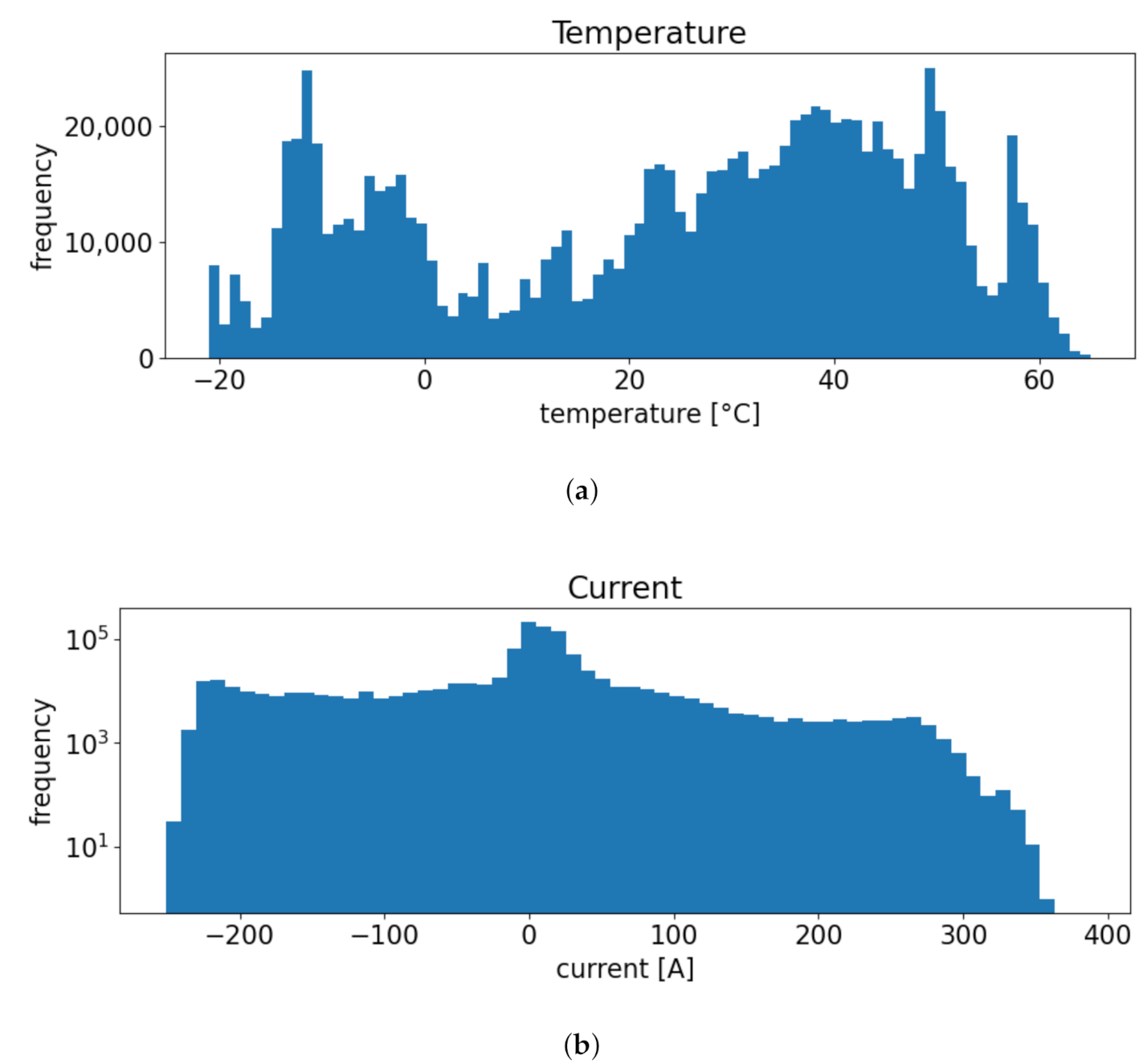
The noise range was set from −2 to 2 °C in 1 °C steps, such that every under-represented data point was quintupled. The final data distribution can be seen in Figure 2. The current was almost equally distributed, except in two areas. Very low and very high currents were still under-represented, due to the fact that the system rarely operates in these areas. The range around zero current was over-represented, which was due to some rest periods. Undersampling this area would lead to an inability to perceive the open-circuit voltage (OCV). Due to warming in the battery during operation, there were many more data for higher temperatures than for lower.

3.2.3. Normalizing

The different ranges of the input features need to be normalized, in order to improve numerical stability and to accelerate the training process. To avoid an oscillating or exploding loss with non-normalized data, a very small learning rate needs to be applied. This is caused by a non-symmetric cost function.

The feature with the largest range determines the learning rate. If the features are normalized, each feature is in the same range, leading to a higher learning rate. This speeds up the training process. A min–max scaler, as shown in Equation (13), was implemented for the proposed model, as it was considered the most effective scaling method.

$$\begin{array}{cc}\hfill \widehat{X}[:,i]& =\frac{X[:,i]-min\left(X\right[:,i\left]\right)}{max\left(X\right[:,i\left]\right)-min\left(X\right[:,i\left]\right)}.\hfill \end{array}$$

(13)

3.2.4. Sequentializing

Recurrent neural networks, such as GRUs or LSTMs, are built using sequence data as input. The sequence length is the same length as the section on which the model can fit the behavior. The lengths of sequences have a direct effect on the memory and speed necessary for computation. Considering that battery effects are highly time-dependent, a long sequence length is desirable. The internal effects of diffusion, charge transfer, electrochemical double layer and conductance have different time dependencies. Time constants for modeling these effects range from milliseconds to hours and are dependent on the SOC and temperature.

As a trade-off between computational cost and model accuracy, the sequence length was chosen as 128 data points. Data were logged with a sampling rate of 10 Hz, which means that each sequence represents the last 12.8 s of recording. Sequentializing was performed with a shift of one-step, such that no information was lost.

4. Battery Modeling and Rnn Hyperparameter Tuning

Selecting a smart input feature enables simple utilization in vehicle applications. The model accuracy is highly dependent on the chosen hyperparameters and model architectures.

4.1. Feature Selection

Input feature selection has a significant influence on the convergence of ML models. Battery voltage prediction models are often trained with the terminal current, battery temperature, actual voltage and an indicator of the remaining capacity, such as the SOC or a similar charge counter. Due to the computational cost and inaccuracy of SOC modeling, the proposed model was trained without SOC as an input feature. To bypass the issue of modeling the SOC, some current integration methods have been applied in the literature. The side effect of this is that either the initial SOC or some extra information about the battery state must be known, such as whether the battery is fully charged or fully discharged. This extra information and current integration over time provides a kind of SOC to the net.

The operation strategy of a 48 V system in automotive applications pre-defines a volatile battery operating area. With rarely stationary states, an adaptable model has to be designed. Therefore, the input features of the model were selected as:

• Terminal current $I_t$,
• Temperature $T_t$,
• Terminal voltage $U_t$, and
• Voltage trend $U_{trend}$.

Table 2. Prediction scheme with sequence length of ten.

Step	T	I	Utrend	U
0	T0	I0	Umean(U0:U8)	U0
1	T1	I1	Umean(U0:U8)	U1
2	T2	I2	Umean(U0:U8)	U2
3	T3	I3	Umean(U0:U8)	U3
4	T4	I4	Umean(U0:U8)	U4
5	T5	I5	Umean(U0:U8)	U5
6	T6	I6	Umean(U0:U8)	U6
7	T7	I7	Umean(U0:U8)	U7
8	T8	I8	Umean(U0:U8)	U8
9	T9	I9	Umean(U0:U8)	Upred

shows an exemplary sequence (with a sequence length of 10) for the target value $U_{pred}$ and the corresponding input features. The calculation of $U_{trend}$ contains no new information, but, as an input, it ensures faster and more precise convergence when training the model. The average voltage over the last few steps provides information about which voltage level the battery is actually operating at. Furthermore, when combined with the previous current and voltage, it can provide the trend of overvoltage polarization. The current and temperature determine the overvoltage polarization in the next step. When predicting more than one step at once, the $U_{trend}$ is recalculated every minute by using the last sequence of predicted voltages. Use of the period of 60 s ensures that small errors in voltage prediction are not fed directly to the next step as input. Updating $U_{trend}$ in every iteration could result in a drift of voltage and, therefore, an increasing error.

The input feature set used provides all of the information needed for learning, whereby the future voltages of a battery can be predicted. This approach has two advantages: First, explicit battery modeling knowledge from experts is not necessary to model the behavior. Feature selection and hyperparameter tuning are implemented and can be adapted to any lithium-ion battery by simple data preparation and model adjustments. Second, an online algorithm is provided which is applicable in every condition during operation, with a short initializing time for the sequence length.

4.2. Training Progress

The input data obtained from the pre-processing steps were divided into batches, in order to reduce the memory size required for each training iteration. An epoch is considered complete when every batch has been processed once in an iteration. Figure 3a shows the loss and Figure 3b shows the validation loss over the trained epochs. As the loss decreases steadily, the model keeps on learning the input data inter-relations. Overfitting is indicated by an increasing validation loss beyond Epoch 60. The loss metrics of the test set had their lowest point in Epoch 35.

4.3. Proposed Model Architecture

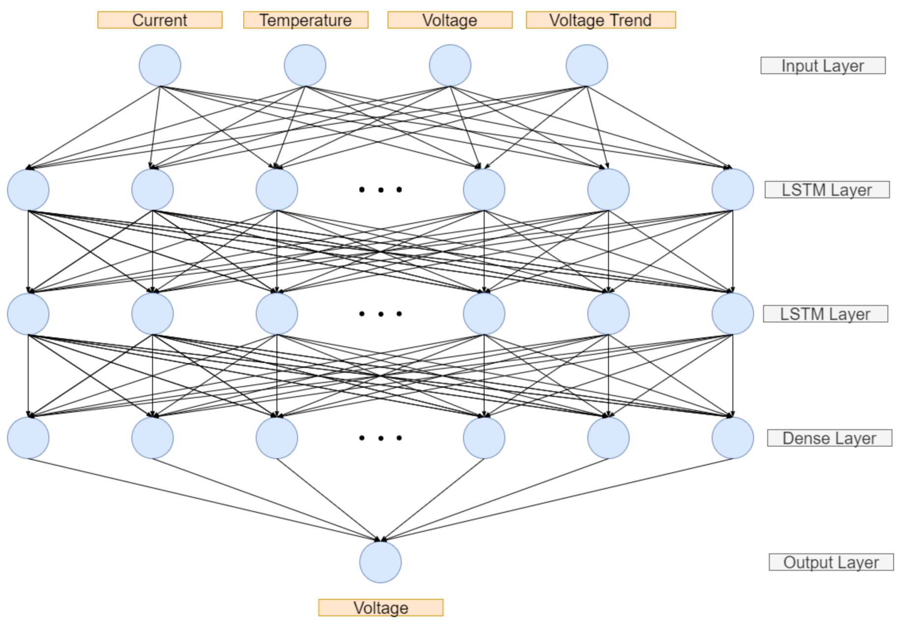
The input and output layers of the neural net were determined by the feature selection and sequence length, as shown in Figure 4. This approach used four features with a sequence length of 128 and, thus, the input of the first layer was a 128 × 4 matrix for each time step. The output was simply the predicted voltage for the next step.

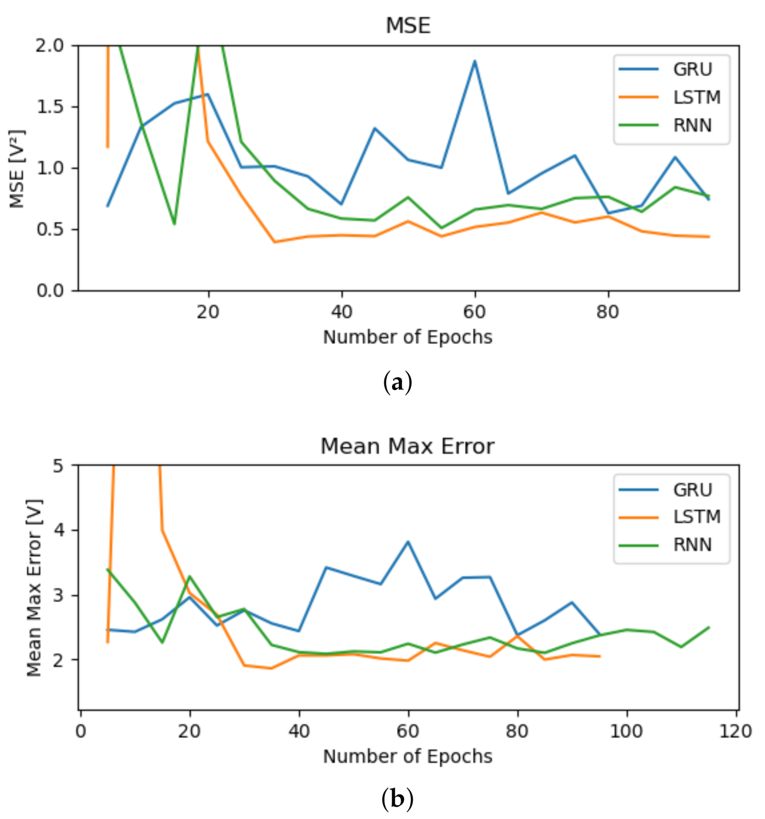
Figure 5 demonstrates that the LSTM cells had better validation results, compared to those of the RNN and GRU. From Epoch 30 onwards, the LSTM had lower MSE and performed slightly better than the RNN, with regard to the mean max error. In addition, the training time per epoch was three times faster when using the LSTM, compared to the RNN, and similar to that of the GRU. The hidden layers were determined empirically as two LSTM layers with 128 neurons each and one attached dense layer with 128 neurons. An additional dropout layer with a dropout rate of 0.2 was also used, in order to deal with overfitting issues. The model hyperparameters shown in

Table 3. Network hyperparameters.

Hyperparameter	Value
Number of LSTM layers	2
Number of dense layers	1
Units per layer	128
Dropout rate	0.2
Learning rate	0.0002
Number of epochs	100
Batch size	1024
Optimizer	Adam
Loss function	MSE
Sequence length	128

were determined empirically for the proposed models using a grid search algorithm.

The model was trained on an NVIDIA RTX 2080 Ti GPU with 1350 MHz clock speed and 11 GB RAM using the TensorFlow backend. Every model architecture was trained for at least 100 epochs, where one epoch lasted about 60 s, depending on the number of layers and neurons. Full test validation would be very time intensive and, thus, test validation was only performed after every fifth epoch with the test set.

5. Validation Using Test Bench Measurements

A comparison between the model prediction and test bench measurements was carried out, in order to validate the proposed model. The error was quantified by calculating the MAE and MSE, as described in Equations (15) and (16), respectively. The error at each step, $err\left(t\right)$, was calculated using the ground truth $gt\left(t\right)$ and the predicted values from the model $pre{d}_{model}\left(t\right)$. n describes the number of steps.

$$\begin{array}{cc}\hfill err\left(t\right)& =gt\left(t\right)-pre{d}_{model}\left(t\right)\hfill \end{array}$$

(14)

$$\begin{array}{cc}\hfill MAE& =\frac{{\sum }_{t=1}^n\left|err\left(i\right)\right|}{n},\hfill \end{array}$$

(15)

$$\begin{array}{cc}\hfill MSE& =\frac{{\sum }_{t=1}^n{\left|err\left(i\right)\right|}^2}{n}.\hfill \end{array}$$

(16)

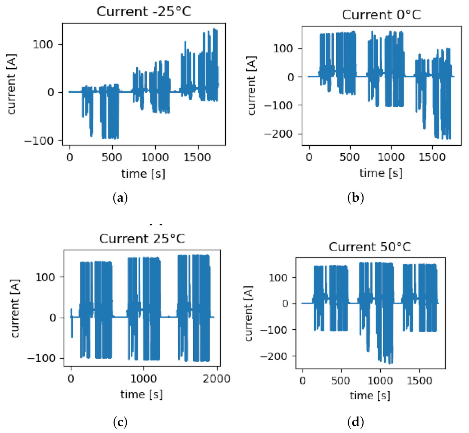
Unlike the training and validation datasets, the test set was measured on a test bench, where the temperature and current were adjustable. This ensured that a wide range of power, SOC and temperature could be tested. To achieve this, a current profile was recorded during a vehicle test drive and adapted to the adjusted temperature and SOC to obtain the voltage boundaries of the battery. Batteries display non-linear behavior in the SOC and voltage limit values, due to the steepening OCV and rising internal resistances. Adapting the current profiles allows access to these hard-to-predict areas, thus ensuring more exact validation. The test bench offers a measurement setup with a climate chamber to condition the battery temperature, a power supply and electric load to apply the current profiles and a computer to control the BMS and plot the data. Before starting measurement, the batteries were first conditioned electrically to the requested state of charge by completely discharging a fully charged battery. Thermal conditioning was then carried out for at least 12 h to ensure a fully tempered battery. Concatenated current profiles for the four temperature regions are shown in Figure 6. The current is selected to meet the requirements of the test-bench and voltage limits in consideration of temperature dependent overvoltages.

Figure 7 presents a validation of the current profile applied at an average temperature of −23 °C in low SOC regions. The validation had difficulties predicting these operation points. As Figure 7a shows, the model was nevertheless capable of predicting the qualitative progression of the voltage with an MSE of 1.18 V². The prediction differed from the ground truth at high rates due to the gradient of inner resistances in the battery cell increasing at lower temperatures. Figure 7b shows the maximum error (of 3.9 V) occurring during a high current peak.

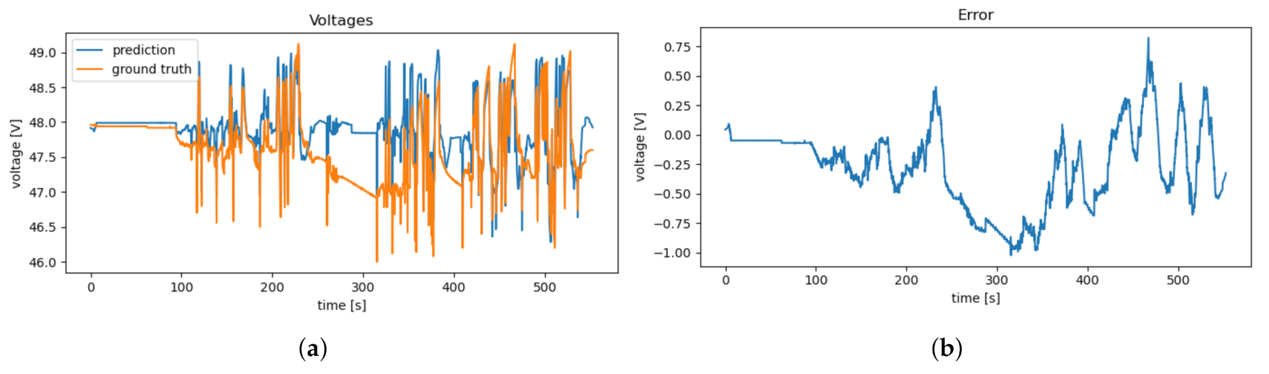
The better voltage prediction closer to room temperature is shown in Figure 8a. The maximum error was less than 1.1 V with an MSE of 0.19 V² within this profile, as shown in Figure 8b. Better predictions resulted from a less volatile voltage course and more resilient data availability. This temperature-dependent error is similar to that occurring in common ECMs.

Three different current profiles were performed at different charge states for every temperature region. The maximum and minimum current were restricted at −25 °C, such that the lower and upper voltage barriers of 38 and 53 V were not exceeded. There was no current restriction at 25 °C, on account of the lower inner resistance. The measured profiles were used as the input for the prediction, in order to obtain an equivalent input profile for validation. The model predicted current and temperature, where the first 128 voltage values were used to calculate the initial $U_{trend}$. $U_{trend}$ was then updated every 60 s and was calculated in consideration of the last 128 predicted voltage values.

Each adapted profile was evaluated individually, in order to determine the deficiencies of the model. As regards the voltage level of 48 V, the overall maximum relative error is below 1% at all conditions. The error metrics are summarized in

Table 4. Validation errors of the test set profiles.

Profile	MAE [V]	MaxError [V]	MSE [V2]	Mean Temp [°C]	Mean Voltage [V]
1	0.734785	2.963551	0.818735	−2.578630	44.894085
2	0.345099	1.590984	0.291348	−17.880545	45.090210
3	0.221103	1.251659	0.108364	−17.000000	47.619461
4	0.430389	2.482880	0.343608	−0.494065	43.953995
5	0.611864	2.738808	0.712661	1.473041	43.313877
6	0.308964	1.174629	0.162599	53.152065	43.104599
7	0.402310	1.196079	0.249962	56.111210	44.732620
8	0.339628	1.021107	0.187283	27.318338	47.641869
9	0.321065	1.027824	0.169096	29.902288	44.442562
10	0.498891	1.313484	0.403387	31.953856	42.876999
11	0.365947	1.216549	0.223687	48.910248	46.265839
12	0.678125	3.916935	1.175681	−23.398380	44.776375
Mean	0.438181	1.82454	0.403868	15.6225	44.8927

.

6. Conclusions

A novel battery modeling approach using an LSTM is proposed for a lithium-ion battery in vehicle applications. The calculated $U_{trend}$ and the balanced input dataset give the possibility to train a model without using the SOC and the included difficulties. Two steps were carried out to achieve a valid model: First, the raw experimental data were pre-processed to obtain a useful input vector. With under- and oversampling, redundant data were reduced and under-represented areas were reproduced, respectively. Sequentializing and normalizing permitted adequate training. Second, hyperparameter tuning was carried out during training, in order to find the optimal model architecture. Validation showed that the model accuracy was within an appropriate range. The maximum error in the validation set was below 1% (or 3.9 V) with an MSE of 0.40 V² over a Temperature range from −23 to 56 °C and power up to 11 kW.

The proposed battery model can be used in real-time applications, as the model inputs are physically measurable parameters. This ensures the possibility of simple and accurate implementation in a BMS. Its accuracy and transferability to other battery types mean that the developed modeling method can be used in a variety of mild-hybrid vehicles.

Future work may involve battery SOP estimation based on the proposed voltage prediction. A more robust voltage prediction in the peripheral SOC areas must, thus, be trained.

References

- Mark, S.; Christian, S.; Ferit, K. The Potential of 48V HEV in Real Driving. In Proceedings of the 17th International Conference on Hybrid and Electric Vehicles, Osaka, Japan, 15–18 December 2015. [Google Scholar] [CrossRef]
- Liu, Z.; Ivanco, A.; Filipi, Z.S. Impacts of Real-World Driving and Driver Aggressiveness on Fuel Consumption of 48V Mild Hybrid Vehicle. SAE Int. J. Altern. Powertrains 2016, 5, 249–258. [Google Scholar] [CrossRef]
- Ranjbar, A.H.; Banaei, A.; Khoobroo, A.; Fahimi, B. Online Estimation of State of Charge in Li-Ion Batteries Using Impulse Response Concept. IEEE Trans. Smart Grid 2012, 3, 360–367. [Google Scholar] [CrossRef]
- Chiang, Y.H.; Sean, W.Y.; Ke, J.C. Online estimation of internal resistance and open-circuit voltage of lithium-ion batteries in electric vehicles. J. Power Sources 2011, 196, 3921–3932. [Google Scholar] [CrossRef]
- Madani, S.; Schaltz, E.; Knudsen Kær, S. An Electrical Equivalent Circuit Model of a Lithium Titanate Oxide Battery. Batteries 2019, 5, 31. [Google Scholar] [CrossRef]
- Hu, X.; Li, S.E.; Yang, Y. Advanced Machine Learning Approach for Lithium-Ion Battery State Estimation in Electric Vehicles. IEEE Trans. Transp. Electrif. 2016, 2, 140–149. [Google Scholar] [CrossRef]
- Charkhgard, M.; Farrokhi, M. State-of-Charge Estimation for Lithium-Ion Batteries Using Neural Networks and EKF. IEEE Trans. Ind. Electron. 2010, 57, 4178–4187. [Google Scholar] [CrossRef]
- Chemali, E.; Kollmeyer, P.J.; Preindl, M.; Emadi, A. State-of-charge estimation of Li-ion batteries using deep neural networks: A machine learning approach. J. Power Sources 2018, 400, 242–255. [Google Scholar] [CrossRef]
- Yang, F.; Song, X.; Xu, F.; Tsui, K.L. State-of-Charge Estimation of Lithium-Ion Batteries via Long Short-Term Memory Network. IEEE Access 2019, 7, 53792–53799. [Google Scholar] [CrossRef]
- Khalid, A.; Sundararajan, A.; Acharya, I.; Sarwat, A.I. Prediction of Li-Ion Battery State of Charge Using Multilayer Perceptron and Long Short-Term Memory Models. In Proceedings of the IEEE Transportation Electrification Conference and Expo (ITEC), Novi, MI, USA, 19–21 June 2019; pp. 1–6. [Google Scholar] [CrossRef]
- Li, C.; Xiao, F.; Fan, Y. An Approach to State of Charge Estimation of Lithium-Ion Batteries Based on Recurrent Neural Networks with Gated Recurrent Unit. Energies 2019, 12, 1592. [Google Scholar] [CrossRef]
- Yang, F.; Li, W.; Li, C.; Miao, Q. State-of-charge estimation of lithium-ion batteries based on gated recurrent neural network. Energy 2019, 175, 66–75. [Google Scholar] [CrossRef]
- Huang, Z.; Yang, F.; Xu, F.; Song, X.; Tsui, K.L. Convolutional Gated Recurrent Unit–Recurrent Neural Network for State-of-Charge Estimation of Lithium-Ion Batteries. IEEE Access 2019, 7, 93139–93149. [Google Scholar] [CrossRef]
- Vidal, C.; Malysz, P.; Kollmeyer, P.; Emadi, A. Machine Learning Applied to Electrified Vehicle Battery State of Charge and State of Health Estimation: State-of-the-Art. IEEE Access 2020, 8, 52796–52814. [Google Scholar] [CrossRef]
- Sepasi, S.; Ghorbani, R.; Liaw, B.Y. Improved extended Kalman filter for state of charge estimation of battery pack. J. Power Sources 2014, 255, 368–376. [Google Scholar] [CrossRef]
- Meng, J.; Boukhnifer, M.; Diallo, D.; Wang, T. A New Cascaded Framework for Lithium-Ion Battery State and Parameter Estimation. Appl. Sci. 2020, 10, 1009. [Google Scholar] [CrossRef]
- You, G.w.; Park, S.; Oh, D. Real-time state-of-health estimation for electric vehicle batteries: A data-driven approach. Appl. Energy 2016, 176, 92–103. [Google Scholar] [CrossRef]
- Chaoui, H.; Ibe-Ekeocha, C.C. State of Charge and State of Health Estimation for Lithium Batteries Using Recurrent Neural Networks. IEEE Trans. Veh. Technol. 2017, 66, 8773–8783. [Google Scholar] [CrossRef]
- Zhang, C.; Zhu, Y.; Dong, G.; Wei, J. Data-driven lithium-ion battery states estimation using neural networks and particle filtering. Int. J. Energy Res. 2019, 43, 3681. [Google Scholar] [CrossRef]
- Zhao, R.; Kollmeyer, P.J.; Lorenz, R.D.; Jahns, T.M. A Compact Methodology Via a Recurrent Neural Network for Accurate Equivalent Circuit Type Modeling of Lithium-Ion Batteries. IEEE Trans. Ind. Appl. 2019, 55, 1922–1931. [Google Scholar] [CrossRef]
- Lippmann, R. An introduction to computing with neural nets. IEEE ASSP Mag. 1987, 4, 4–22. [Google Scholar] [CrossRef]
- Goodfellow, I.; Bengio, Y.; Courville, A. Deep Learning; MIT Press: Cambridge, MA, USA; London, UK, 2016. [Google Scholar]
- Nitish, S.; Geoffrey, H.; Alex, K.; Ilya, S.; Ruslan, S. Dropout: A Simple Way to Prevent Neural Networks from Overfitting. J. Mach. Learn. Res. 2014, 15, 1929–1958. [Google Scholar]
- Cho, K.; van Merrienboer, B.; Gulcehre, C.; Bahdanau, D.; Bougares, F.; Schwenk, H.; Bengio, Y. Learning Phrase Representations using RNN Encoder-Decoder for Statistical Machine Translation. arXiv 2014, arXiv:1406.1078. [Google Scholar]
- Hochreiter, S.; Schmidhuber, J. Long short-term memory. Neural Comput. 1997, 9, 1735–1780. [Google Scholar] [CrossRef]
- Liu, S.; Jiang, J.; Shi, W.; Ma, Z.; Le Wang, Y.; Guo, H. Butler-Volmer-Equation-Based Electrical Model for High-Power Lithium Titanate Batteries Used in Electric Vehicles. IEEE Trans. Ind. Electron. 2015, 62, 7557–7568. [Google Scholar] [CrossRef]
- Feng, T.; Yang, L.; Zhao, X.; Zhang, H.; Qiang, J. Online identification of lithium-ion battery parameters based on an improved equivalent-circuit model and its implementation on battery state-of-power prediction. J. Power Sources 2015, 281, 192–203. [Google Scholar] [CrossRef]
- Hussein, A.A.H.; Batarseh, I. An overview of generic battery models. In Proceedings of the 2011 IEEE Power and Energy Society General Meeting, Detroit, MI, USA, 24–29 July 2011; pp. 1–6. [Google Scholar] [CrossRef]
- Nikolian, A.; de Hoog, J.; Fleurbaey, K.; Timmermans, J.M.; Omar, N.; van den Bossche, P.; van Mierlo, J. Classification of Electric modeling and Characterization methods of Lithium-ion Batteries for Vehicle Applications. In Proceedings of the European Electric Vehicle Congress, Brussels, Belgium, 2–5 December 2014. [Google Scholar]
- Farmann, A.; Waag, W.; Sauer, D.U. Application-specific electrical characterization of high power batteries with lithium titanate anodes for electric vehicles. Energy 2016, 112, 294–306. [Google Scholar] [CrossRef]
- Kashkooli, A.G.; Fathiannasab, H.; Mao, Z.; Chen, Z. Application of Artificial Intelligence to State-of-Charge and State-of-Health Estimation of Calendar-Aged Lithium-Ion Pouch Cells. J. Electrochem. Soc. 2019, 166, A605–A615. [Google Scholar] [CrossRef]