Mechanism and Characteristics of Global Varying Compliance Parametric Resonances in a Ball Bearing

Abstract
1. Introduction
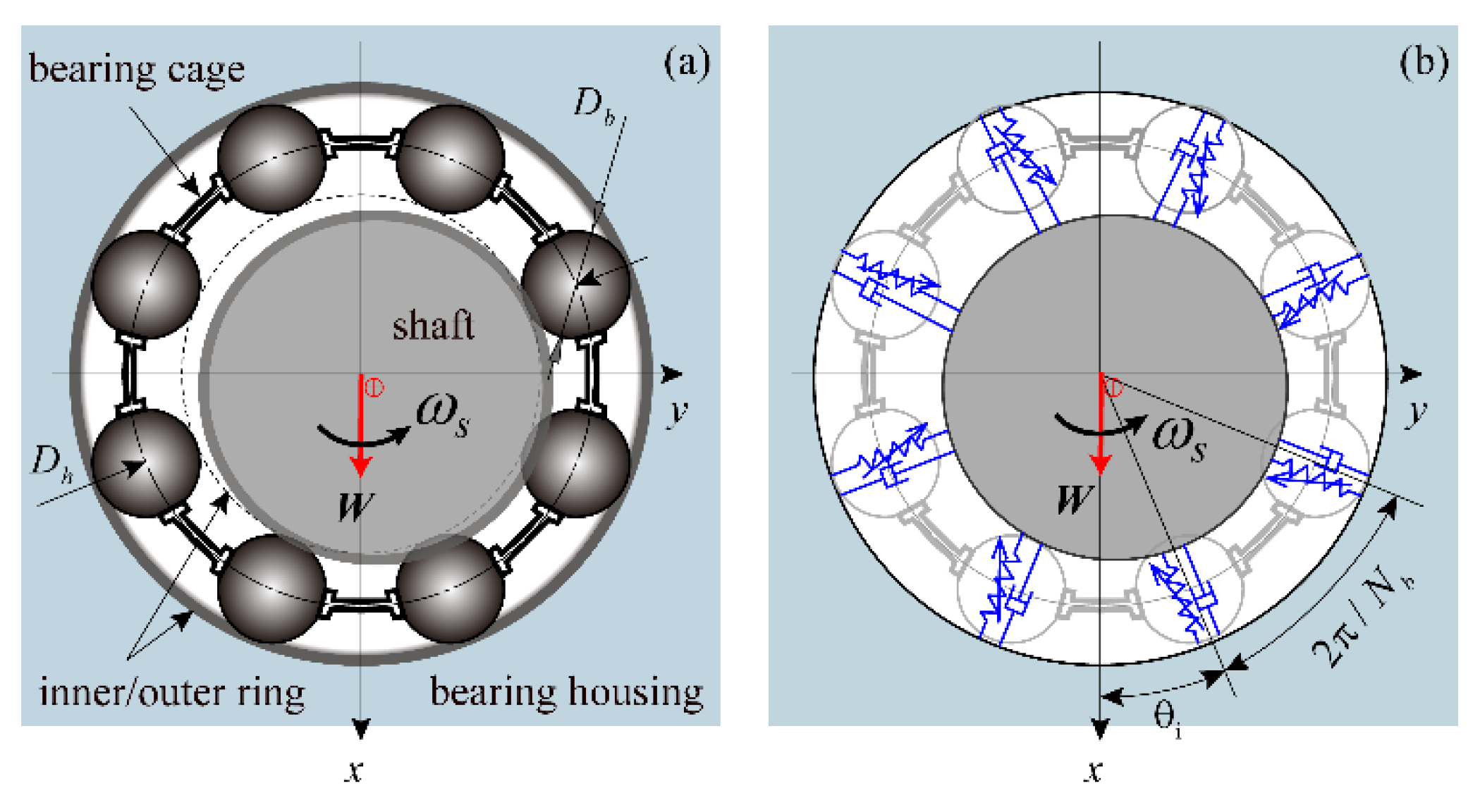
2. Description of Ball Bearing VC Vibration
3. Methodology
3.1. HB–AFT Method for Obtaining VC Period-M Solution
3.2. Floquet Stability Analysis of VC Period-M Solution
- A transcritical, symmetry-breaking, or cyclic-fold bifurcation may originate when the leading multiplier crosses through the unit circle at +1. Herein, the cyclic-fold bifurcation emerges only at the turning point of a solution branch.
- A period-doubling bifurcation occurs when the leading multiplier crosses the unit circle at −1.
- A secondary Hopf bifurcation occurs when a complex pair of multipliers moves out of the unit circle.
4. Results
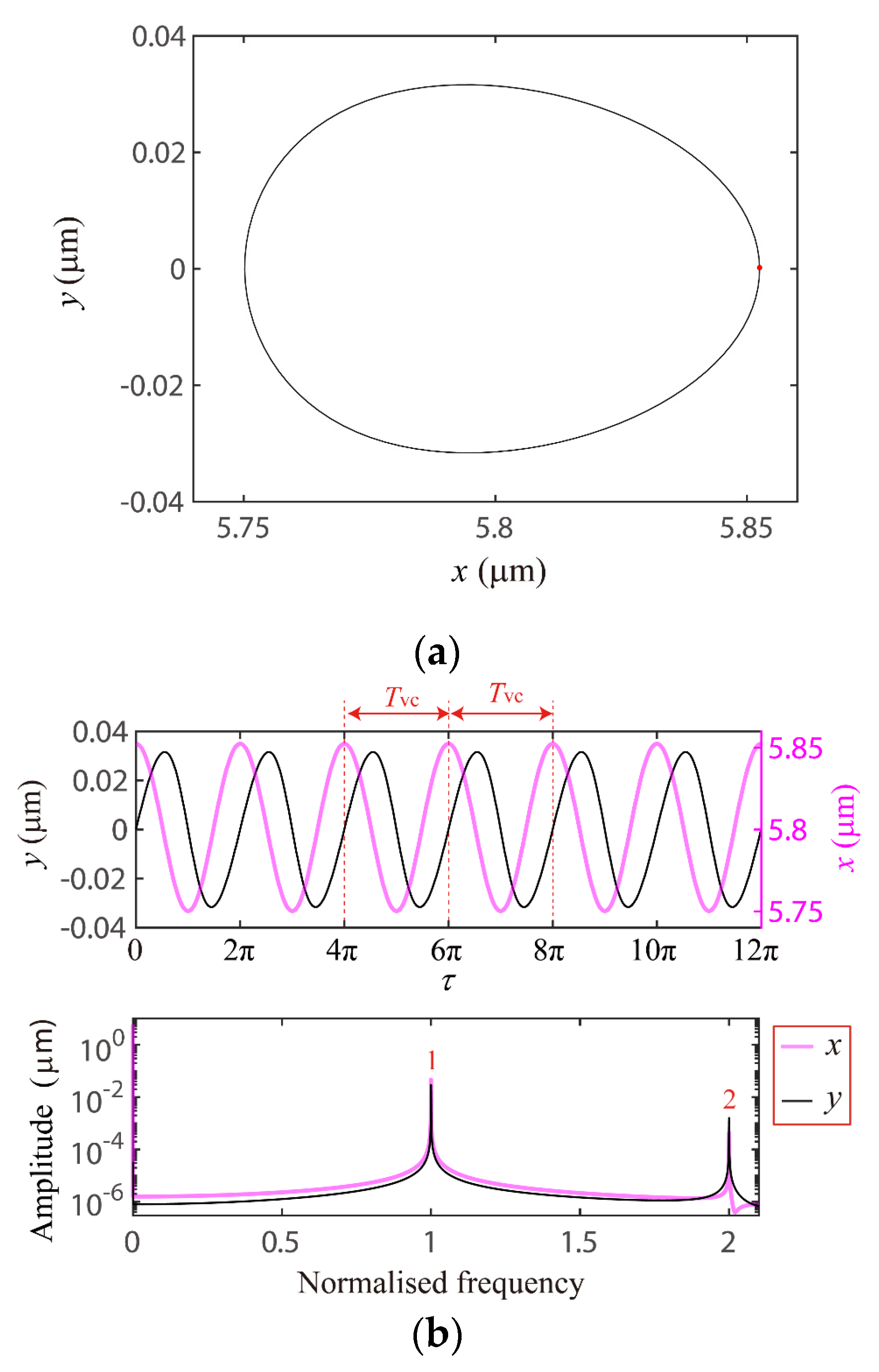
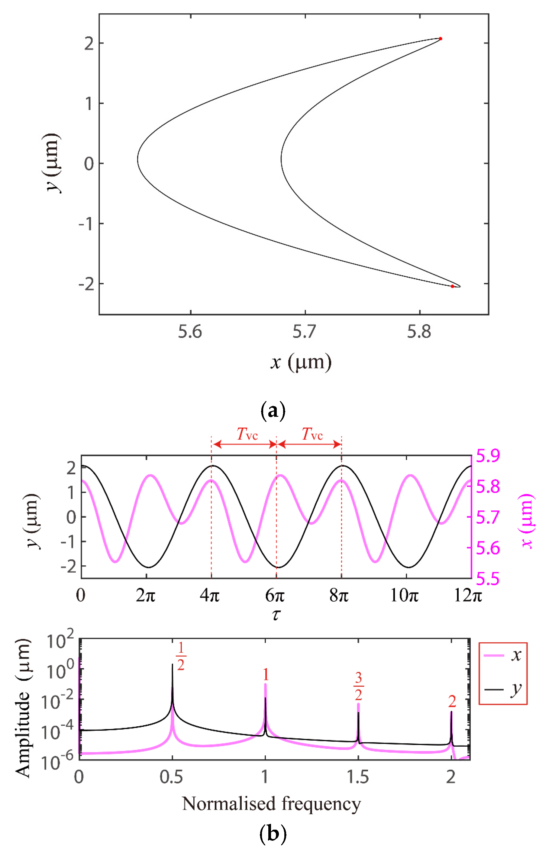
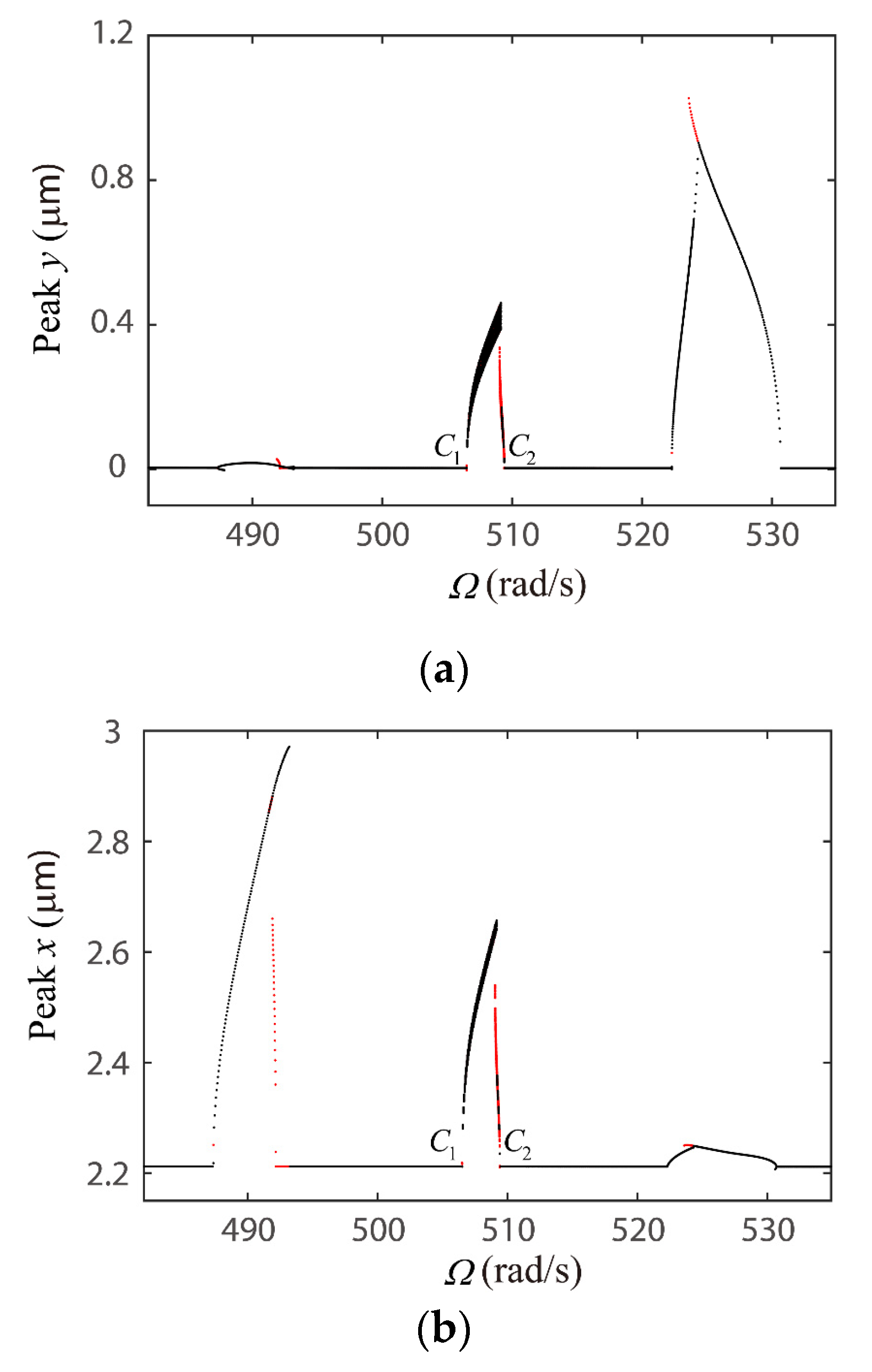
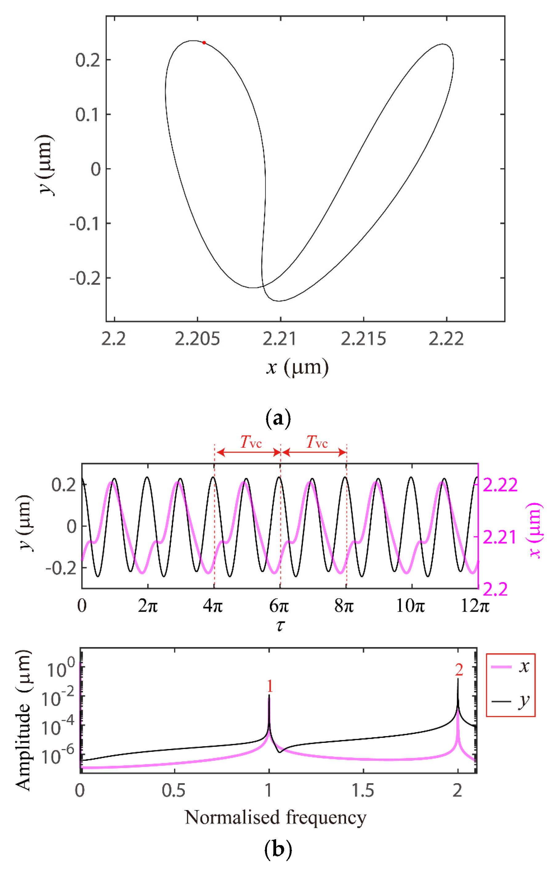
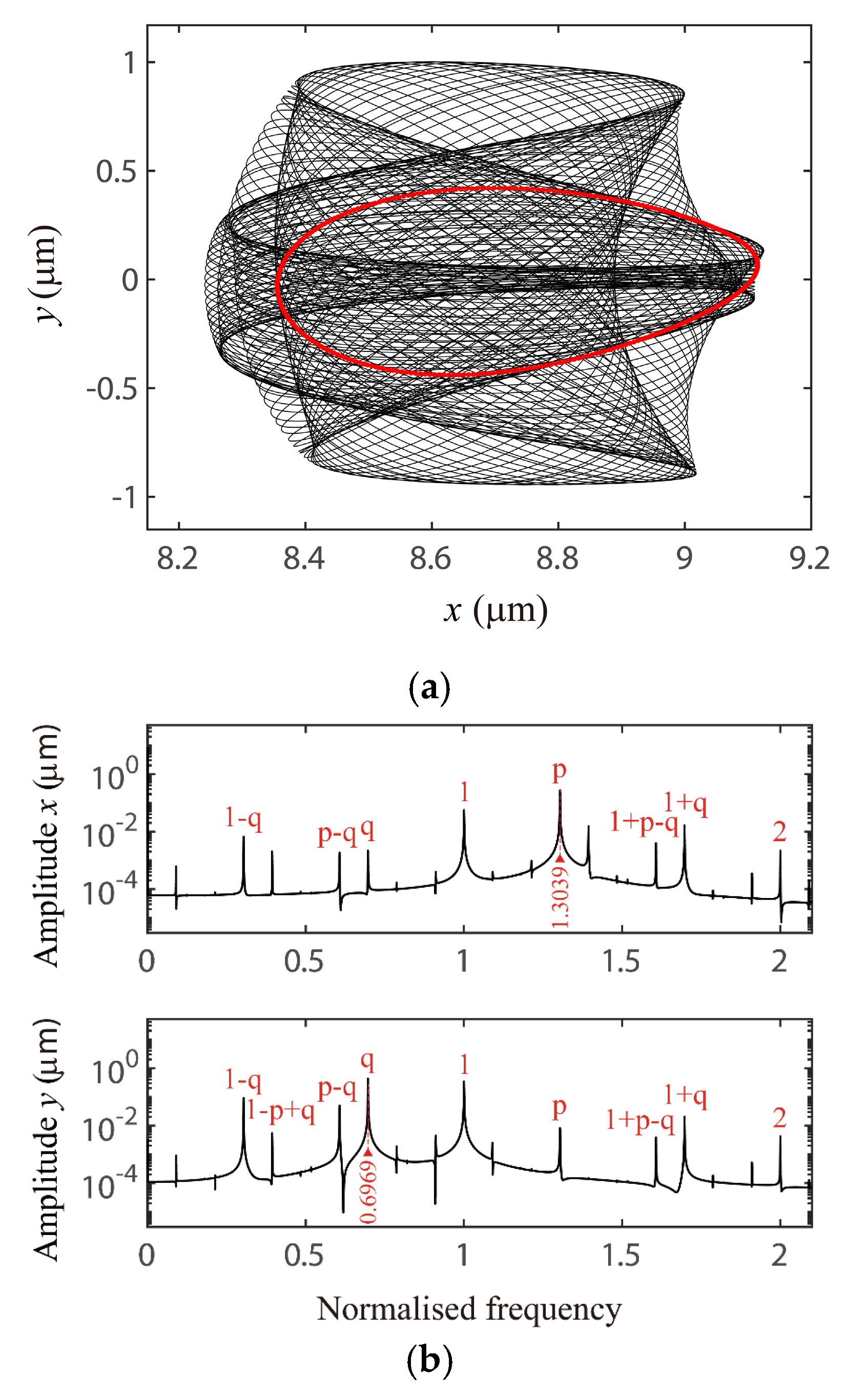
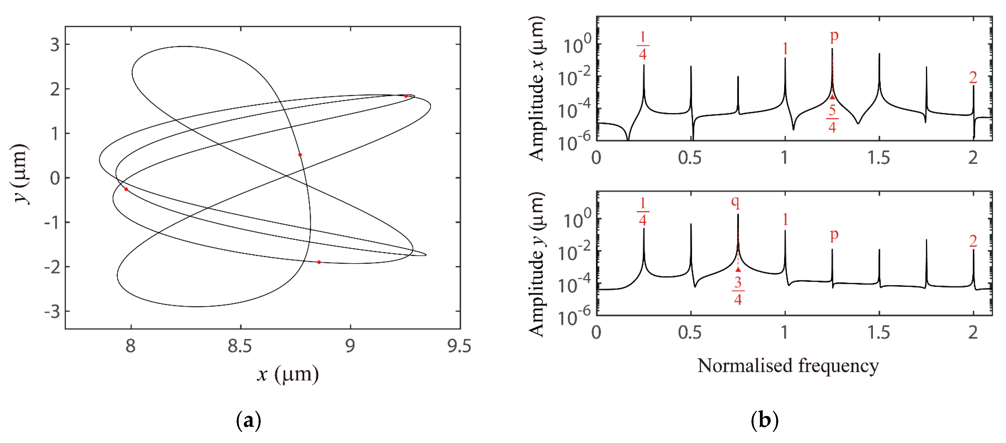
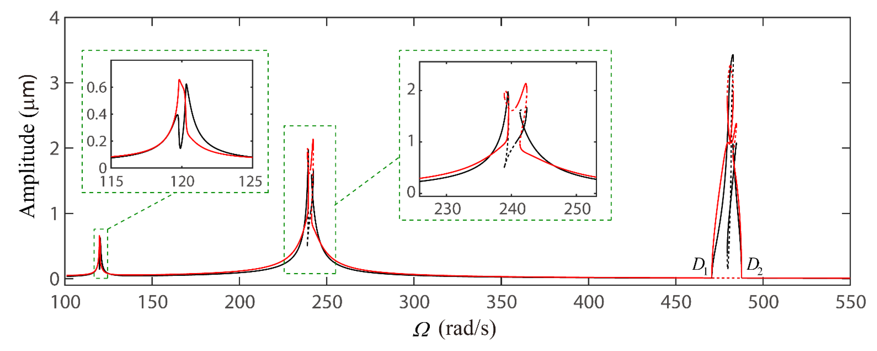
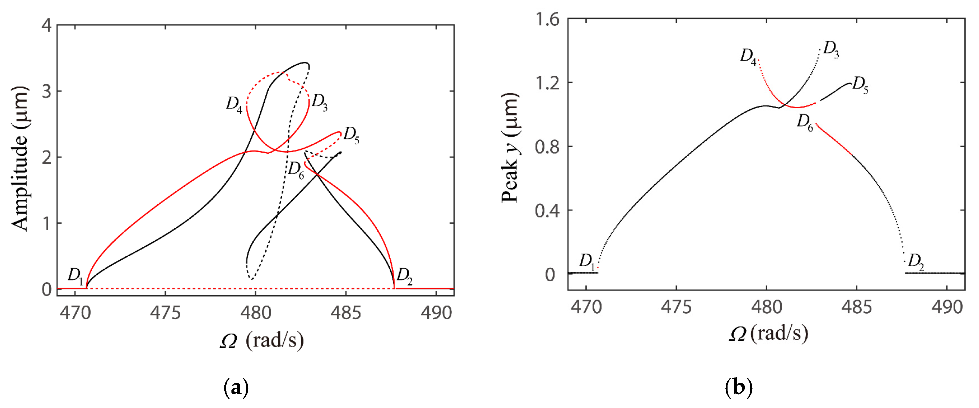
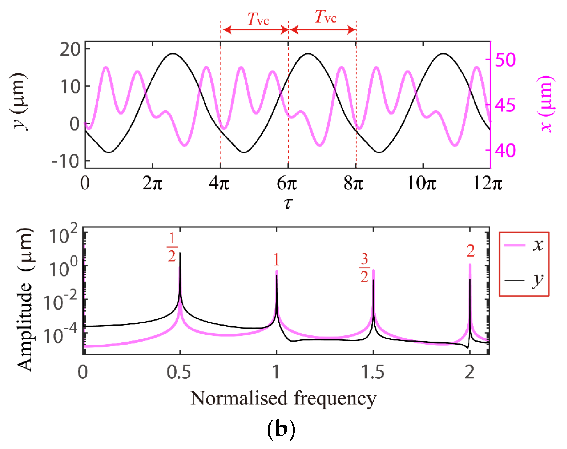
4.1. The VC 2-Order Superharmonc Resonance, 1/2-Order Subharmonic Resonance and the Case of ωx0 + ωy0 = Ωvc Combination Resonance
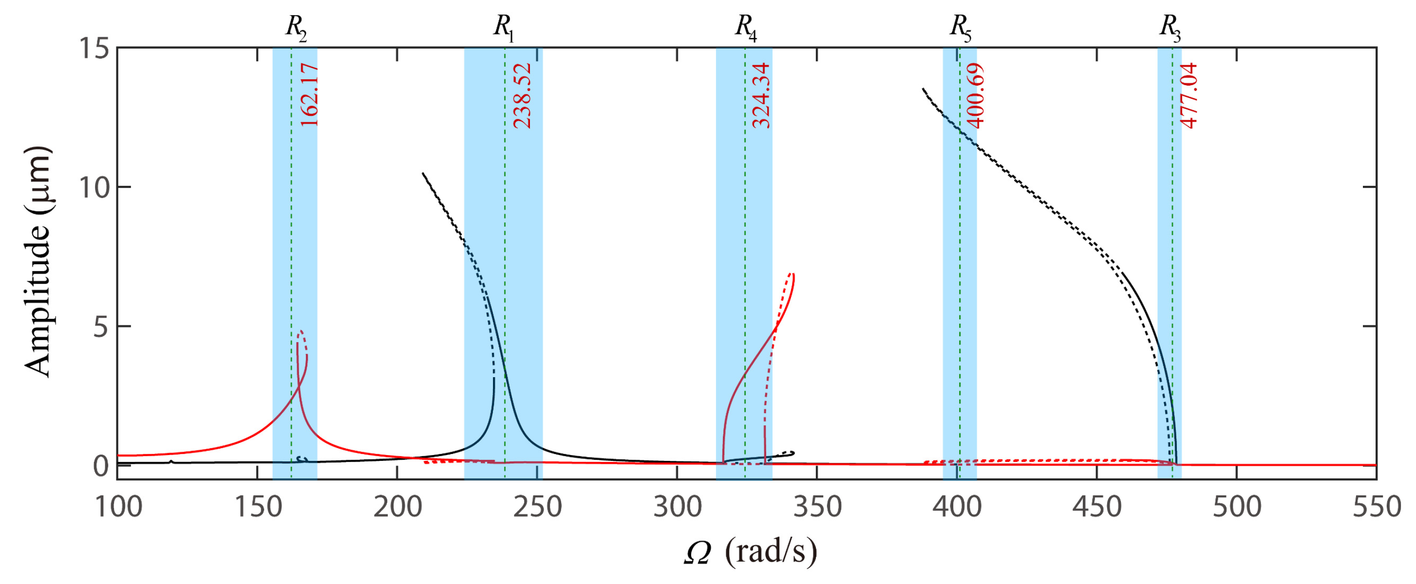
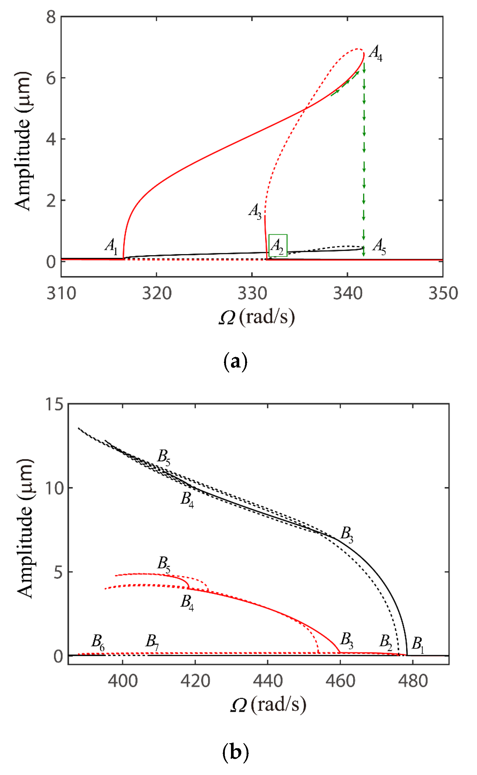
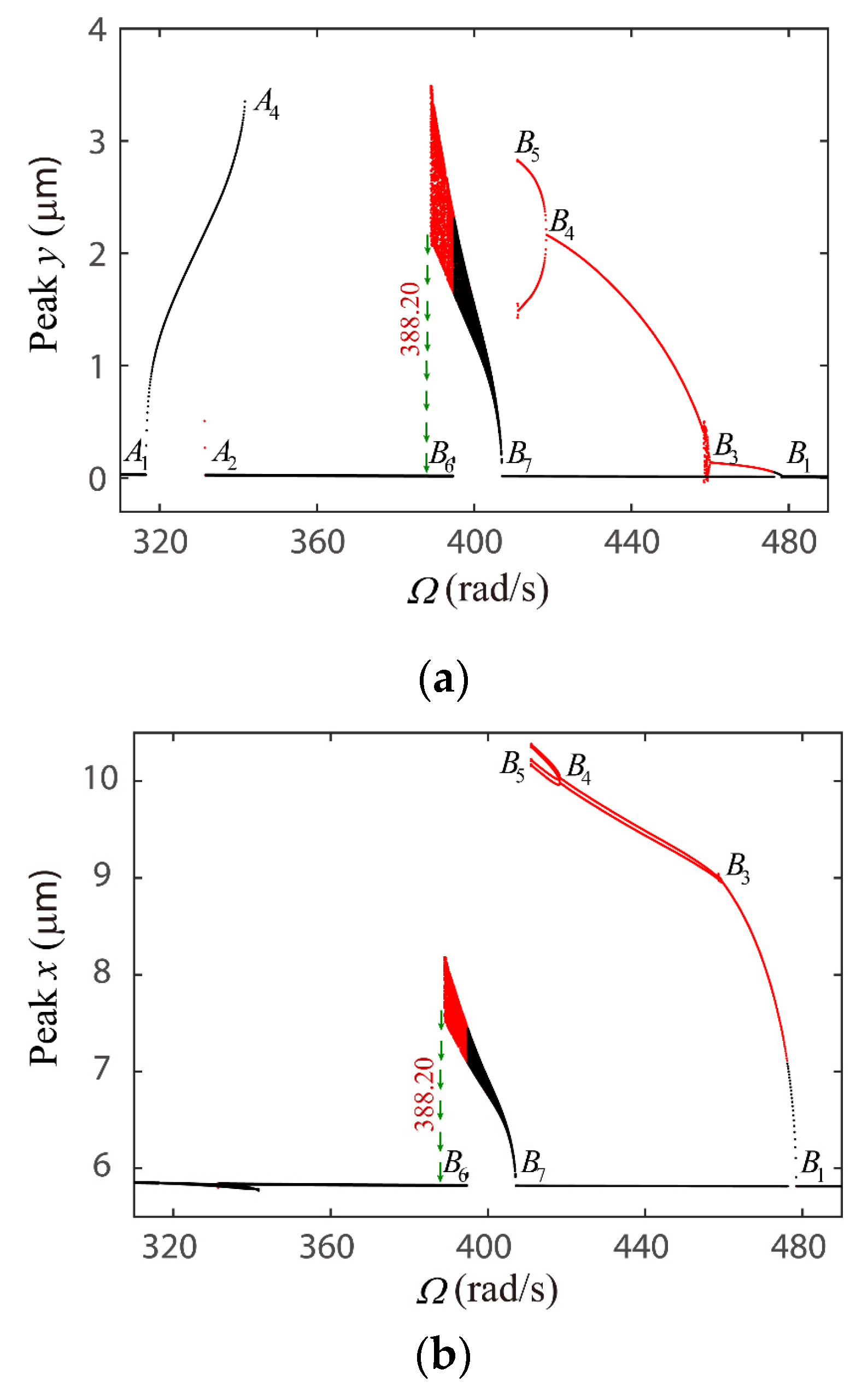
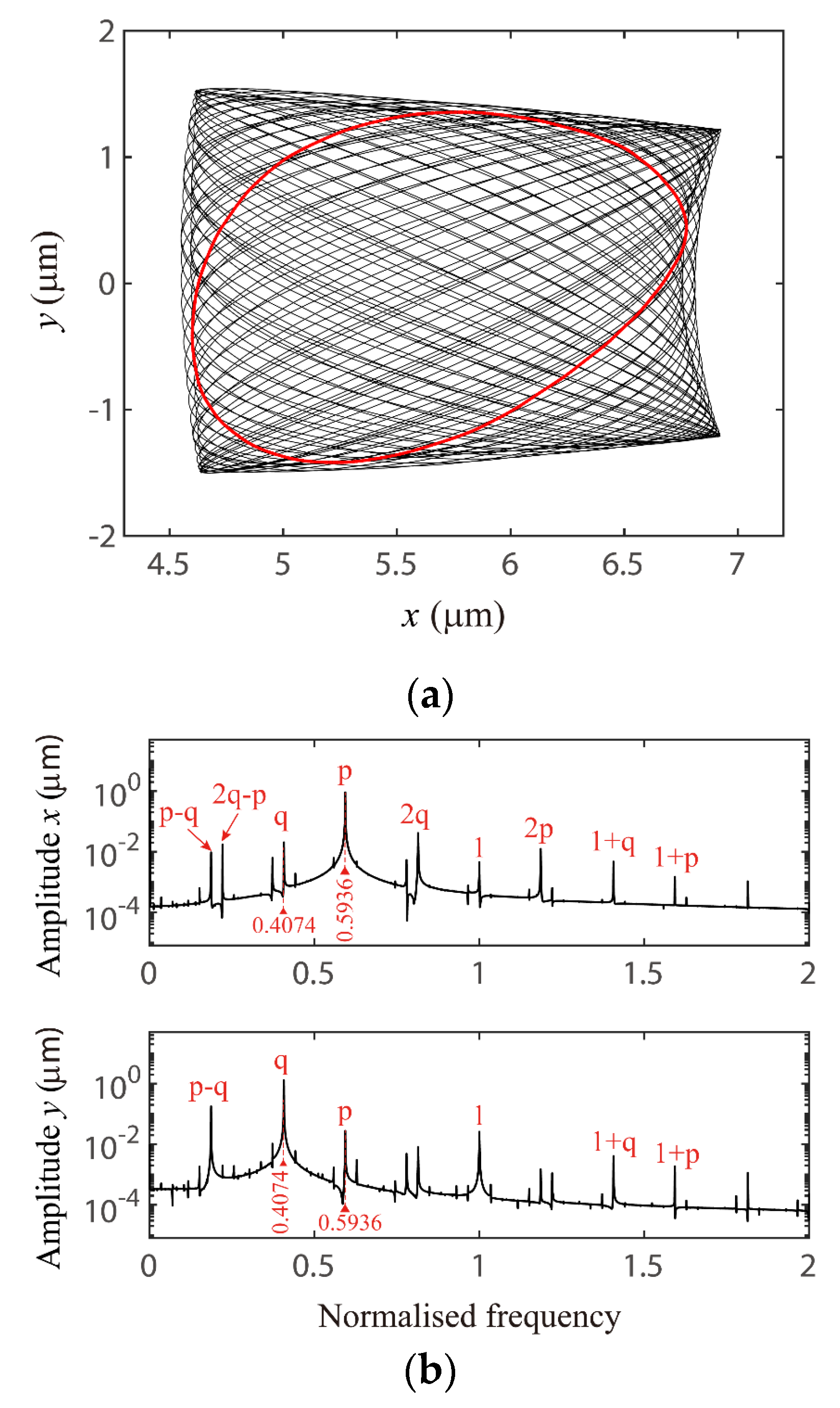
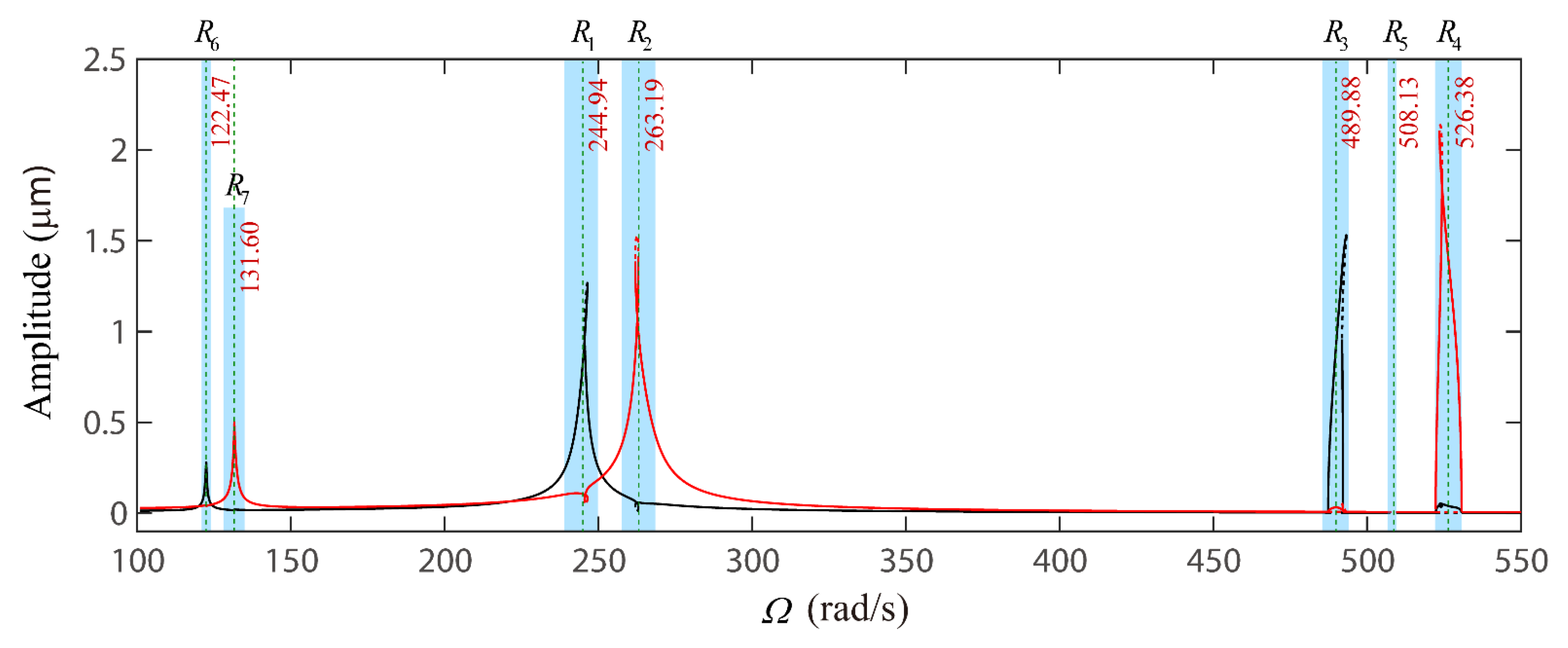
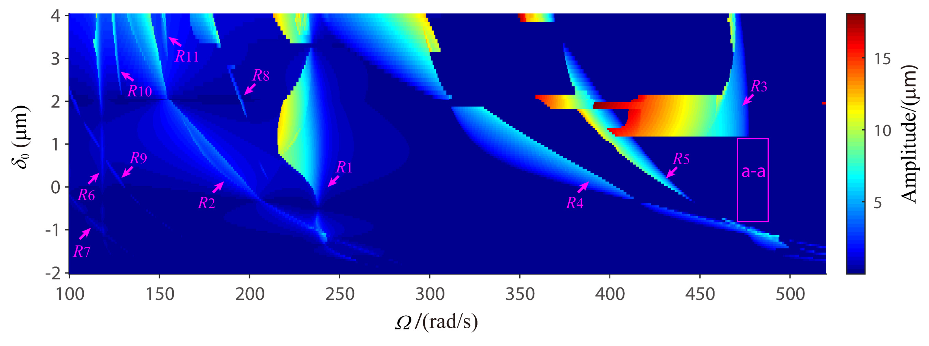
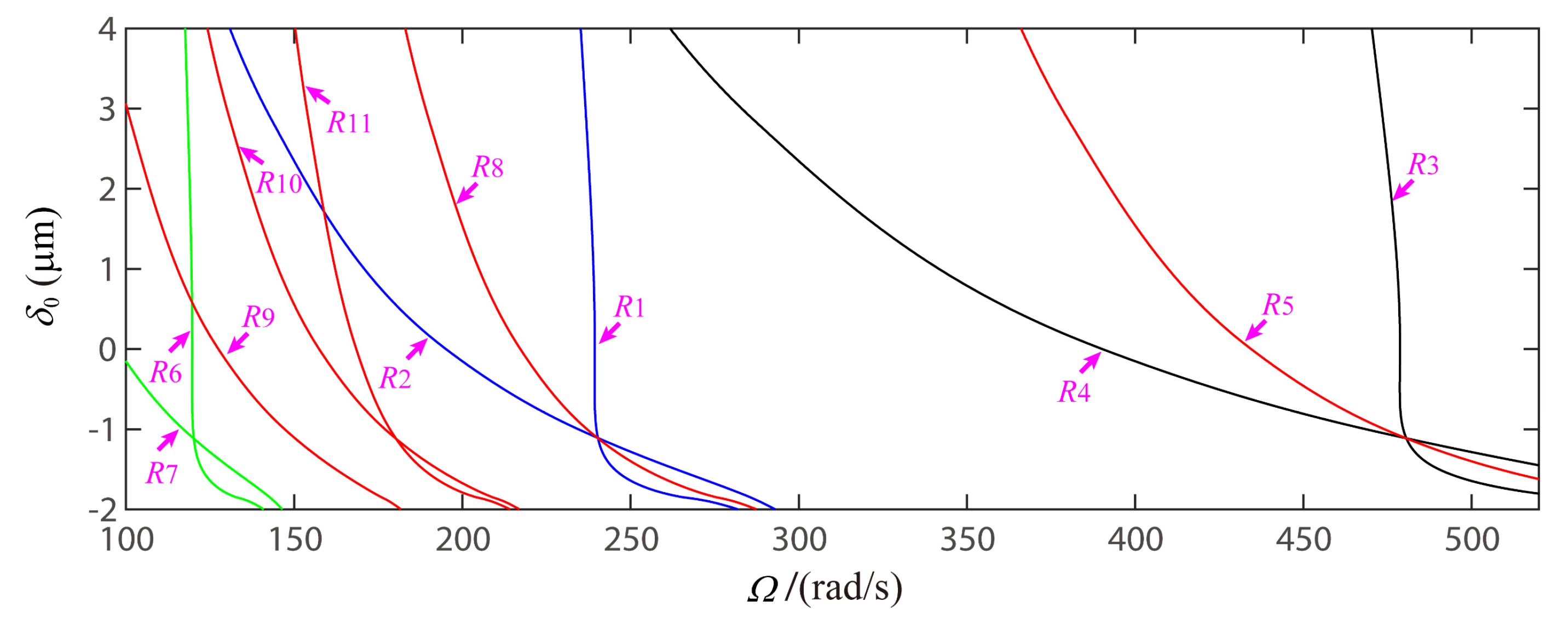
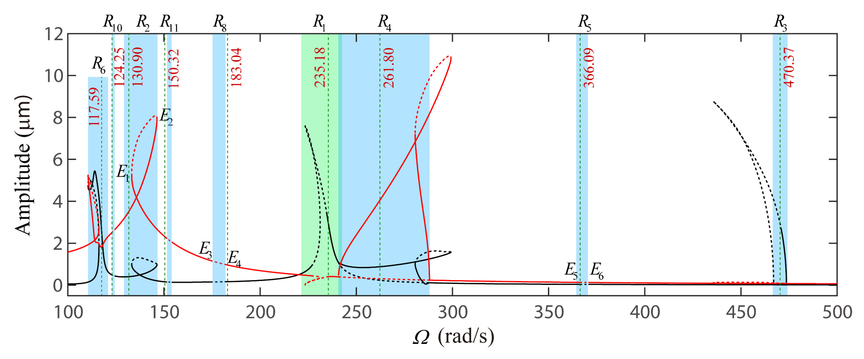
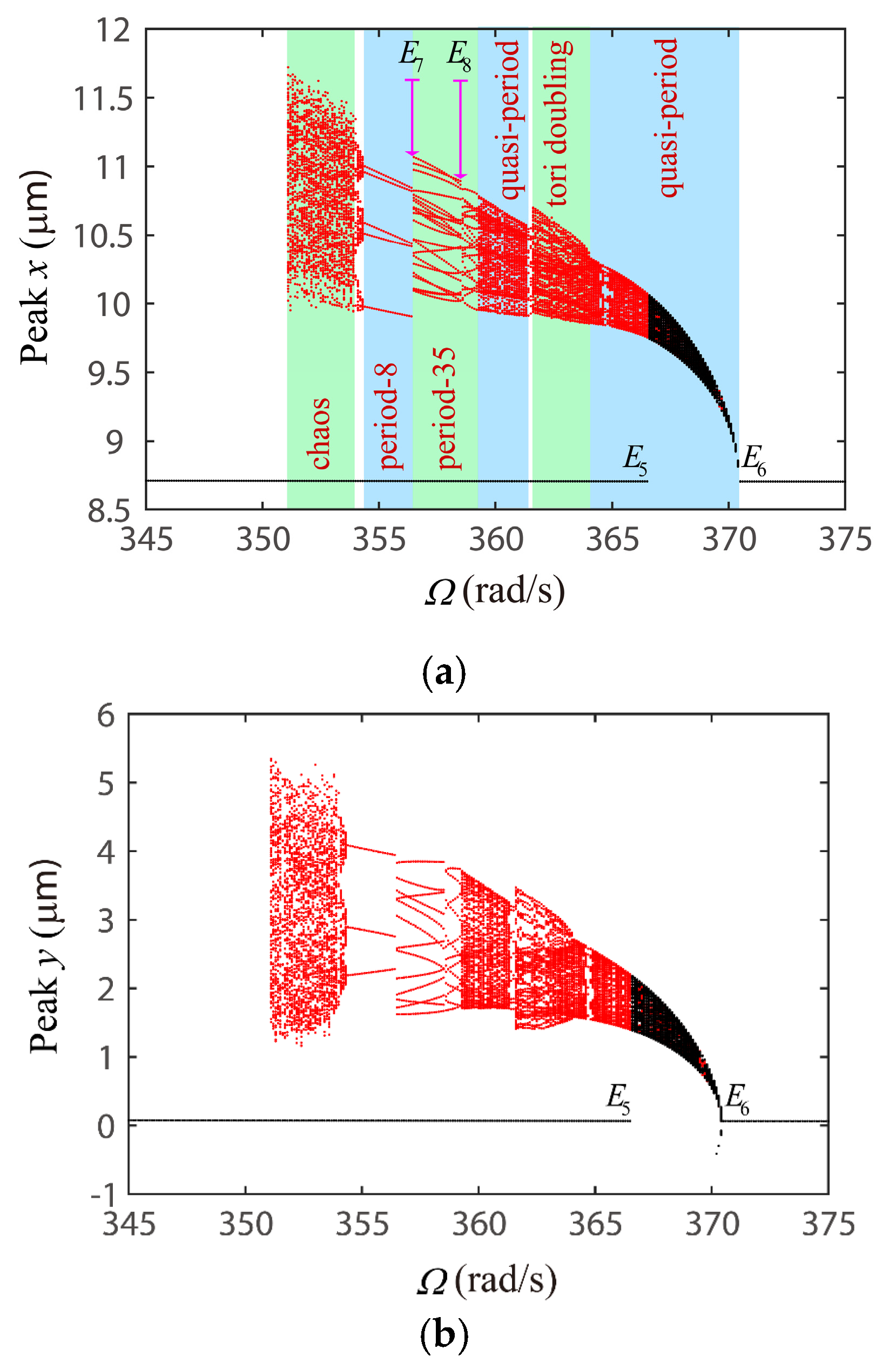
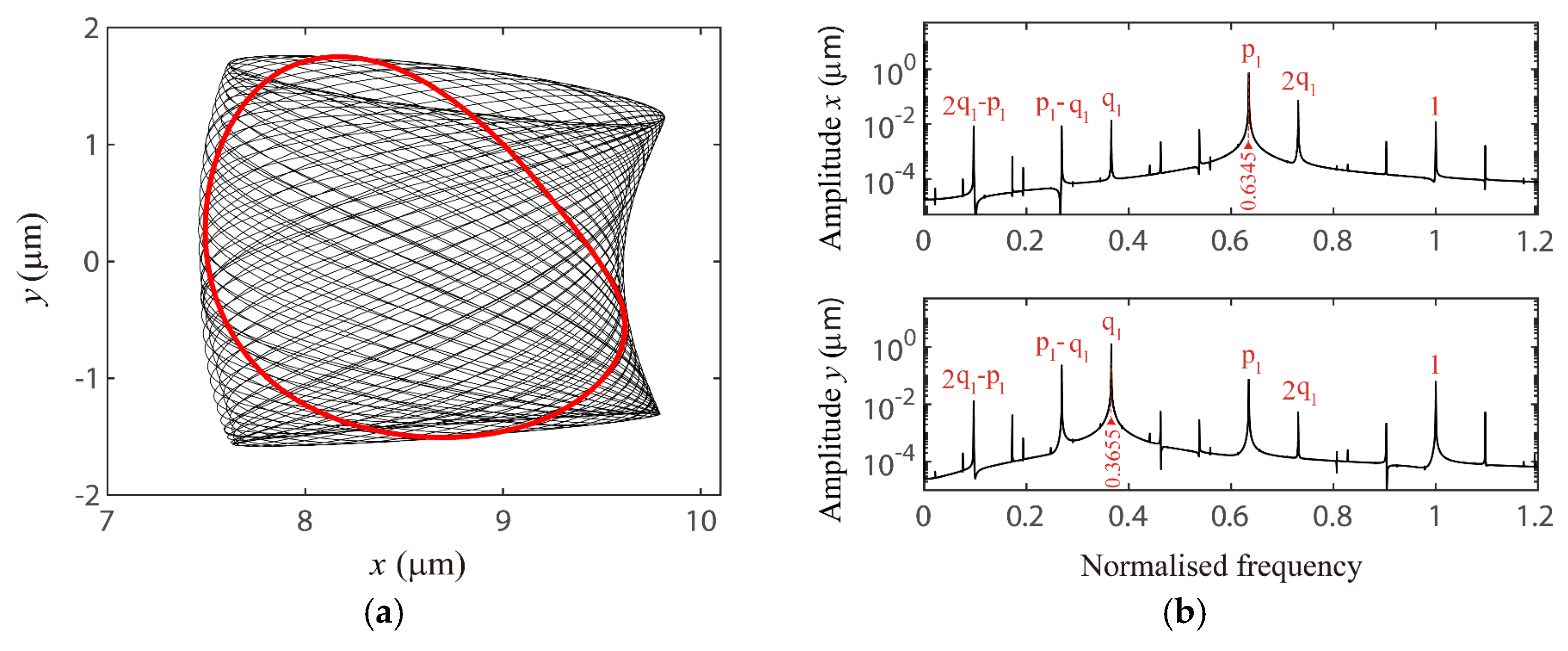
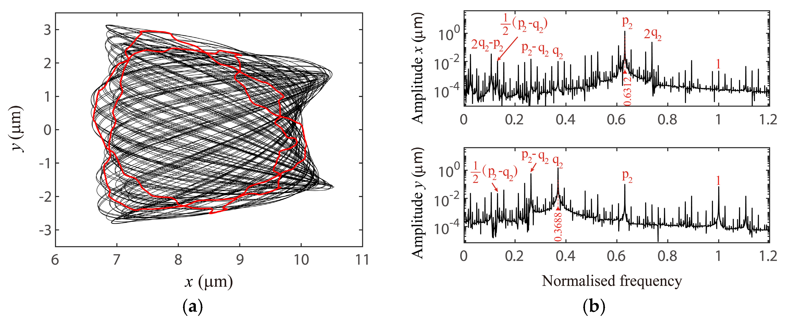
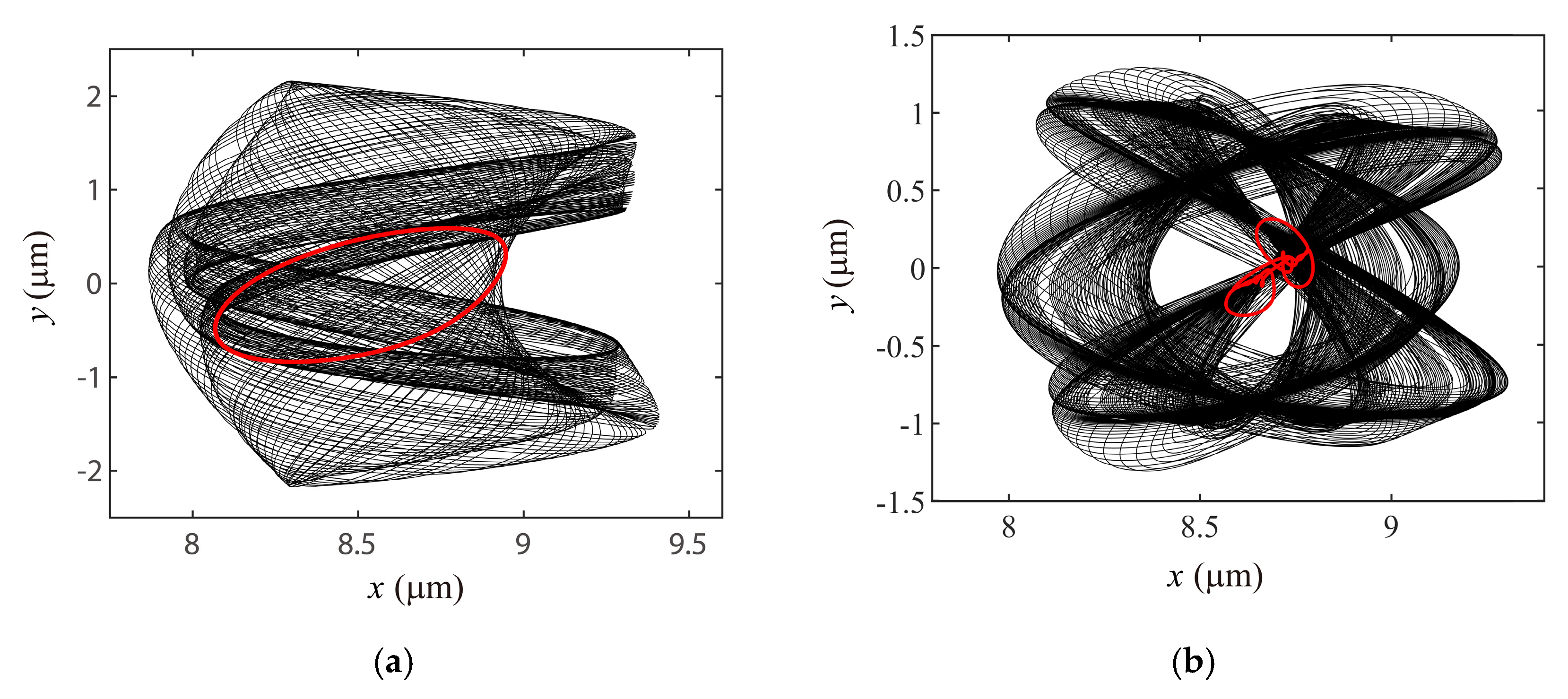
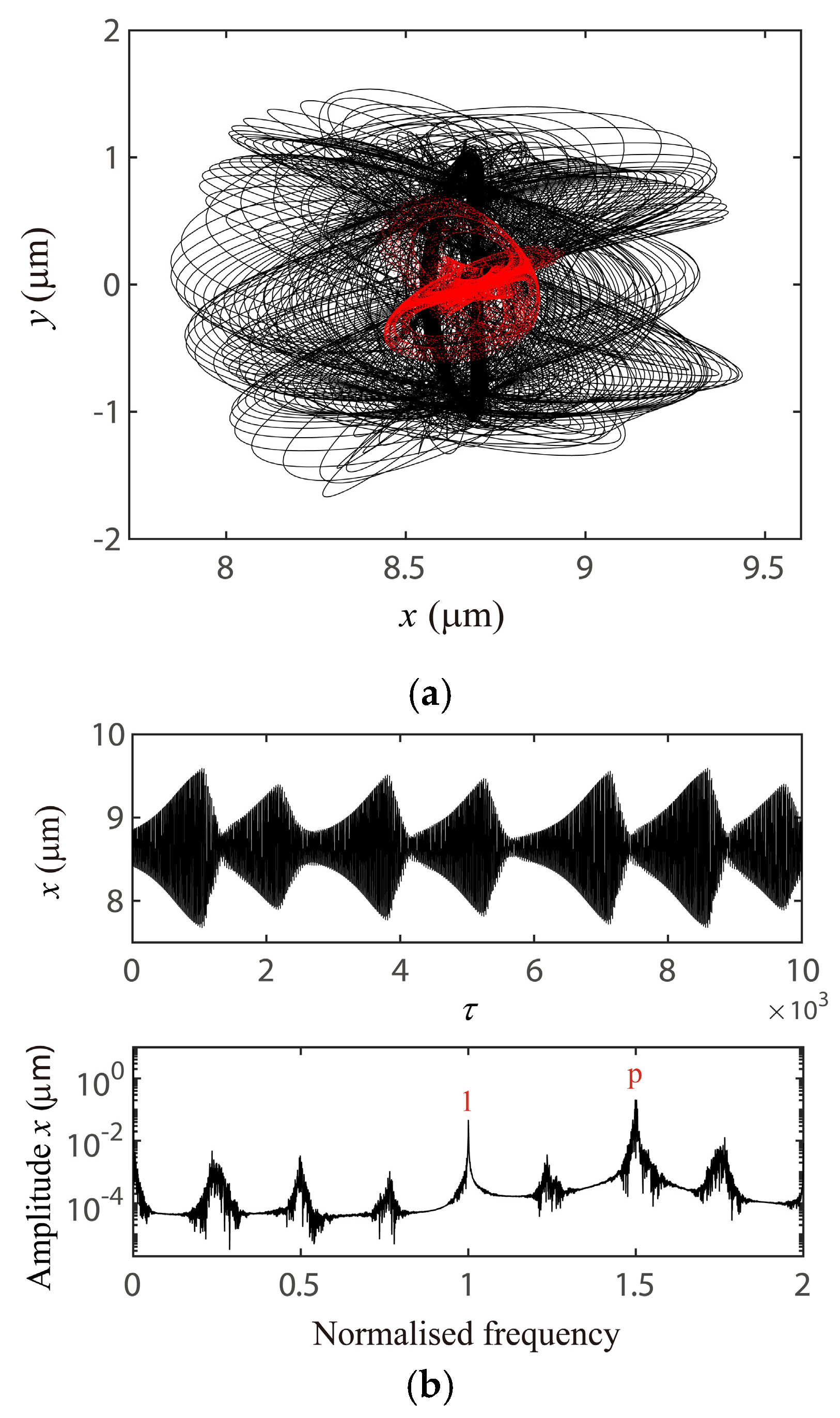
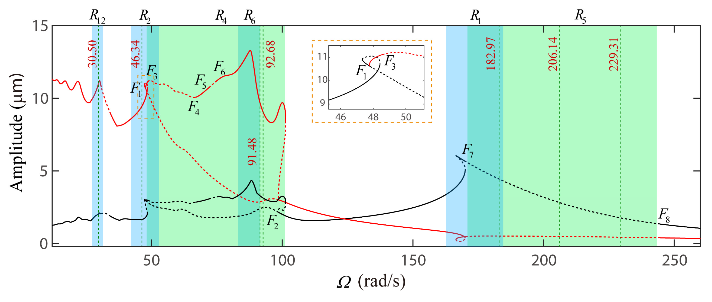
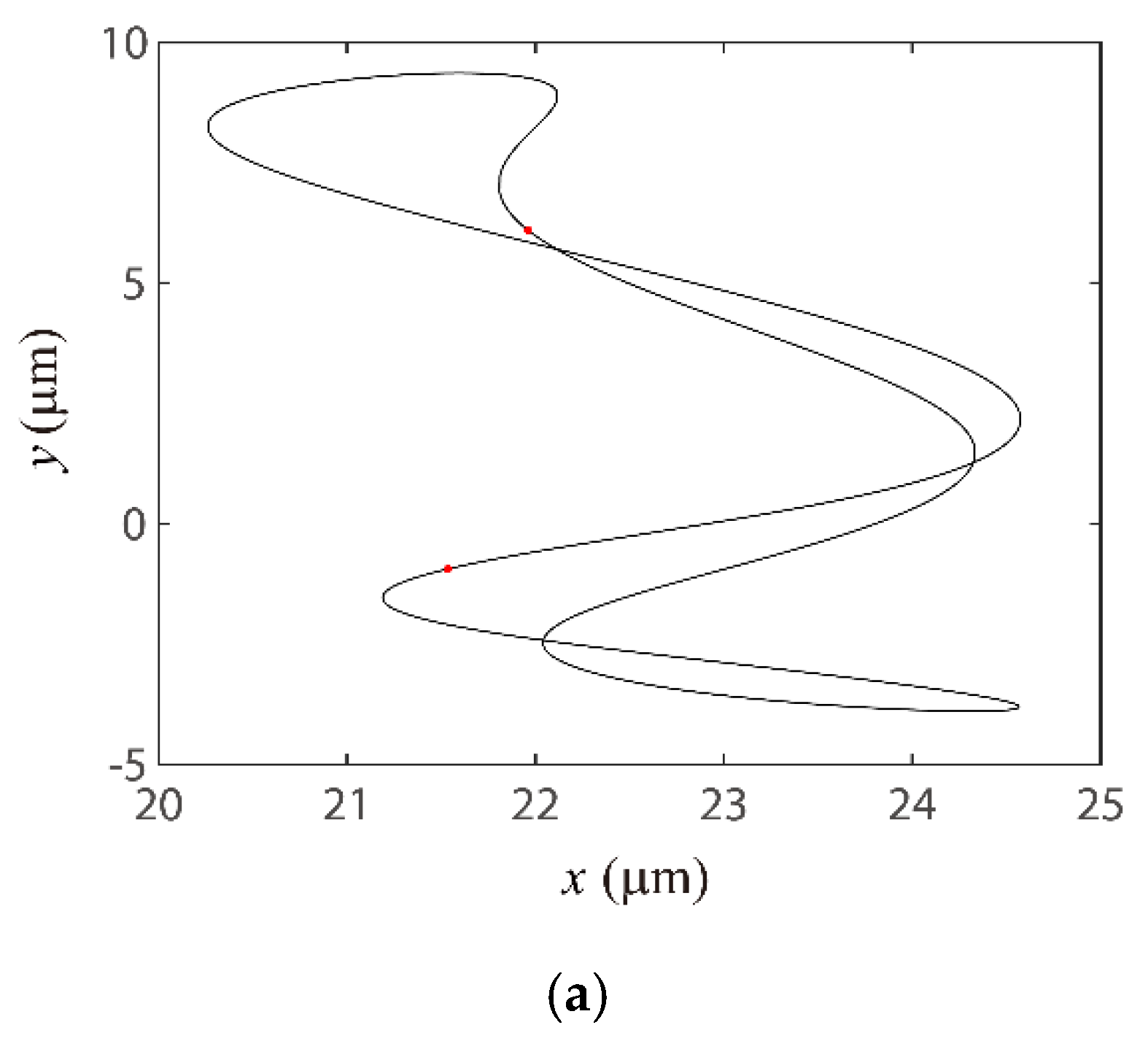
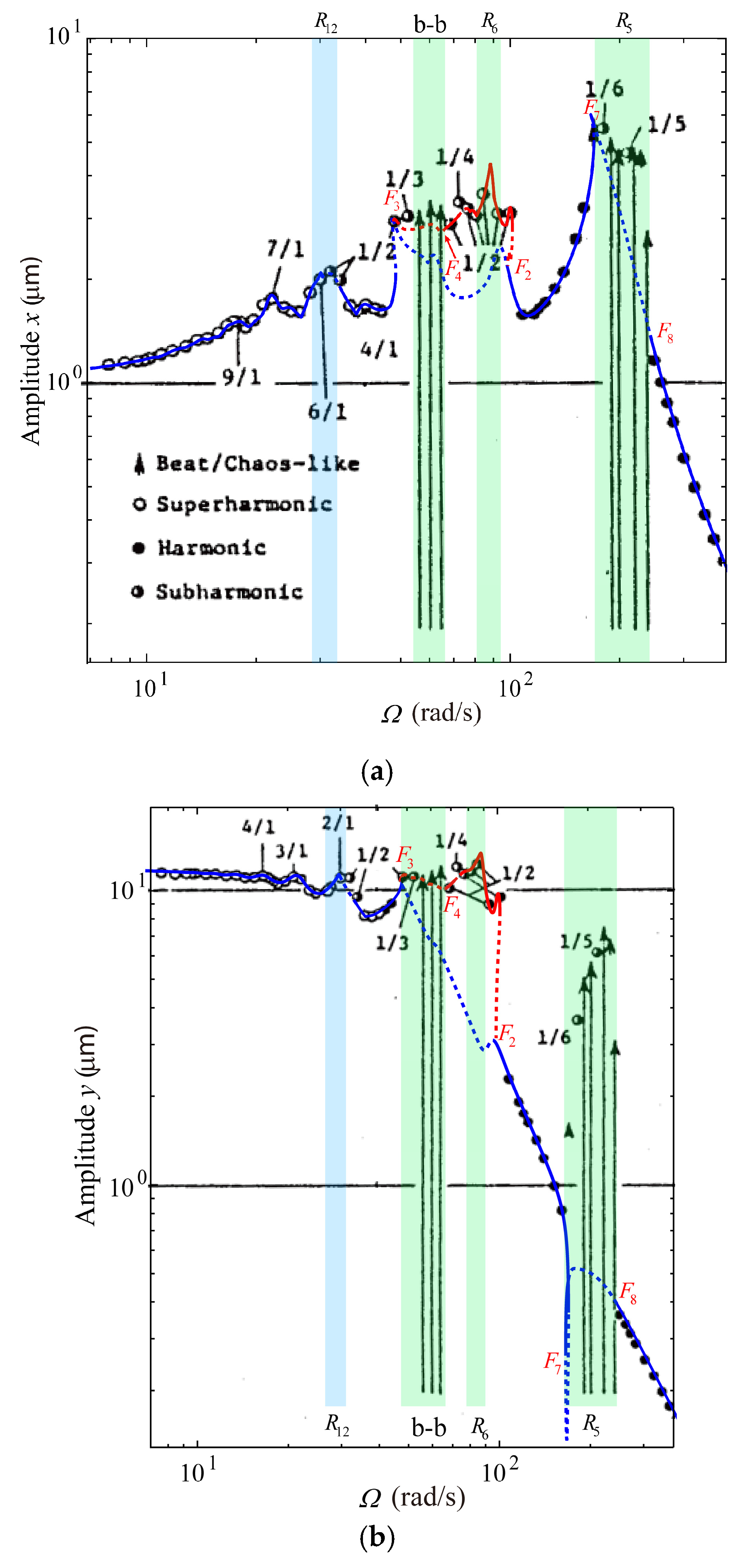
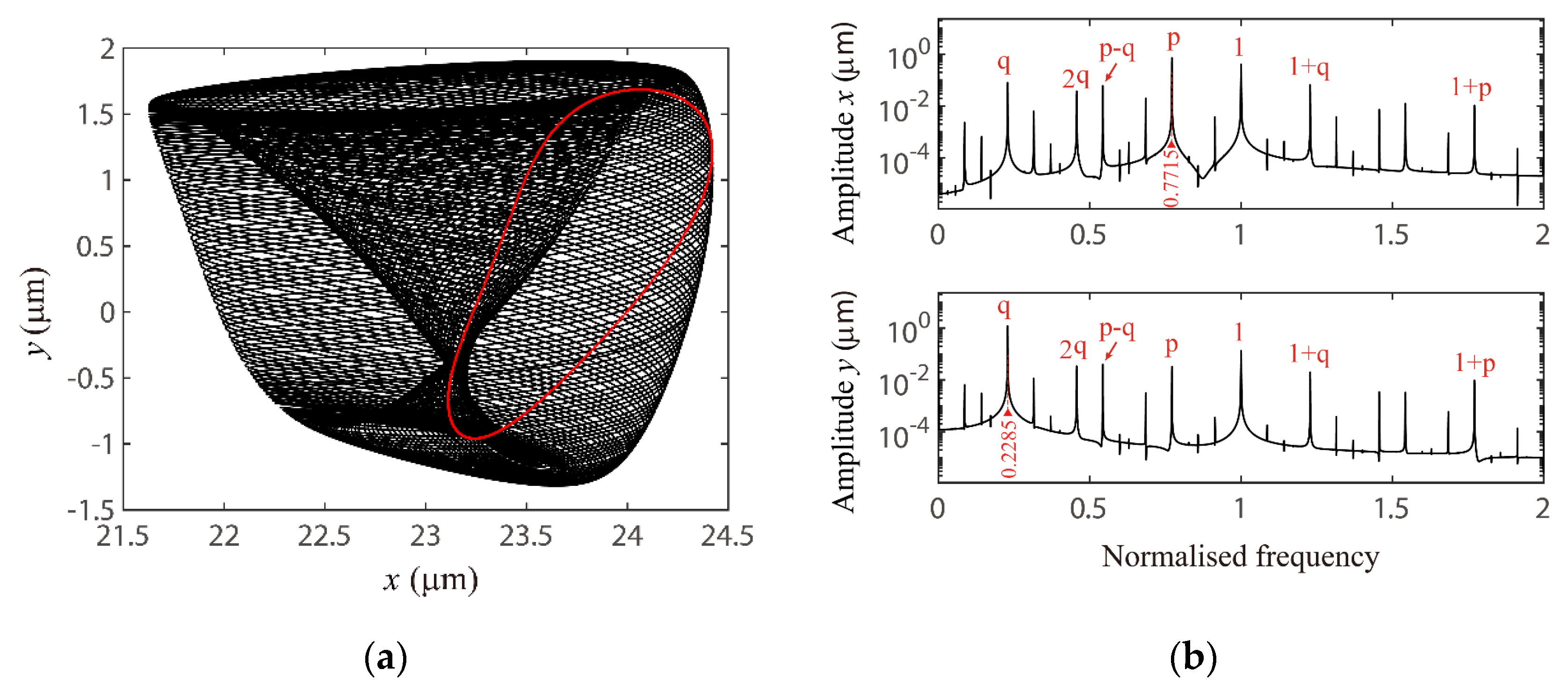
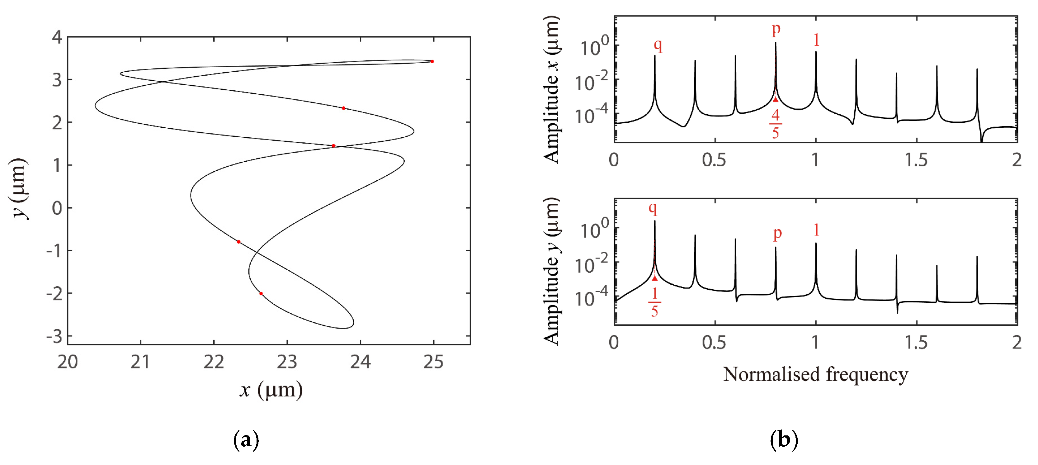
4.2. Global Response Characteristics of VC Resonances around the Bearing Clearance-Free Operations
4.3. Discussion on the Verification of Global VC Parametric Resonances
5. Conclusions
Author Contributions
Funding
Acknowledgments
Conflicts of Interest
References
- Faraday, M. On a peculiar class of acoustical figures; and on certain forms assumed by groups of particles upon vibrating elastic surfaces. Philos. Trans. R. Soc. 1830, 3, 49–51. [Google Scholar]
- Akhmedov, E.K.; Dighe, A.; Lipari, P.; Smirnov, A.Y. Atmospheric neutrinos at Super-Kamiokande and parametric resonance in neutrino oscillations. Nucl. Phys. B 1999, 542, 3–30. [Google Scholar] [CrossRef]
- Jürgen, B.; Serreau, J. Parametric resonance in quantum field theory. Phys. Rev. Lett. 2003, 91, 111601. [Google Scholar]
- Blocki, W. Ship safety in connection with parametric resonance of the roll. Int. Shipbuild. Progr. 1980, 27, 36–53. [Google Scholar] [CrossRef]
- Di Leonardo, R.; Ruocco, G.; Leach, J.; Padgett, M.J.; Wright, A.J.; Girkin, J.M.; Burnham, D.R.; McGloin, D. Parametric resonance of optically trapped aerosols. Phys. Rev. Lett. 2007, 99, 010601. [Google Scholar] [CrossRef] [PubMed]
- Mei, C.C.; Zhou, X. Parametric resonance of a spherical bubble. J. Fluid. Mech. 1991, 229, 29–50. [Google Scholar] [CrossRef]
- Zhang, W.; Baskaran, R.; Turner, K. Tuning the dynamic behavior of parametric resonance in a micromechanical oscillator. Appl. Phys. Lett. 2003, 82, 130–132. [Google Scholar] [CrossRef]
- Rhoads, J.F.; Shaw, S.W.; Turner, K.L.; Moehlis, J.; DeMartini, B.E.; Zhang, W. Generalized parametric resonance in electrostatically actuated microelectromechanical oscillators. J. Sound Vib. 2006, 296, 797–829. [Google Scholar] [CrossRef]
- Sunnersjö, C.S. Varying compliance vibrations of rolling bearings. J. Sound Vib. 1978, 58, 363–373. [Google Scholar] [CrossRef]
- Qaderi, M.S.; Hosseini, S.A.A.; Zamanian, M. Combination Parametric Resonance of Nonlinear Unbalanced Rotating Shafts. ASME J. Comput. Nonlinear Dynam. 2018, 13, 111002. [Google Scholar] [CrossRef]
- Harnoy, A. Bearing Design in Machinery: Engineering Tribology and Lubrication; Marcel D: New York, NY, USA, 2002; pp. 31–33, 431–438. [Google Scholar]
- Harris, T.A. Rolling Bearing Analysis, 4th ed.; John Wiley & Sons: New York, NY, USA, 2001; pp. 968–980. [Google Scholar]
- Lou, J.W.; Luo, T.Y. Analysis Calculation and Application of Rolling Bearing; China Machine Press: Beijing, China, 2009; pp. 79–86. [Google Scholar]
- Fukata, S.; Gad, E.H.; Kondou, T.; Ayabe, T.; Tamura, H. On the radial vibrations of ball bearings (computer simulation). Bull. JSME 1985, 28, 899–904. [Google Scholar] [CrossRef]
- Mevel, B.; Guyader, J.L. Routes to chaos in ball bearings. J. Sound Vib. 1993, 162, 471–487. [Google Scholar] [CrossRef]
- Mevel, B.; Guyader, J.L. Experiments on routes to chaos in ball bearings. J. Sound Vib. 2008, 318, 549–564. [Google Scholar] [CrossRef]
- Tomović, R.A. Simplified mathematical model for the analysis of varying compliance vibrations of a rolling bearing. Appl. Sci. 2020, 10, 670. [Google Scholar] [CrossRef]
- Sankaravelu, A.; Noah, S.T.; Burger, C.P. Bifurcation and chaos in ball bearings. ASME Nonlinear Stoch. Dyn. 1994, AMD-192, 313–325. [Google Scholar]
- Ghafari, S.H.; Abdel-Rahman, E.M.; Golnaraghi, F.; Ismail, F. Vibrations of balanced fault-free ball bearings. J. Sound Vib. 2010, 329, 1332–1347. [Google Scholar] [CrossRef]
- Nayak, R. Contact vibrations. J. Sound Vib. 1972, 22, 297–322. [Google Scholar] [CrossRef]
- Hess, D.; Soom, A. Normal vibrations and friction under harmonic loads: Part 1: Hertzian contact. ASME J. Tribol. 1991, 113, 80–86. [Google Scholar] [CrossRef]
- Zhang, Z.Y.; Chen, Y.S.; Cao, Q.J. Bifurcations and hysteresis of varying compliance vibrations in the primary parametric resonance for a ball bearing. J. Sound Vib. 2015, 350, 171–184. [Google Scholar] [CrossRef]
- Zhang, Z.Y.; Chen, Y.S.; Li, Z.G. Influencing factors of the dynamic hysteresis in varying compliance vibrations of a ball bearing. Sci. China Technol. Sci. 2015, 58, 775–782. [Google Scholar] [CrossRef]
- Jin, Y.; Yang, R.; Hou, L.; Chen, Y.; Zhang, Z. Experiments and numerical results for varying compliance contact resonance in a rigid rotor-ball bearing system. ASME J. Tribol. 2017, 139, 041103. [Google Scholar] [CrossRef]
- Zhang, Z.; Sattel, T.; Tan, A.S.; Rui, X.; Yang, S.; Yang, R.; Ying, Y.; Li, X. Suppression of complex hysteretic resonances in varying compliance vibration of a ball bearing. Shock Vib. 2020, 2020, 8825902. [Google Scholar] [CrossRef]
- Zhang, Z.; Rui, X.; Yang, R.; Chen, Y. Control of period-doubling and chaos in varying compliance resonances for a ball bearing. ASME J. Appl. Mech. 2020, 87, 021005. [Google Scholar] [CrossRef]
- Nayfeh, A.H.; Mook, D.T. Nonlinear Oscillations; John Wiley & Sons: New York, NY, USA, 1995; pp. 20–26. [Google Scholar]
- Tiwari, M.; Gupta, K. Effect of radial internal clearance of a ball bearing on the dynamics of a balanced horizontal rotor. J. Sound Vib. 2002, 38, 723–756. [Google Scholar] [CrossRef]
- Tiwari, M.; Gupta, K.; Prakash, O. Dynamic response of an unbalanced rotor supported on ball bearings. J. Sound Vib. 2000, 238, 757–779. [Google Scholar] [CrossRef]
- Harsha, S.P. Nonlinear dynamic analysis of a high-speed rotor supported by rolling element bearings. J. Sound Vib. 2006, 290, 65–100. [Google Scholar] [CrossRef]
- Upadhyay, S.H.; Haesha, S.P.; Jain, S.C. Analysis of Nonlinear Phenomena in High Speed Ball Bearings due to Radial Clearance and Unbalanced Rotor Effects. J. Vib. Control 2010, 16, 65–88. [Google Scholar] [CrossRef]
- Bai, C.Q.; Xu, Q.Y.; Zhang, X.L. Nonlinear stability of balanced rotor due to effect of ball bearing internal clearance. Appl. Math. Mech. 2006, 27, 175–186. [Google Scholar] [CrossRef]
- Ehrich, F.F. High order subharmonic response of high speed rotors in bearing clearance. ASME J. Vibr. Acoust. 1988, 110, 9–16. [Google Scholar] [CrossRef]
- Yoshida, N.; Takano, T.; Yabuno, H.; Inoue, T.; Ishida, Y. 1/2-Order Subharmonic Resonances in Horizontally Supported Jeffcott Rotor; IDETC/CIE, ASME: Washington, DC, USA, 2011; Paper No. DETC2011-47605. [Google Scholar]
- Bai, C.Q.; Zhang, H.Y.; Xu, Q.Y. Subharmonic resonance of a symmetric ball bearing-rotor system. Int. J. Non-Linear Mech. 2013, 50, 1–10. [Google Scholar] [CrossRef]
- Wu, D.; Han, Q.; Wang, H.; Zhou, Y.; Wei, W.; Wang, H.; Xie, T. Nonlinear dynamic analysis of rotor-bearing-pedestal systems with multiple fit clearances. IEEE Access 2020, 8, 26715–26725. [Google Scholar] [CrossRef]
- Yamamoto, T.A. On the critical speeds of a shaft. Mem. Fac. Eng. Nagoya Univ. 1954, 6, 160–170. [Google Scholar]
- Oswald, F.B.; Zaretsky, E.V.; Poplawski, J.V. Effect of internal clearance on load distribution and life of radially loaded ball and roller bearings. Tribol. T. 2012, 55, 245–265. [Google Scholar] [CrossRef]
- Schaeffler Technologies AG & Co. KG. The Design of Rolling Bearing Mountings: Design Examples Covering Machines, Vehicles and Equipment; Fag Bearing company Ltd.: Schweinfurt, Germany, 2012; Publ. No. WL 00 200/5 EA; pp. 11–15. [Google Scholar]
- Cameron, T.M.; Griffin, J.H. An alternating frequency/time domain method for calculating the steady state response of nonlinear dynamic systems. ASME J. Appl. Mech. 1989, 56, 149–154. [Google Scholar] [CrossRef]
- Kim, Y.B.; Choi, S.K. A multiple harmonic balance method for the internal resonant vibration of a non-linear Jeffcott rotor. J. Sound Vib. 1997, 208, 745–761. [Google Scholar] [CrossRef]
- Guskov, M.; Thouverez, F. Harmonic balance-based approach for quasi-periodic motions and stability analysis. ASME J. Vib. Acoust. 2012, 134, 03100335. [Google Scholar] [CrossRef]
- Chen, Y.; Rui, X.; Zhang, Z.; Shehzad, A. Improved incremental transfer matrix method for nonlinear rotor-bearing system. Acta Mech. Sinica-PRC 2020, 36, 1119–1132. [Google Scholar] [CrossRef]
- Ehrich, F.F. Handbook of Rotordynamics; McGraw-Hill: New York, NY, USA, 1992; pp. 60–116. [Google Scholar]
- Adams, M.L. Rotating Machinery Vibration: From Analysis to Troubleshooting; Taylor & Francis: New York, NY, USA, 2009; pp. 230–235. [Google Scholar]
- Erwin, K. Dynamics of Rotor and Foundation; Springer: Berlin, Germany, 1993; pp. 129–138. [Google Scholar]
- Teschl, G. Ordinary Differential Equations and Dynamical Systems; University of Vienna: Vienna, Austria, 2000; Lecture Notes; pp. 65–76. [Google Scholar]
- Chen, Y.S. Nonlinear Vibrations; High Education Press: Beijing, China, 2002; pp. 218–231. [Google Scholar]
- Li, C.; Qiao, R.; Tang, Q.; Miao, X. Investigation on the vibration and interface state of a thin-walled cylindrical shell with bolted joints considering its bilinear stiffness. Appl. Acoust. 2020, 172, 107580. [Google Scholar] [CrossRef]
- Huang, X.D.; Zeng, Z.G.; Ma, Y.N. The Theory and Methods for Nonlinear Numerical Analysis; Wuhan University Press: Wuhan, China, 2004; pp. 79–170. [Google Scholar]
- Nayfeh, A.H.; Balachandran, B. Applied Nonlinear Dynamics; WILEY-VCH: Weinheim, Germany, 2004; pp. 159–170. [Google Scholar]
- Held, G.A.; Jeffries, C.; Haller, E.E. Observation of chaotic behavior in an Electron-hole plasma in Ge. Phys. Rev. Lett. 1984, 52, 1037–1040. [Google Scholar] [CrossRef]
- Yamamoto, T.A. Response curves at the critical speeds of subharmonic and summed and differential harmonic oscillations. Bull. JSME 1960, 3, 397–403. [Google Scholar] [CrossRef]
- Panda, L.N.; Kar, R.C. Nonlinear dynamics of a pipe conveying pulsating fluid with parametric and internal resonances. Nonlinear Dyn. 2007, 49, 9–30. [Google Scholar] [CrossRef]
- Bamadev, S.; Panda, L.N.; Pohit, G. Combination, principal parametric and internal resonances of an accelerating beam under two frequency parametric excitation. Int. J. Non-Linear Mech. 2016, 78, 35–44. [Google Scholar]
- Fang, B.; Wan, S.; Zhang, J.; Hong, J. Research on the influence of clearance variation on the stiffness fluctuation of ball bearing under different operating conditions. J. Mech. Des. 2020, 143, 023403. [Google Scholar] [CrossRef]
- Yamamoto, T.A.; Saito, A. On the vibrations of summed and differential types under parametric excitation. Mem. Fac. Eng. Nagoya Univ. 1970, 22, 54–123. [Google Scholar]
- Thompson, J.M.T.; Stewart, H.B.; Ueda, Y. Safe, explosive, and dangerous bifurcations in dissipative dynamical systems. Phys. Rev. E. 1994, 49, 1019–1027. [Google Scholar] [CrossRef]
- Zhang, Z.Y. Bifurcation and Hysteresis of Varying Compliance Vibrations of a Ball Bearing-Rotor System. Ph.D. Thesis, Harbin Institute of Technology, Harbin, China, 2015. [Google Scholar]
- Ishida, Y.; Liu, J.; Inoue, T.; Suzuki, A. Vibrations of an asymmetrical shaft with gravity and nonlinear spring characteristics (isolated resonances and internal resonances). ASME J. Vib. Acoust. 2008, 130, 38–45. [Google Scholar] [CrossRef]
- Yabuno, H.; Kashimura, T.; Inoue, T.; Ishida, Y. Nonlinear normal modes and primary resonance of horizontally supported Jeffcott rotor. Nonlinear Dyn. 2011, 66, 377–387. [Google Scholar] [CrossRef]


| Item | Value |
|---|---|
| Contact stiffness Cb (N/m3/2) | 1.334 × 10¹⁰ |
| Ball diameter Db (mm) | 11.9062 |
| Pitch diameter Dh (mm) | 52.0 |
| Number of balls Nb | 8 |
| Equivalent mass m (kg) | 20 |
| Damping factor c (Ns/m) | 200 |
| Radial load W (N) | 196 |
| Ω | 316.3645 | 316.4645 | 316.5645 | 316.6645 |
|---|---|---|---|---|
| λm | 0.021 + 0.987i | 0.019 + 0.987i | 0.018 + 0.988i | 0.017 + 0.988i |
| 0.021 − 0.987i | 0.019 − 0.987i | 0.018 − 0.988i | 0.017 − 0.988i | |
| −0.988 + 0.009i | −0.995 | −1.002 | −1.006 | |
| −0.988 − 0.009i | −0.980 | −0.974 | −0.969 |
| Ω | 341.7310 | 341.7316 | 341.7316 | 341.7315 |
|---|---|---|---|---|
| λm | −0.536 + 0.817i | −0.535 + 0.818i | −0.535 + 0.818i | −0.535 + 0.818i |
| −0.536 − 0.817i | −0.535 − 0.818i | −0.535 − 0.818i | −0.535 − 0.818i | |
| 0.987 | 0.998 | 1.001 | 1.002 | |
| 0.968 | 0.957 | 0.954 | 0.953 |
| Ω | 406.9645 | 407.0645 | 407.1645 | 407.2645 |
|---|---|---|---|---|
| λm | −0.018 + 1.031i | −0.019 + 1.006i | −0.019 + 0.971i | −0.066 + 0.923i |
| −0.018 − 1.031i | −0.019 − 1.006i | −0.019 − 0.971i | −0.066 − 0.923i | |
| −0.014 + 0.831i | −0.016 + 0.851i | −0.017 + 0.883i | 0.027 + 0.925i | |
| −0.014 − 0.831i | −0.016 − 0.851i | −0.017 − 0.883i | 0.027 − 0.925i |
| Ω | 353 | 355 | 357 | 363 | 368 |
|---|---|---|---|---|---|
| ωx0 (rad/s) | 1767.54 | 1775.00 | 1795.20 | 1833.00 | 1867.97 |
| ωy0 (rad/s) | 1056.46 | 1065.00 | 1060.80 | 1071.00 | 1076.03 |
| Item | Value |
|---|---|
| Contact stiffness Cb (N/m3/2) | 1.334 × 10¹⁰ |
| Ball diameter Db (mm) | 11.9062 |
| Pitch diameter Dh (mm) | 52.0 |
| Number of balls Nb | 8 |
| Bearing clearance δ0 (μm) | 20 |
| Equivalent mass m (kg) | 16 |
| Damping factor c (Ns/m) | 2940 |
| Radial load W (N) | 58.8 |
Publisher’s Note: MDPI stays neutral with regard to jurisdictional claims in published maps and institutional affiliations. |
© 2020 by the authors. Licensee MDPI, Basel, Switzerland. This article is an open access article distributed under the terms and conditions of the Creative Commons Attribution (CC BY) license (http://creativecommons.org/licenses/by/4.0/).
Share and Cite
Zhang, Z.; Sattel, T.; Zhu, Y.; Li, X.; Dong, Y.; Rui, X. Mechanism and Characteristics of Global Varying Compliance Parametric Resonances in a Ball Bearing. Appl. Sci. 2020, 10, 7849. https://doi.org/10.3390/app10217849
Zhang Z, Sattel T, Zhu Y, Li X, Dong Y, Rui X. Mechanism and Characteristics of Global Varying Compliance Parametric Resonances in a Ball Bearing. Applied Sciences. 2020; 10(21):7849. https://doi.org/10.3390/app10217849
Chicago/Turabian StyleZhang, Zhiyong, Thomas Sattel, Yujie Zhu, Xuan Li, Yawei Dong, and Xiaoting Rui. 2020. "Mechanism and Characteristics of Global Varying Compliance Parametric Resonances in a Ball Bearing" Applied Sciences 10, no. 21: 7849. https://doi.org/10.3390/app10217849
APA StyleZhang, Z., Sattel, T., Zhu, Y., Li, X., Dong, Y., & Rui, X. (2020). Mechanism and Characteristics of Global Varying Compliance Parametric Resonances in a Ball Bearing. Applied Sciences, 10(21), 7849. https://doi.org/10.3390/app10217849