1. Introduction
Some of the requirements that are placed on autonomous mobile robotic systems include real-world environments navigation and recognition and identification of objects of interest with which the robotic system have to interact. Computer vision allows machines to obtain a large amount of information from the environment that has a major impact on their behavior. In the surrounding environment there are often numerous different static objects (walls, columns, doors, and production machines) but also moving objects (people, cars, and handling trucks).
Objects that are used to refine navigation, landmarks, can be artificial (usually added by a human) and natural (which naturally occur in the environment) [
1,
2].
Robotic systems have to work in a real environment and must be able to recognize, for example, people [
3], cars [
4], product parameters for the purpose of quality control, or objects which are to be handled.
The use of QR (Quick Response) codes (two-dimensional matrix codes) in interaction with robots can be seen in the following areas:
in the field of navigation as artificial landmarks-analogies of traffic signs that control the movement of the robot in a given area (no entry, driving direction, alternate route, and permitted hours of operation) or as an information board providing context specific information or instructions (such as identification of floor, room, pallets, and working place)
in the area of object identification, 2D codes are often used to mark products and goods and thus their recognition will provide information about the type of goods (warehouses), the destination of the shipment (sorting lines) or control and tracking during track-and-trace.
QR Codes
QR Codes are classified among 2D matrix codes (similar to Data Matrix codes). QR Codes (Model 1 and Model 2) are squared-shaped 2D matrices of dark and light squares—so called modules. Each module represents the binary 1 or 0. Each QR Code has fixed parts (such as Finder Patterns and Timing Patterns) that are common to each QR Code and variable parts that differ according to the data that is encoded by a QR Code. Finder Patterns, which are located in the three corners of a QR Code, are important for determining the position and rotation of the QR Code. The size of the QR code is determined by the number of modules and can vary from 21 × 21 modules (Version 1) to 177 × 177 (Version 40). Each higher version number comprises four additional modules per side. In the
Figure 1 we can see a sample of version 1 QR Code.
QR Code has error correction capability to restore data if the code is partially damaged. Four error correction levels are available (L–Low, M–Medium, Q–Quartile, and H–High). The error correction level determines how much of the QR Code can be corrupted to keep the data still recoverable (L–7%, M–15%, Q–25%, and H–30%) [
5]. The QR Code error correction feature is implemented by adding a Reed–Solomon Code to the original data. The higher the error correction level is the less storage capacity is available for data.
Each QR Code symbol version has the maximum data capacity according to the amount of data, character type and the error correction level. The data capacity ranges from 10 alphanumeric (or 17 numeric) characters for the smallest QR Code up to 1852 alphanumeric (or 3057 numeric) characters for the largest QR Code at highest error correction level [
5]. QR Codes support four encoding modes—numeric, alphanumeric, Kanji and binary—to store data efficiently.
QR Code was designed in 1994, in Japan for automotive industry, but currently has a much wider use. QR codes are used to mark a variety of objects (goods, posters, monuments, locations, and business cards) and allow to attach additional information to them, often in the form of a URL to a web page. QR Code is an ISO standard (ISO/IEC 18004:2015) and is freely available without license fees.
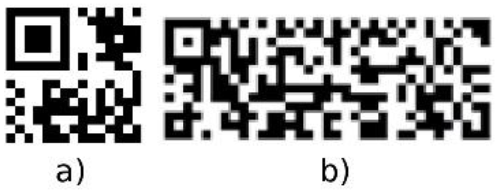
In addition to a traditional QR Code Model 1 and 2, there are also variants such as a Micro QR Code (a smaller version of the QR Code standard for applications where a symbol size is limited) or an iQR Code (which can hold a greater amount of information than a traditional QR Code and it supports also rectangular shapes) (
Figure 2).
2. Related Work
Prior published approaches for recognizing QR Codes in images can be divided into Finder Pattern based location methods [
6,
7,
8,
9,
10,
11,
12] and QR Code region based location methods [
13,
14,
15,
16,
17,
18]. The first group locates a QR Code based on the location of its typical Finder Patterns that are present in its three corners. The second group locates the area of a QR code in the image based on its irregular checkerboard-like structure (a QR Code consists of many small light and dark squares which alternate irregularly and are relatively close to each other).
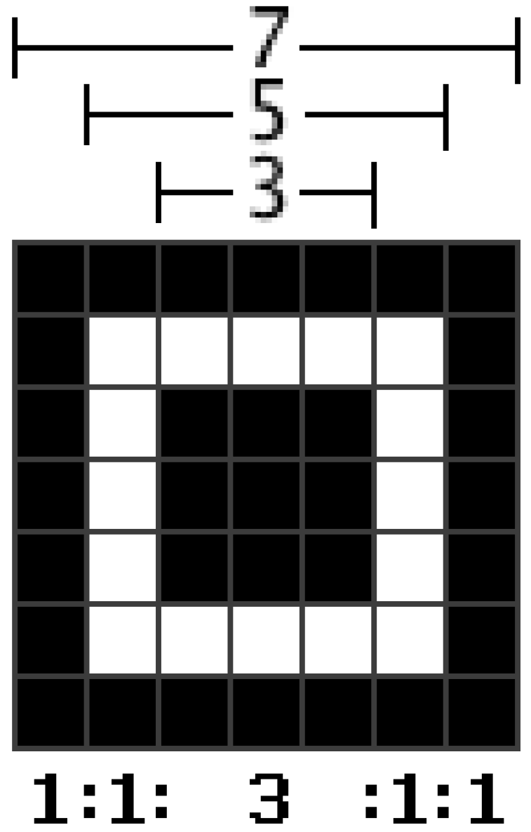
A shape of the Finder Pattern (
Figure 3) was deliberately chosen by the authors of the QR Code, because “it was the pattern least likely to appear on various business forms and the like” [
6]. They found out that black and white areas that alternate in a 1:1:3:1:1 ratio are the least common on printed materials.
In [
7] (Lin and Fuh) all points matching the 1:1:3:1:1 ratio, horizontally and vertically, are collected. Collected points belonging to one Finder Pattern are merged. Inappropriate points are filtered out according to the angle between three of them.
In [
8] (Li et al.) minimal containing region is established analyzing five runs in labeled connected components, which are compacted using run-length coding. Second, coordinates of central Finder Pattern in a QR Code are calculated by using run-length coding utilizing modified Knuth–Morris–Pratt algorithm.
In [
9] (Belussi and Hirata) two-stage detection approach is proposed. In the first stage Finder Pattern (located at three corners of a QR Code) is detected using a cascaded classifier trained according to the rapid object detection method (Viola–Jones framework). In the second stage geometrical restrictions among detected components are verified to decide whether subsets of three of them correspond to a QR Code or not.
In [
10] (Bodnár and Nyúl) Finder Pattern candidate localization is based on the cascade of boosted weak classifiers using Haar-like features, while the decision on a Finder Pattern candidate to be kept or dropped is decided by a geometrical constraint on distances and angles with respect to other probable Finder Patterns. In addition to Haar-like features, local binary patterns (LBP), and histogram of oriented gradients (HOG) based classifiers are used and trained to Finder Patterns and whole code areas as well.
In [
11] (Tribak and Zaz) successive horizontal and vertical scans are launched to obtain segments whose structure complies with the ratio 1:1:3:1:1. The intersection between horizontal and vertical segments presents the central pixel of the extracted pattern. All the extracted patterns are transmitted to a filtering process based on principal components analysis, which is used as a pattern feature.
In [
12] (Tribak and Zaz) seven Hu invariant moments are applied to the Finder Pattern candidates obtained by initial scanning of an image and using Euclidean metrics they are compared with Hu moments of the samples. If the similarity is less than experimentally determined threshold, then the candidate is accepted.
In [
13] (Sun et al.) authors introduce algorithm, which aims to locate a QR Code area by four corners detection of 2D barcode. They combine the Canny edge detector with external contours finding algorithm.
In [
14] (Ciążyński and Fabijańska) they use histogram correlation between a reference image of a QR code and an input image divided into a block of size 30 × 30. Then candidate blocks are joined into regions and morphological erosion and dilation is applied to remove small regions.
In [
15] (Gaur and Tiwari) they propose approach which uses Canny edge detection followed by morphological dilation and erosion to connect broken edges in a QR Code into a bigger connected component. They expect that the QR Code is the biggest connected component in the image.
In [
16,
17] (Szentandrási et al.) they exploit the property of 2D barcodes of having regular distribution of edge gradients. They split a high-resolution image into tiles and for each tile they construct HOG (histogram of oriented gradients) from the orientations of edge points. Then they select two dominant peeks in the histogram, which are apart roughly 90°. For each tile, a feature vector is computed, which contains a normalized histogram, angles of two main gradient directions, a number of edge pixels and an estimation of probability score of a chessboard-like structure.
In [
18] (Sörös and Flörkemeier) areas with high concentration of edge structures as well as areas with high concentration of corner structures are combined to get QR Code regions.
3. The Proposed Method
Our method is primarily based on searching for Finder Patterns and utilizes their characteristic feature—1:1:3:1:1 black and white point ratio in any scanning direction. The basic steps are indicated in the flowchart in
Figure 4.
Before searching for a QR Code, the original image (maybe colored) is converted to a gray scale image using Equation (1), because the color information does not bear any significant additional information that might help in QR Code recognition.
where
I stands for gray level and
R,
G,
B for red, green, and blue color intensities of individual pixels in the RGB model, respetively. This RGB to gray scale conversion is integer approximation of widely used luminance calculation as defined in recommendation ITU-R BT.601-7:
Next, the gray scaled image is converted to a binary image using modified adaptive thresholding (with the size of window 35—the window size we choose to be at least five times the size of expected size of QRC module) [
19]. We expect that black points, which belong to QRC, will become foreground points.
We use the modification of the well-known adaptive thresholding technique (Equation (3)), which calculates individual threshold for every point in the image. This threshold is calculated using average intensity of points under a sliding window. To speed up the thresholding we pre-calculate the integral sum image and we also use the global threshold value (points with intensity above 180 we always consider as background points). Adaptive thresholding can successfully threshold also uneven illuminated images.
where
I is gray scale (input) image,
B is binary (output) image,
T is threshold value (individual for each pixel at coordinates
x,
y), and
m is average of pixel intensities under sliding window of the size 35 × 35 pixels.
In order to improve adaptive thresholding results, some of the image pre-processing techniques, such as histogram equalization, contrast stretching or deblurring, are worth to consider.
3.1. Searching for Finder Patterns
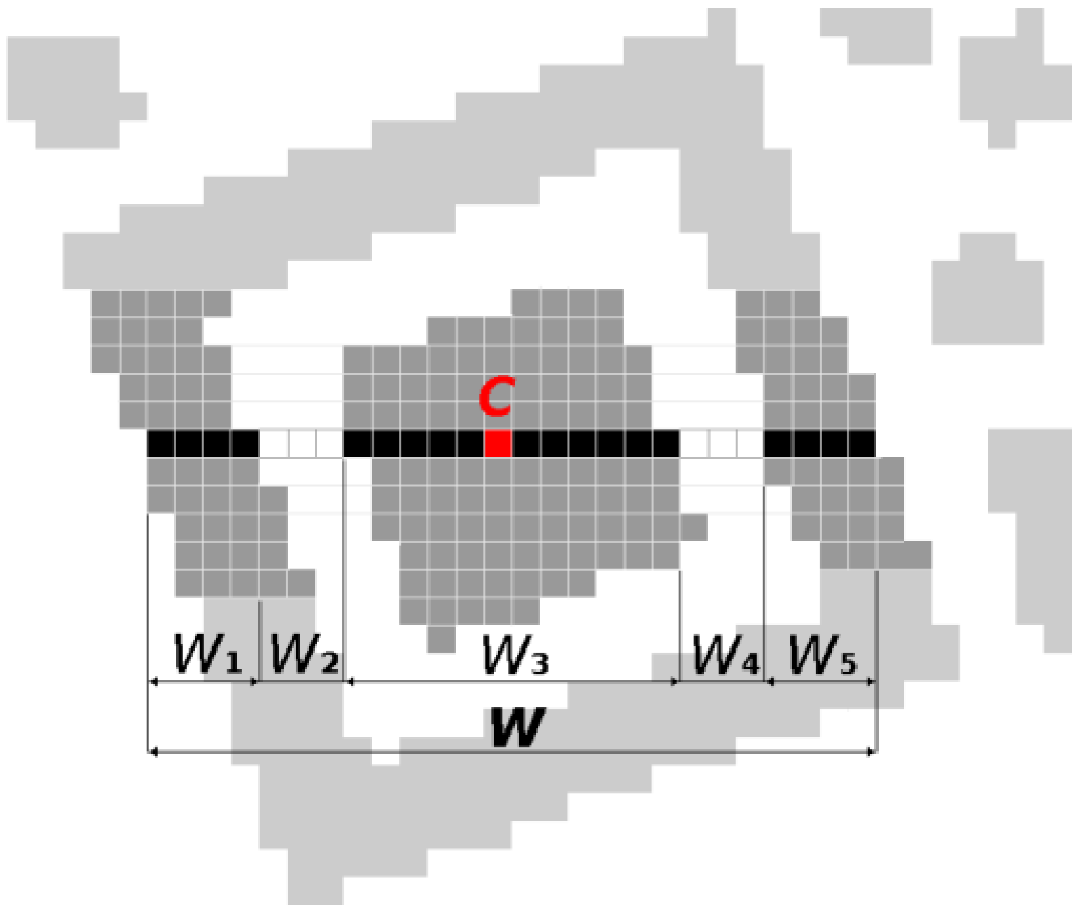
First, the binary image is scanned from top to bottom and from left to right, and we look for successive sequences of black and white points in a row matching the ratios 1:1:3:1:1 (
W1:
W2:
W3:
W4:
W5 where
W1,
W3,
W5 indicates the number of consecutive black points which are alternated by
W2,
W4 white points) with small tolerance (tolerance is necessary due to imperfect thresholding and noise in the Finder Pattern area, black and white points in a line do not alternate in ideal ratios 1:1:3:1:1):
For each match in a row coordinates of Centroid (
C) and Width (
W =
W1 +
W2 +
W3 +
W4 +
W5) of the sequence (of black and white points) are stored in a list of Finder Pattern candidates (
Figure 5).
Then, Finder Pattern candidates (from the list of candidates) that satisfy the following criteria are grouped:
their centroids C are at most 3/7W points vertically and at most 3 points horizontally away from each other,
their widths W does not differ by more than 2 points.
We expect, that the Finder Pattern candidates in one group belong to the same Finder Pattern and therefore we set the new centroid
C and width
W of the group as average of
x,
y coordinates and widths of the nearby Finder Pattern candidates (
Figure 6a).
After grouping the Finder Patterns, it must be verified whether there are sequences of black and white points also in the vertical direction, which alternate in the ratio 1:1:3:1:1 (
Figure 6b). A bounding box around the Finder Pattern candidate, in which vertical sequences are looked for, is defined as
where
C (
Cx,
Cy) is a centroid and
W is width of the Finder Pattern candidate. We work with a slightly larger bounding box in case the Finder Pattern is stretched vertically. Candidates, where no vertical match is found or where the ratio
H/
W < 0.7, are rejected. For candidates, where a vertical match is found, the
y coordinate of centroid
C (
Cy) is updated as an average of
y coordinates of centers of the vertical sequences.
3.2. Verification of Finder Patterns
Each Finder Pattern consists of a central black square with the side of 3 units (
R1), surrounded by a white frame with the width of 1 unit (
R2), surrounded by a black frame with the width of 1 unit (
R3). In
Figure 7 there are colored regions
R1,
R2 and
R3 in red, blue, and green, respectively. For each Finder Pattern candidate Flood Fill algorithm is applied, starting from the centroid
C (which lies in the region
R1) and continuing through white frame (region
R2) to black frame (region
R3). As continuous black and white regions are filled, following region descriptors are incrementally computed:
area (A = M00)
centroid (Cx = M10/M00, Cy = M01/M00), where M00, M10, M00 are raw image moments
bounding box (Top, Left, Right, Bottom)
The Finder Pattern candidate, which does not meet all of the following conditions, is rejected.
Area(R1) < Area(R2) < Area(R3) and
1.1 < Area(R2)/Area(R1) < 3.4 and
1.8 < Area(R3)/Area(R1) < 3.9
0.7 < AspectRatio(R2) < 1.5 and
0.7< AspectRatio(R3) < 1.5
|Centroid(R1), Centroid(R2)| < 3.7 and
|Centroid(R1), Centroid(R3)| < 4.2
Note: the criteria were set to be invariant to the rotation of the Finder Pattern, and the acceptance ranges were determined experimentally. In an ideal undistorted Finder Pattern, the criteria are met as follows:
Area(R2)/Area(R1) = 16/9 = 1.8 and Area(R3)/Area(R1) = 24/9 = 2.7
AspectRatio(R1) = 1 and AspectRatio(R2) = 1 and AspectRatio(R3) = 1
Centroid(R1) = Centroid(R2) = Centroid(R3)
In real environments there can be damaged Finder Patterns. The inner black region
R1 can be joined with the outer black region
R3 (
Figure 8a) or the outer black region can be interrupted or incomplete (
Figure 8b). In the first case the bounding box of the region
R2 is completely contained by bounding box of the region
R1 and in the second case is bounding box of the region
R3 contained in bounding box of the region
R2. These cases are handled individually. If the first case is detected, then the region
R1 is proportionally divided into
R1 and
R3 and if the second case is detected then the region
R2 is instantiated using the region
R1 and
R3.
The Centroid (
C) and Module Width (
MW) of the Finder Pattern candidate are updated using the region descriptors as follows:
3.3. Grouping of Finder Patterns
3.3.1. Grouping Triplets of Finder Patterns
In the previous steps, Finder Patterns in the image were identified and now such triplets (from the list of all Finder Patterns) must be selected, which can represent 3 corners of a QR Code. Matrix of the distances between the centroid of all Finder Patterns is build and all 3-element combinations of all Finder Patterns are examined. For each triplet it is checked whether it is possible to construct a right-angled triangle from it so that the following conditions are met:
the size of each triangle side must be in predefined range
the difference in sizes of two legs must be less than 21
the difference in size of the real and theoretical hypotenuse must be less than 12
In this way, a list of QR Code candidates (defined by a triplet FP
1, FP
2, FP
3) is built. However, such a candidate for a QR Code is selected only on the basis of the mutual position of the 3 FP candidates. As is shown in
Figure 9 not all QR Code candidates are valid (dotted red FP
3′-FP
3″-FP
2″ is false positive). These false positive QR Code candidates will be eliminated in the next steps.
Finally, Bottom-Left and Top-Right Finder Pattern from the triplet (FP1, FP2, FP3) is determined by using formula:
If (FP3.x − FP2.x)(FP1.y − FP2.y) − (FP3.y − FP2.y)(FP1.x − FP2.x) < 0 then Bottom-Left is FP3 and Top-Right is FP1 else vice versa.
3.3.2. Grouping Pairs of Finder Patterns
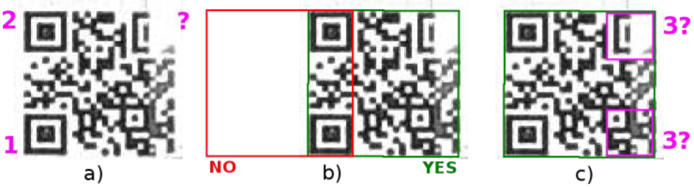
If any QR Code has one of the 3 Finder Patterns significantly damaged, then this Finder Pattern might not be identified and there remains two Finder Patterns in the Finder Patterns list, that were not selected (as the vertices of a right-angled triangle) in the previous step (
Figure 10a). The goal of this step is to identify these pairs and determine the position of the third missing Finder Pattern. A square shape of the QR Code is assumed.
All two element combinations of remaining Finder Patterns, whose distance is in a predefined interval, are evaluated. A pair of Finder Patterns can represent Finder Patterns that are adjacent corners of a QR Code square (
Figure 10a) or are in the opposite corners. If they are adjacent corners, then there are two possible positions of the QR Code (in
Figure 10b depicted as a red square and green square). If they are opposite corners, then there are other two possible positions of the QR Code.
All four possible positions of the potential QR Code are evaluated against the following criteria:
Is there a Quiet Zone around the bounding square at least 1 MW wide?
Is there a density of white points inside bounding square in interval (0.4; 0.65)?
Is there a density of edge points inside bounding square in interval (0.4; 0.6)?
Density of edge points is computed as the ratio of the number of edge points to area*2/MW.
Region of a QR Code is expected to have relative balanced density of white and black points and relative balanced ratio of edges to area.
A square region that meets all the above conditions is considered a candidate for a QR Code. There are two possible corners in the QR Code bounding square where 3rd Finder Pattern can be located (
Figure 10c). For both possible corners Finder Pattern match score is computed and one with better score is selected (in other words question, “In which corner is the structure that more closely resembles the ideal Finder Pattern?” must be answered). Match score is computed as
where
MS is match score (lower is better),
OS is overall pattern match score,
BS is black module match score and
WS is white module match score.
BS stores matches only for expected black points and
WS stores matches only for expected white points between the mask and the image.
BS and
WS was introduced to handle situations when over the area of Finder Pattern is placed black or white spot, which would cause a low match score if only a simple pattern matching technique were used.
The match score is computed for several Finder Pattern mask positions by moving the mask in a spiral from its initial position up to a radius of MW with a step of MW/2 (for the case of small geometric deformations of the QR Code).
3.4. Verification of Quiet Zone
According to ISO standard a Quiet Zone is defined as “a region 4X wide which shall be free of all other markings, surrounding the symbol on all four sides”. So, it must be checked if there are only white points in the image in the rectangular areas wide 1
MW which is parallel to line segments defined by FP
1–FP
2 and FP
2–FP
3 (
Figure 11). For fast scanning of the rectangle points Bresenham’s line algorithm is utilized [
20].
QR Code candidates which do not have quiet zones around are rejected. Rejected are also QR Code candidates whose outer bounding box (larger) contains outer bounding box (smaller) of another QR Code candidate.
3.5. QR Code Bounding Box
Centroids of the 3 Finder Patterns (which represent the QR Code candidate) are the vertices of the triangle FP
1–FP
2–FP
3. This inner triangle must be expanded to outer triangle P
1–P
2–P
3, where the arms of the triangle pass through boundary modules of the QR Code (
Figure 12). For instance, the shift of FP
3 to P
3 may be expressed as
where
MW is module width (Equation (6))
3.6. Perspective Distortion
For perspective undistorted QR Codes (only shifted, scaled, rotated, or sheared) it is sufficient to have only 3 points to set-up the affine transformation from a square to destination parallelogram. However, for perspective (projective) distorted QR Codes 4 points are required to set-up perspective transformation from a square to destination quadrilateral [
21].
Some authors (for example [
7,
22]) search for Alignment Pattern to obtain 4th point. However, version 1 QR Codes does not have Alignment Pattern, so we have decided not to rely on Alignment Patterns.
Instead of that we use an iterative approach to find the opposite sides to P2–P1 and P2–P3, which aligns to QR Code borders.
We start from initial estimate of P
4 as an intersection of the line L
1 and L
3, where L
1 is parallel to P
2–P
3 and L
3 is parallel to P
2–P
1 (
Figure 13a).
We count the number of pixels which are common to the line L
3 and the QR Code for each third of the line L
3 (
Figure 13a).
We shift the line L
3 by width of one module away from the QR Code and again we count the number of pixels which are common to the shifted line L
3′ and the QR Code. The module width is estimated as
MW (from Equation (6)) (
Figure 13b).
We compare overlaps of the line L3 from the step 2 and 3, and
If L3 was whole in the QR Code and the shifted L3′ is out of the QR Code, then initial estimation of P4 is good and we end.
If L3 was whole in the QR Code and 3rd third of the shifted L3′ is again in the QR Code, then we continue by step 5.
If 3rd third of L3 was in quiet zone and 2nd and 3rd third of the shifted L3′ is in the quiet zone or if 2nd third of L3 was in the quiet zone and 1st and 2nd third of the shifted L3′ is in the quiet zone then we continue by step 6.
We start to move P
4 end of line segment P
3–P
4 away from the QR Code until 3rd third of L
3 touches the quiet zone (
Figure 13c).
We start to move P4 end of line segment P3–P4 towards the QR Code until 3rd third of L3 touches the QR Code.
We apply the same procedure also to the line L1 like for the line L3.
The intersection of the shifted lines L1 and L3 is a new P4 position.
Figure 13.
Perspective distortion: (a) initial estimate of the point P4 and lines L1, L3; (b) first shift of the line L3; (c) second shift of the line L3.
Figure 13.
Perspective distortion: (a) initial estimate of the point P4 and lines L1, L3; (b) first shift of the line L3; (c) second shift of the line L3.
Once the position of 4th point, P
4, is obtained, perspective transformation from the source square representing the ideal QR Code to destination quadrilateral representing the real QR Code in the image can be set-up (
Figure 14).
,
, where the transformation coefficients can be calculated from the coordinates of the points P
1(
u1,
v1), P
2(
u2,
v2), P
3(
u3,
v3), P
4(
u4,
v4) as
It sometimes happens, that the estimate of P4 position is not quite accurate so we move P4 in spiral from its initial position (obtained in previous step) and we calculate match score of bottom-right Alignment Pattern (Alignment Pattern exists only in QR codes version 2 and above). For each shift we recalculate coefficients for the perspective transformation, and we recalculate also match score. For the given version of the QR Code we know the expected position and size of bottom-right Alignment Pattern so we can calculate match between expected and real state. The final position P4 is the one with the highest match score.
Another alternative method how to handle perspective distorted QR Codes and how to determine position of the P
4 point is based on edge directions and edge projections analysis [
23].
3.7. Decoding of a QR Code
A QR Code is 2D square matrix in which the dark and light squares (modules) represent bits 1 and 0. In fact, each such a module on the pixel level is usually made up of cluster of adjacent pixels. In a QR Code decoding process, we have to build a 2D matrix that has elements with a value of 1 or 0 (
Figure 15).
The pixels, where the brightness is lower than the threshold, are declared as 1 and the others are declared as 0. When analyzing such a cluster of pixels (module), the central pixel of the module plays a decisive role. If the calculated position of the central pixel does not align to integer coordinates in the image, the brightness is determined by bilinear interpolation.
Once the binary matrix of 1 and 0 is created, the open-source ZBar library [
24] can be used to start the final decoding of the binary matrix and to receive the original text encoded by the QR Code.
4. Results
We used a test dataset of 595 QR Code samples to verify the method described in this paper. The testing dataset contained 25 artificial QR codes of different sizes and rotations, 90 QR Codes from Internet images, and 480 QR Codes from a specific industrial process. Several examples of the testing samples are in
Figure 16.
In
Table 1 and
Figure 17 there are our results compared to competing QR Code decoding solutions (commercial and also open-source). In the table are the numbers of correctly decoded QR Codes from the total number of 595 QR Codes.
Our method successfully detected all QR Codes but failed to decode three samples. Two samples were QR Codes placed on a bottle, where perspective and cylindrical distortions were combined. How to deal with this type of combined distortion is a challenge for future research.
As the commercial solutions have closed source code, we performed the testing using the black-box method. We have compiled our own QR Code test dataset (published together with this article under “
Supplementary Material”) to evaluate and compare our method, as a standardized universal dataset is not publicly available.
In
Table 2 the computational complexity of our algorithm is compared to competing open-source solutions (commercial solutions were tested online). Our algorithm was implemented in Free Pascal and tests were run on an i5-4590 3.3GHz CPU (Intel Corporation, Santa Clara, CA, USA).
We see the main contribution of our method in the way the broken Finder Pattern is dealt with (
Section 3.3.2) and how the QR Code bounding box is determined (
Section 3.6), especially for perspective distorted QR Codes. The presented method can still locate a QR Code if one of the three Finder Patterns is significantly damaged. Consecutive tests in the real manufacturing process showed that this situation occurs much more often than a situation where two or three opposite Finder Patterns are damaged. In order to detect a QR Code with multiple damage Finder Patterns, it will be necessary to combine Finder Pattern based localization with the region based localization.
5. Conclusions
We have designed and tested a computationally efficient method for precise location of 2D QR Codes in arbitrary images under various illumination conditions. The proposed method is suitable for low-resolution images as well as for real time processing. The designed Finder Pattern based localization method uses three typical patterns of QR Codes to identify three corners of QR Codes in an image. If one of the three Finder Patterns is so destroyed that it cannot be localized, we have suggested a way to deal with it. The input image is binarized and scanned horizontally to localize the Finder Pattern candidates, which are subsequently verified in order to localize the raw QR Code region. For distorted QR Codes, the perspective transformation is set-up by gradually approaching the boundary of the QR Code.
This method was validated on the testing dataset consisting of a wide variety of samples (synthetic, real world, and specific industrial samples) and it was compared to competing software. The experimental results show that our method has a high detection rate.
The application of QR Codes and their optical recognition has wide use in identification, tracing or monitoring of items in production [
30], storing and distribution processes, to aid visually impaired and blind people, to let autonomous robots [
31] to acquire context-relevant information, to support authorization during log-in process, to support electronic payments, to increase industrial production surety factor [
32], etc.
In cases where is required to place the 2D matrix codes on a very small area it may be preferable to use Data Matrix codes [
33].


