Camera-Based Method for Identification of the Layout of a Robotic Workcell

Featured Application

A fast and low-cost process for automated identification of positions of workcell components, including robots. Suitable for rapid deployment of robotic applications without a need of previous simulations or CAD modeling.

Abstract

In this paper, a new method for the calibration of robotic cell components is presented and demonstrated by identification of an industrial robotic manipulator’s base and end-effector frames in a workplace. It is based on a mathematical approach using a Jacobian matrix. In addition, using the presented method, identification of other kinematic parameters of a robot is possible. The Universal Robot UR3 was later chosen to prove the working principle in both simulations and experiment, with a simple repeatable low-cost solution for such a task—image analysis to detect tag markers. The results showing the accuracy of the system are included and discussed.

1. Introduction

For robotic arms there has always been a trade off between the repeatability and absolute accuracy of the measurement of a robot’s positioning in 3D space, as examined by Abderrahim [1] or by Young [2]. Many manufacturers of the industrial robot present only the repeatability parameter in their datasheets, when it is way more precise than the absolute positioning. The general problem of robot accuracy is described with experiments by Salmani [3].

The absolute positioning of a robot examines how accurately the robot can move to a position with respect to a frame. To achieve better results, parameter identification and robot calibration are performed. Identification is the process in which a real robot’s kinematic (and possibly dynamic) characteristics are compared with its mathematical model. It includes determination of the error values that are afterwards applied into the control system, which improves the robot’s total pose accuracy using a software solution without the need for adjusting the hardware of the robot. A generally suggested method for robot calibration is the use of a laser tracker. The methodology identifies the error parameters of a robot’s kinematic structure, as is described by Nubiola [4]. The precision may be even increased, as Wu showed in [5] when trying to filter errors in measurements and finding optimal measurement configurations. In [6] Nguyen added neural network to compensate for non-geometric errors after the parameter identification was performed.

Unfortunately, these solutions are very expensive because of the price of a laser tracker. One may rent a laser tracker if needed, but this is also a time consuming process due to the need to perform precise experiments, measurements and evaluations after every error made during the process that may lead to incorrect final results. Therefore, the wide deployment of laser trackers is ineffective for many manufacturers.

There are other methods of robot calibration that tend to avoid the use of laser tracker. In [7], Joubair proposed a method using planes of a very preciously made granite cube, but acquisition of such a cube is not easy in general. Filion [8] or Moller [9] used additional equipment; in their case it is portable photogrammetry system. In [10] a new methodology is introduced by Lembono, who suggested to use three flat planes in a robot’s workplace with a 2D laser range finder that intersects the planes, but the simulation was not verified by an experiment. A very different approach was taken by Marie [11] where the elasto-geometrical calibration method based on finite element theory and fuzzy logic modeling was presented.

On the other hand, the very precise results that the methodologies above wanted to achieve are not always necessary, and some nuances in a robot’s kinematic structure that appear during its manufacturing process are acceptable for the users of the robot. The problem they may face is determination of the workplace coordinate system (base frame) in which the robot is deployed and eventually the offset of the tool’s center point when a tool is attached to the robot’s mounting flange, when they need to position it absolutely in a world frame.

For such applications the typical way to calibrate more robots is to use point markers attached to every robot, as described by Gan [12]. However, one important condition is that the robots need to be close together so they can approach each other with the point markers and perform the calibration. Additionally, there are a few optical methods using a camera to improve a robot’s accuracy. Arai [13] used two cameras placed in specific positions to track an LED tag that was mounted on a robot; the method we propose allows us to put the camera in any place, in any orientation that will provide good visibility. In [14] Motta or Watanabe in [15] attached a camera to a robot and performed the identification process, but this cannot be used for other robots or to track positions of other components at the workplace at the same time. Van Albada describes in [16] the process of identification for a single robot. Santolaria presented in [17] the use of on-board measurement sensors mounted on a robot.

To avoid these restrictions, we propose a solution based on the OpenCV libraries [18] for Aruco tag detection by a camera, which adds to the calibration process benefits of simplicity, repeatability and low price. The outcomes may be used in offline robot programming, in reconfigurable robotic workplaces and for tracking of components, with as many tag markers and robots as needed, if the visibility for a camera or multiple cameras is provided.

There are methods for 2D camera calibration already presented, and they can be divided into two main approaches. The eye-on-hand calibration, wherein the camera is mounted on the robot and a calibration plate is static, and the eye-on-base method with the calibration marker mounted on the robot with static cameras around [19]. There are also Robot Operating System (ROS) packages [20,21] providing tools for 2D or 3D camera calibration using these two methods. The ROS is an advanced universal platform that may be difficult for some researchers to be able to utilize. Our approach combines both eye-on-hand and eye-on-base calibration processes, avoids using ROS and can be applied not only to localize the base of a robot, but to also localize other devices or objects in the workplace that are either static or of known kinematic structure (multiple robots) in relation to chosen world frame.

2. Materials and Methods

When an image with a tag is obtained, the OpenCV library’s algorithm inserts a coordinate system frame in the tag and can calculate transformation from the camera to the tag. If there are tags placed on all important components of a cell, such as manipulated objects or pallets, the transformation between them may be calculated as well. If there is an industrial robot deployed in a workplace, we can attach an end-effector with Aruco tags to it, perform a trajectory with transformation measurements and using mathematical identification methods calculate the precise position of its base, no matter where it is.

2.1. Geometric Model of a Robot

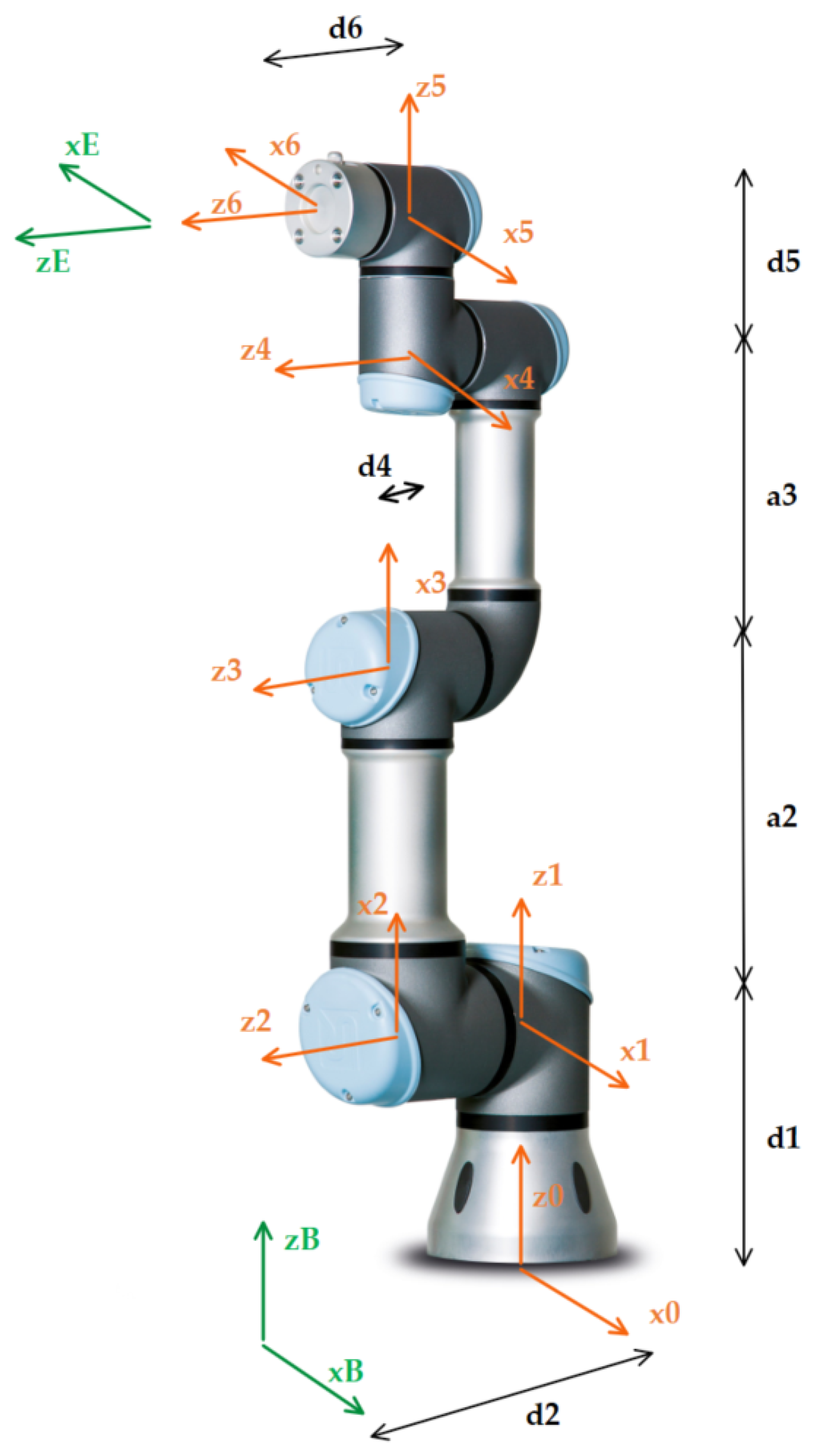
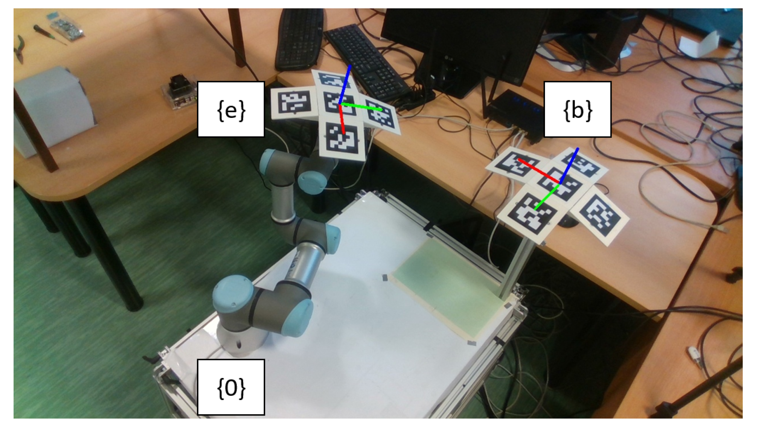
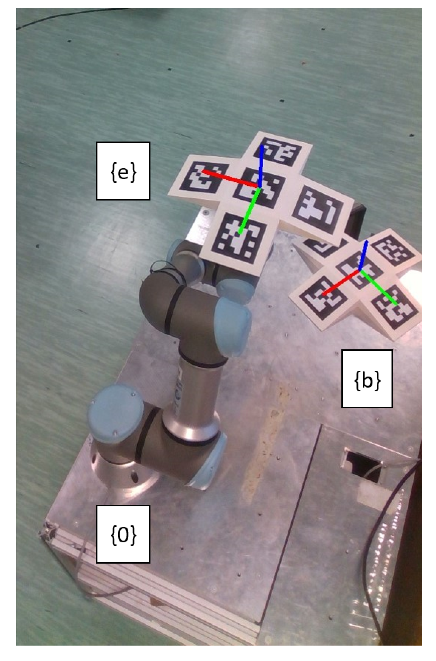
For such an identification, a geometric model that is as precise as possible of a robot needs to be determined. The Universal Robot UR3 was chosen for demonstrating the function of the proposed solution. Its geometric model used for all calculations is based on modified Denavit–Hartenberg notation (MDH), described in [22] by Craig. Our geometric model consists of 9 coordinate systems. The “b” frame is the reference coordinate system (world frame); later in our measurements it is represented by a tag marker placed on a rod. The “0” frame represents base frame of the robot. The frames from “1” to “6” represent the joints; the 6th frame position corresponds to the mounting flange. The “e” frame stands for the tool offset, in this case a measuring point that was focused by the sensor. The scheme of the model is illustrated in Figure 1. The MDH parameters are noted in

Table 1. MDH parameters of the UR3 robot.

i	${\mathit{\alpha }}_{\mathit{i}-1}$ [rad]	${\mathit{x}}_{\mathit{i}-1}$ [mm]	${\mathit{z}}_{\mathit{i}}$ [mm]	${\mathit{\theta }}_{\mathit{i}}$ [rad]	${\mathit{o}}_{\mathit{i}}$ [rad]
1	0	0	$151.90$	$q_1$	0
2	$\pi /2$	0	$119.85$	$q_2$	$\pi$
3	0	$243.65$	0	$q_3$	0
4	0	$213.25$	$-9.45$	$q_4$	0
5	$-\pi /2$	0	$83.35$	$q_5$	0
6	$\pi /2$	0	$81.90$	$q_6$	$\pi$

; the $o_i$ stands for offset of the ith joints in this position.

For a vector $q={[q_1,q_2,q_3,q_4,q_5,q_6]}^T$ representing the joint variables, a homogeneous transformation matrix $T_{be}\left(q\right)$ gives the position and orientation P of the UR3’s end-effector tool frame “e” with respect to the base frame “b” of the workplace.

$$P=T_{be}\left(q\right)$$

(1)

$$T_{be}\left(q\right)=A_{b0}{A}_{01}\left(q_1\right)A_{12}\left(q_2\right)A_{23}\left(q_3\right)A_{34}\left(q_4\right)A_{45}\left(q_5\right)A_{56}\left(q_6\right)A_{6e}$$

(2)

According to [22], matrix $A_{i-1,i}$ in MDH notation is obtained by multiplying rotation matrix $R_x$ along x axis, translation matrix $T_x$ along x axis, rotation matrix $R_z$ along z axis and translation matrix $T_z$ along z axis.

$$A_{i-1,i}=R_x\left({\alpha }_{i-1}\right)T_x\left(x_{i-1}\right)R_z\left({\theta }_i\right)T_z\left(d_i\right)$$

(3)

G=The geometric model of the UR3 is mathematically expressed by the transformation matrix $T_{be}\left(q\right)$ noted in Equation (2). Matrix $A_{b0}$ is displacement between the reference “b” frame and “0” frame; orientation difference is represented by $R_0$ rotational matrix. Matrix $A_{6e}$ is displacement between the mounting flange and “e” frame of the end-effector. The objective of this study is to determine the 12 parameters of $A_{b0}$ matrix, so to find the base frame “0” of a robot in a workplace. To be able to achieve this, it is necessary to identify during the calculations also the displacement of the end-effector ($x_e$, $y_e$, and $z_e$); however, the rotational part of the $A_{6e}$ can be freely chosen. The reason is that the transform is static (there is no variable between 6th frame of the robot and end-effector “e” frame). For simplicity, we choose $R_e$ as identity matrix.

$$A_{b0}=\left[\begin{array}{cccc}& & & x_0\\ & R_0& & y_0\\ & & & z_0\\ 0& 0& 0& 1\end{array}\right];A_{6e}=\left[\begin{array}{cccc}1& 0& 0& x_e\\ 0& 1& 0& y_e\\ 0& 0& 1& z_e\\ 0& 0& 0& 1\end{array}\right]$$

(4)

$$R_0=\left[\begin{array}{ccc}{r}_{11}& r_{12}& r_{13}\\ r_{21}& r_{22}& r_{23}\\ r_{31}& r_{32}& r_{33}\end{array}\right]$$

(5)

In general, geometric models are idealized and very difficult to make comply with real conditions due to manufacturing inaccuracy and environmental conditions. Error values can be estimated and included into the mathematical models though. Finding the relations between theoretical and real models is the crucial task of robot calibration. To find such a relation, geometric parameters of a device have to be identified. Robot identification is a process wherein error parameter values are determined using results of a test measurement. In the following simulation the UR3 robot performed a trajectory as described in Section 3. Obtained data of the end-effector position $P_c$ were compared with the robot’s position $P\left(q\right)$ based on $q_i$ for each joint.

The parameters $x_0$, $y_0$, $z_0$, $r_{11}$, $r_{12}$, $r_{13}$, $r_{21}$, $r_{22}$, $r_{23}$, $r_{31}$, $r_{32}$, $r_{33}$, $x_e$, $y_e$ and $z_e$ were chosen to be identified. The reason for identification of the end-effector frame is because the Aruco tags may be placed on a low-cost end-effector by 3D printing and the designed CAD model transformation might be different than the real solution. On the other hand, we wanted to make the model as simple as possible, so we avoided MDH parameter identification between particular joints and links of the robot, which would lead to the robot’s calibration process. We assume that this simple identification process may compensate for the small errors between the links.

When the transformation matrix $T_{be}\left(q\right)$ was defined earlier, the position vector of the end-effector P was represented by 4th column of $T_{be}$ with respect to the reference frame. If everything is ideal, we can consider this coordinate’s equal to the coordinate’s values calculated using the position sensor, as Equation (6) shows, for a specific q, where $T_{be}^{\prime }$ means 1st to 3rd elements of the 4th column of the transformation matrix.

$$P_c=T_{be}^{\prime }\left(q\right)=P\left(q\right)$$

(6)

2.2. Identification with the Jacobian Method

The most common method for parameter identification is the application of a Jacobian, which is also described, for example, in [6,16]. This iterative method utilizes benefits of the Jacobian matrix that is obtained by partial derivative of the position vector (1st to 3rd elements of 4th column) of $T_{be}$ with respect to the parameters in X, the parameters that are going to be identified. Symbolically, the Jacobian is expressed as $3\times 15$$J_i$ matrix in Equation (7), where $p_i$ stands for a parameter of X.

$$J_i=\left[\begin{array}{ccc}\frac{\partial T_{b{e}_x}(q,X)}{\partial p_1}& ...& \frac{\partial T_{b{e}_x}(q,X)}{\partial p_n}\\ \frac{\partial T_{b{e}_y}(q,X)}{\partial p_1}& \dots & \frac{\partial T_{b{e}_y}(q,X)}{\partial p_n}\\ \frac{\partial T_{b{e}_z}(q,X)}{\partial p_1}& \dots & \frac{\partial T_{b{e}_z}(q,X)}{\partial p_n}\end{array}\right]$$

(7)

For every measured point i the $J_i$ is determined. By applying all measured points a $3n\times 15$J matrix is obtained, where n is a number of measured points.

$$J=\left[\begin{array}{c}{J}_1\\ J_2\\ \dots \\ J_n\end{array}\right]$$

(8)

As a first step of every iteration a position vector $Y_m$ is calculated using values $X_j$, where j represents the iteration step. For the first iteration, guessed values $X_0$ are used. The q is the vector of joint variables measured by robot’s joint position sensors.

$$Y_m=T_{be}(q,X_i)$$

(9)

The next step is to compare and calculate the difference between the position measured by camera $Y_c$ and the previously calculated position $Y_m$, so $\Delta Y$ is determined. $Y_c$ is $n\times 3$ matrix, where n stands for number of measured points, and there are three measured coordinates $x,y,z$.

$$\Delta Y=Y_c-Y_m$$

(10)

The key equation of this method is Equation (11). When a position changes, the Jacobian matrix changes too; therefore, $\Delta x$ can be observed as the change of the parameters in X.

$$\Delta Y=J\Delta x$$

(11)

By using matrix operations in Equations (12) and (13), the values of $\Delta x$ are determined.

$${\left(J^{T}J\right)}^{-1}{J}^T\Delta Y={\left(J^{T}J\right)}^{-1}{J}^{T}J\Delta x$$

(12)

$$\Delta x={\left(J^{T}J\right)}^{-1}{J}^T\Delta Y$$

(13)

At the ends of iterations we added the computed values to the $X_{j+1}$. A convergent check follows to decide whether another iteration step is needed.

$$X_{j+1}=X_j+\Delta x$$

(14)

3. Simulations and Experiment

Two types of simulations and one experiment were performed to verify the proposed method of parameter identification. Simulation A was calculated only with absolute positions of the end-effector coordinates determined by CoppeliaSim software with the built-in UR3 model, as shown in Figure 2. The robot moved along the same path in both simulations and the experiment, consisting of 250 points. The robot stopped at each pose and the measurements were taken. The reason for choosing such a path was to obtain coordinates of the joints that were as different as possible; on the other hand, due to the experiment that was performed with cameras we needed to guarantee the visibility of the Aruco tags, which were used for the simulation B and the experiment.

3.1. Simulation A

The robot was moved along a defined path with fixed points to stop at. Once it stopped, the joint coordinates and the position vector of the end-effector related to the world base frame were acquired. With these two sets of input values, the identification was made using the methods described in the previous chapter. Results may be seen in Section 3.5.

3.2. Simulation B

For simulation B and the experiment, there were cameras and OpenCV libraries [18] applied for image processing to detect the Aruco tags. Based on the previous research by Oscadal [23], we used a 3D gridboard with tags, which improves the reliability and accuracy of detection in comparison with basic 2D tags. The gridboard represents a coordinate frame; in our case it was the base frame “b” and the end-effector frame “e” as shown in Figure 3 and Figure 4. The OpenCV library algorithm can calculate transformation from a camera to a tag. In real-time measurements, we used Equation (15) thanks to which the position of any camera was not important. Matrix $T_{cb}$ is the transformation from the camera to the base; matrix $T_{ce}$ is the transformation from the camera to the end-effector. The “c” frame is the camera frame. On the other hand, the position of a camera may be saved for later operations.

$$T_{be}=T_{cb}^{-1}{T}_{ce}$$

(15)

In the simulation B (Figure 3) we deployed the image analysis in CoppeliaSim, with a single camera of resolution 1280 × 720 px. The virtual camera was self-calibrated and the detection parameters of the OpenCV library for finding the Aruco tags were set similarly as in [23]. The dimensions of the tags were 70 × 70 mm with a 6 × 6 bit matrix.

3.3. Experiment A

Three independent cameras were placed around the UR3 robot to observe its trajectory and to calculate transformations in a laboratory during a real experiment. Intel RealSense D435i cameras with 1280 × 720 px resolution were used, and even though they are depth cameras, only the simple 2D RGB pictures were analyzed. The specifications of the cameras are shown in

Table 2. Specifications of Intel RealSense D435i camera [24].

Parameter	Value
Resolution	1920×1080 px
Frame Rate	30 fps
Sensor FOV (H × V × D)	$69.4^{\circ }\times 42.5^{\circ }\times {77}^{\circ }(\pm 3^{\circ })$
Dimensions	$90\times 25\times 25$ mm
Connection	USB‑C 3.1 Gen 1

. The cameras were self-calibrated following the methodology used in [23].

As already said before, the robot went through 250 positions on the path. To reduce the inaccuracy of the detection in reality, 10 camera frames were taken for every position, which gave us 2500 measured points. In total for the three cameras, 7500 pictures were analyzed during the calibration process.

3.4. Experiment B

To observe the impact of placement of the world base frame “b,” another experiment was performed as shown in Figure 5. Please, notice the difference in position and rotation of the base frame. Only one camera (the same type, resolution and calibration) was used in this case with robot following a similar trajectory as in the previous experiment A. The robot went through 200 poses; at each pose, five images were taken and analyzed, so 1000 measurements in total were made.

3.5. Results

The calibration results of simulations are presented in

Table 3. Results of simulations for the X vector after identification.

Parameter	Expected	Simulation A	Simulation B
$x_0$ [mm]	$431.00$	$430.98$ ($\Delta$ 0.02)	$433.59$ ($\Delta$ 2.59)
$y_0$ [mm]	$555.00$	$555.02$ ($\Delta$ 0.02)	$556.01$ ($\Delta$ 1.01)
$z_0$ [mm]	$-460.00$	$-460.07$ ($\Delta$ 0.07)	$-458.41$ ($\Delta$ 1.59)
$r_{11}$ [-]	$1.00$	$1.00$ ($\Delta$ 0.00)	$1.006$ ($\Delta$ 0.006)
$r_{21}$ [-]	$0.00$	$0.00$ ($\Delta$ 0.00)	$-0.006$ ($\Delta$ 0.006)
$r_{31}$ [-]	$0.00$	$0.00$ ($\Delta$ 0.00)	$0.001$ ($\Delta$ 0.001)
$r_{12}$ [-]	$0.00$	$0.00$ ($\Delta$ 0.00)	$0.003$ ($\Delta$ 0.003)
$r_{22}$ [-]	$1.00$	$1.00$ ($\Delta$ 0.00)	$1.004$ ($\Delta$ 0.004)
$r_{32}$ [-]	$0.00$	$0.00$ ($\Delta$ 0.00)	$-0.000$ ($\Delta$ 0.000)
$r_{13}$ [-]	$0.00$	$0.00$ ($\Delta$ 0.00)	$-0.006$ ($\Delta$ 0.006)
$r_{23}$ [-]	$0.00$	$0.00$ ($\Delta$ 0.00)	$-0.001$ ($\Delta$ 0.001)
$r_{33}$ [-]	$1.00$	$1.00$ ($\Delta$ 0.00)	$1.000$ ($\Delta$ 0.000)
$x_e$ [mm]	$0.00$	$-0.05$ ($\Delta$ 0.05)	$0.14$ ($\Delta$ 0.14)
$y_e$ [mm]	$0.00$	$-0.02$ ($\Delta$ 0.02)	$0.23$ ($\Delta$ 0.23)
$z_e$ [mm]	$66.00$	$65.98$ ($\Delta$ 0.02)	$64.78$ ($\Delta$ 1.22)

. The data calculated based on simulation A (without tag detection, only end-effector position tracking) show high-precision identification with a very small difference in comparison to the expected results (difference $\Delta$ is shown in the brackets). Such an accuracy could be achieved using, for example, a laser tracker in reality. For simulation B, when the tags were detected using simulated camera, the error was higher (maximum 2.59 mm for $x_0$), which gave us an idea about how accurate the system might be, so the noise from the environment was lowered, but the camera parameters were kept.

In

Table 4. Results of experiment A for the X vector after identification.

Parameter	Expected	Cam 1	Cam 2	Cam 3	Cameras Combined
$x_0$ [mm]	$431.00$	$432.53$	$430.81$	$426.91$	$430.05$ ($\Delta$ 0.95)
$y_0$ [mm]	$555.00$	$551.15$	$561.06$	$555.45$	$555.96$ ($\Delta$ 0.96)
$z_0$ [mm]	$-460.00$	$-451.33$	$-449.27$	$-456.496$	$-452.39$ ($\Delta$ 7.61)
$r_{11}$ [-]	$1.00$	$1.006$	$1.024$	$1.013$	$1.014$ ($\Delta$ 0.014)
$r_{21}$ [-]	$0.00$	$-0.018$	$-0.039$	$-0.015$	$-0.024$ ($\Delta$ 0.024)
$r_{31}$ [-]	$0.00$	$-0.004$	$-0.013$	$0.008$	$-0.003$ ($\Delta$ 0.003)
$r_{12}$ [-]	$0.00$	$0.020$	$0.014$	$0.007$	$0.013$ ($\Delta$ 0.013)
$r_{22}$ [-]	$1.00$	$1.008$	$1.019$	$1.004$	$1.011$ ($\Delta$ 0.011)
$r_{32}$ [-]	$0.00$	$0.000$	$-0.009$	$0.010$	$0.000$ ($\Delta$ 0.000)
$r_{13}$ [-]	$0.00$	$0.010$	$0.010$	$0.001$	$0.007$ ($\Delta$ 0.007)
$r_{23}$ [-]	$0.00$	$0.012$	$-0.009$	$-0.006$	$-0.001$ ($\Delta$ 0.001)
$r_{33}$ [-]	$1.00$	$0.990$	$0.969$	$1.011$	$0.991$ ($\Delta$ 0.009)
$x_e$ [mm]	$0.00$	$0.18$	$0.49$	$0.05$	$0.24$ ($\Delta$ 0.24)
$y_e$ [mm]	$0.00$	$0.52$	$0.73$	$0.68$	$0.65$ ($\Delta$ 0.65)
$z_e$ [mm]	$66.00$	$64.09$	$61.00$	$66.03$	$63.73$ ($\Delta$ 2.27)

are the results of the experiment A. The best values were obtained when all the results of the three cameras were combined and analyzed together. The error for the base frame ($x_0,y_0$, and $z_0$) was maximally 7.61 mm in the $z_0$ direction. We performed other measurements following the same strategy; they all provided similar results, which made it made clear that the position of a camera has an influence on the detection accuracy, which is supported by results of Krajnik’s research [25].

In

Table 5. Results of experiment B for the X vector after identification.

Parameter	Expected [mm]	Experiment B [mm]
$x_0$ [mm]	$611.00$	$613.88$ ($\Delta$ 2.88)
$y_0$ [mm]	$29.00$	$30.94$ ($\Delta$ 1.94)
$z_0$ [mm]	$-27.00$	$-25.12$ ($\Delta$ 1.88)
$r_{11}$ [-]	-	$0.506$
$r_{21}$ [-]	-	$-0.873$
$r_{31}$ [-]	-	$0.012$
$r_{12}$ [-]	-	$0.872$
$r_{22}$ [-]	-	$0.515$
$r_{32}$ [-]	-	$0.020$
$r_{13}$ [-]	-	$-0.016$
$r_{23}$ [-]	-	$-0.013$
$r_{33}$ [-]	-	$1.043$
$x_e$ [mm]	$0.00$	$-0.05$ ($\Delta$ 0.05)
$y_e$ [mm]	$0.00$	$0.69$ ($\Delta$ 0.69)
$z_e$ [mm]	$66.00$	$67.59$ ($\Delta$ 1.59)

are the results of the experiment B. It proves the possibility of placing the base frame freely with respect to the robot.

The trajectories are compared in Figure 6, Figure 7, Figure 8, Figure 9 and Figure 10. Measured cameras/measured path are plotted points that were obtained by camera/end-effector position sensor; robot path is a self-check plot of the end-effector path after the identified parameters of X were applied in the transformation matrix. Points of origin are points where the world base frame was determined for every point on the path. In Figure 11 and Figure 12 we can observe the error values in box plots.

4. Conclusions

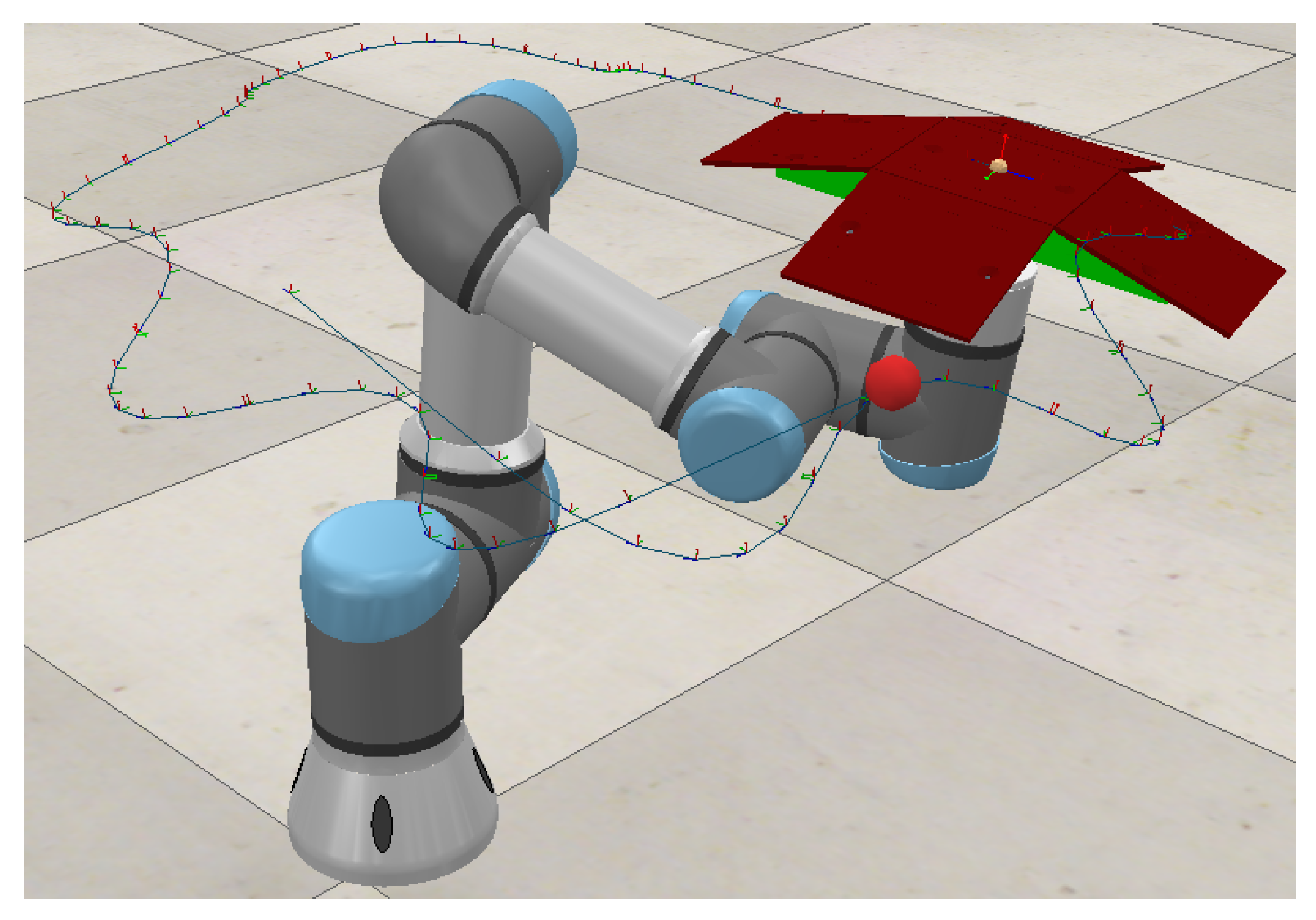
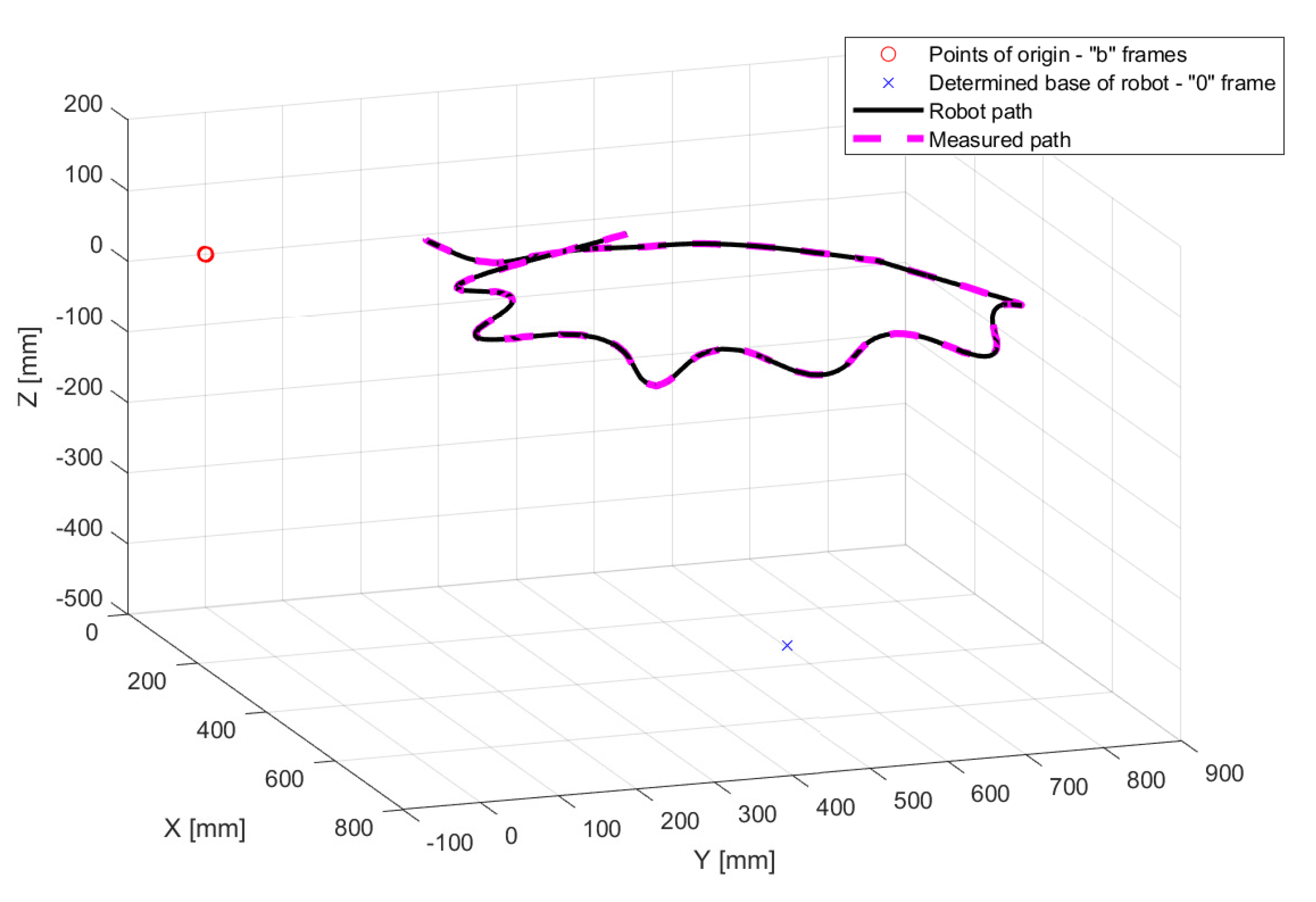
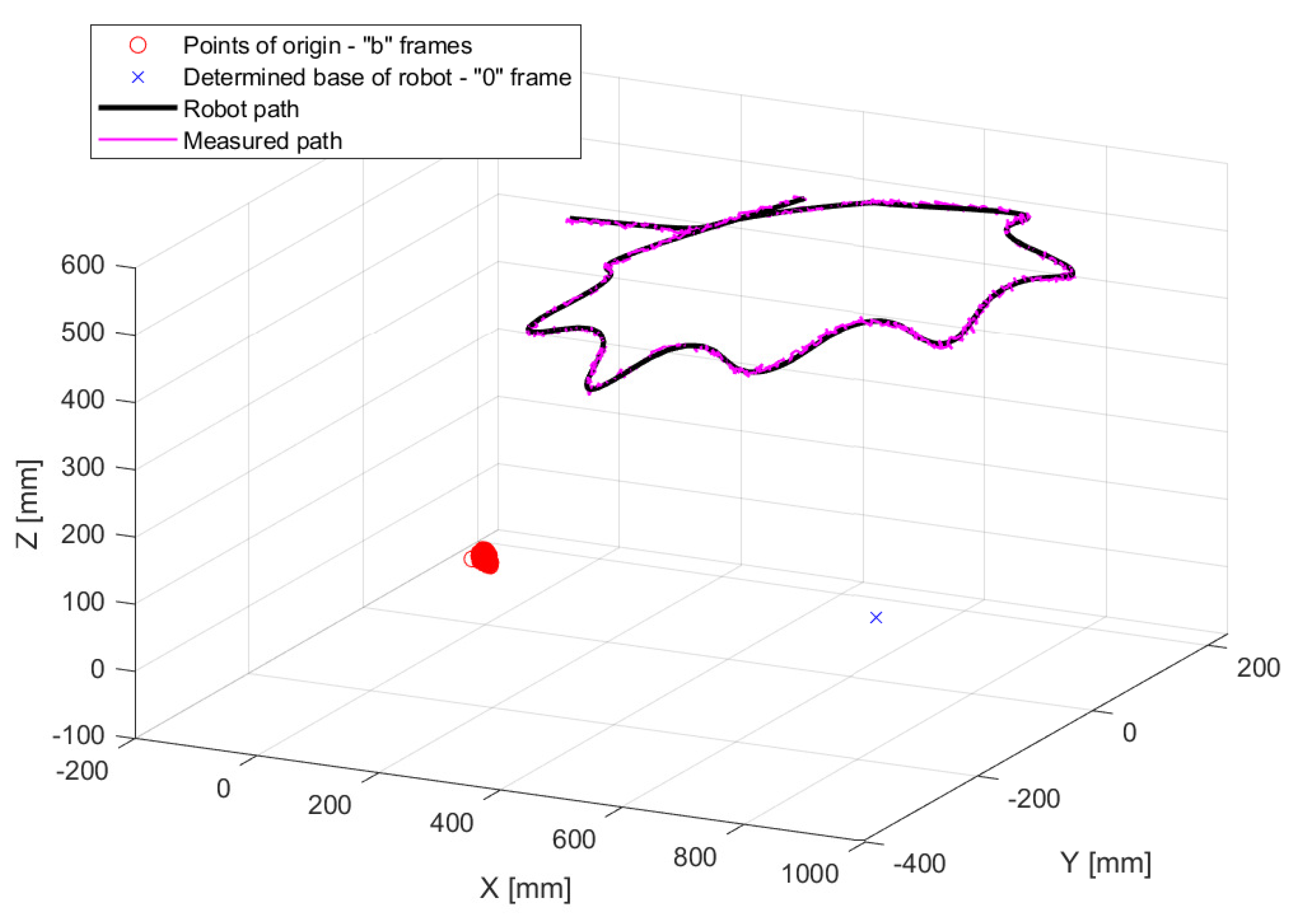
The process of identification of the robot’s base frame in a workplace using Aruco markers and OpenCV was presented and verified in this study. This approach may be used for more robots and other components of the workplace at the same time, which brings the main advantage of fast evaluation and later recalibration. The typical scenario is placing all components in their positions, placing markers on them and other points of interest, running a robot’s path while measuring end-effector position by a camera and evaluating the results—obtaining the coordinates of robot’s base and coordinates of points of interest (manipulated object, pallet, etc.). As the end-effector we used an 3D printed gridboard that might be replaced by a cubic with tags carried by a gripper.

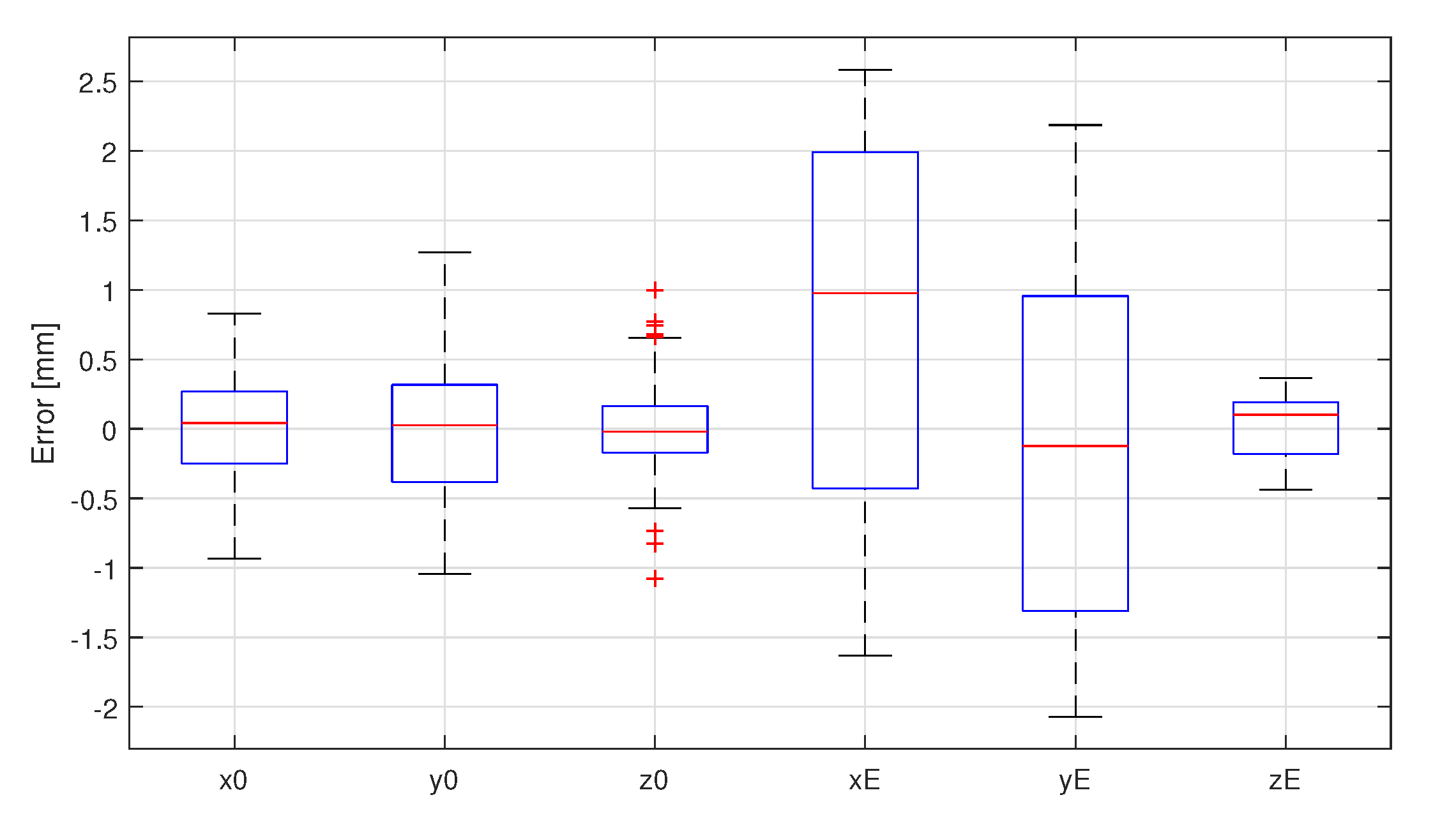
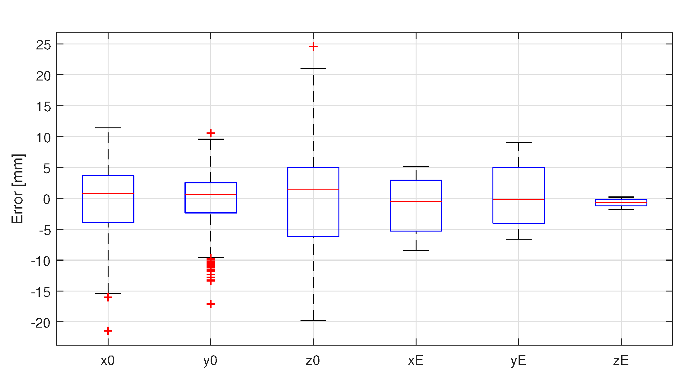
When observing the results provided in the Section 3.5, one can see there is a gap between the accuracy of the simulated workplace and the experiments. As already mentioned above, simulation A demonstrates the possible accuracy of this method when all conditions are close to ideal. Therefore, there are some methods and topics for another study that would help to minimize the errors. The DH parameters of the UR3 were based on its datasheet, but when the robot is manufactured it is calibrated and modified DH parameters are saved in the control unit. This parameters may be retrieved and applied in the identification calculations. In general, UR3 is not as precise as other industrial robots; depending on demands, a different manipulator should provide more accurate results.

Nevertheless, the end-effector was 3D printed and assembled from three parts; more accuracy may be achieved using better manufacturing methods. In some cases, if the end-effector was manufactured precisely beforehand, only the identification of a base frame might be enough (instead of identification of the base frame and end-effector offset, as was presented).

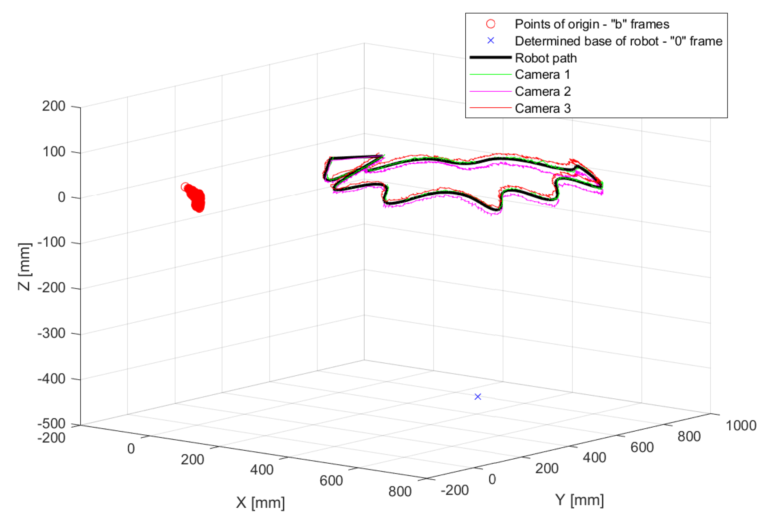
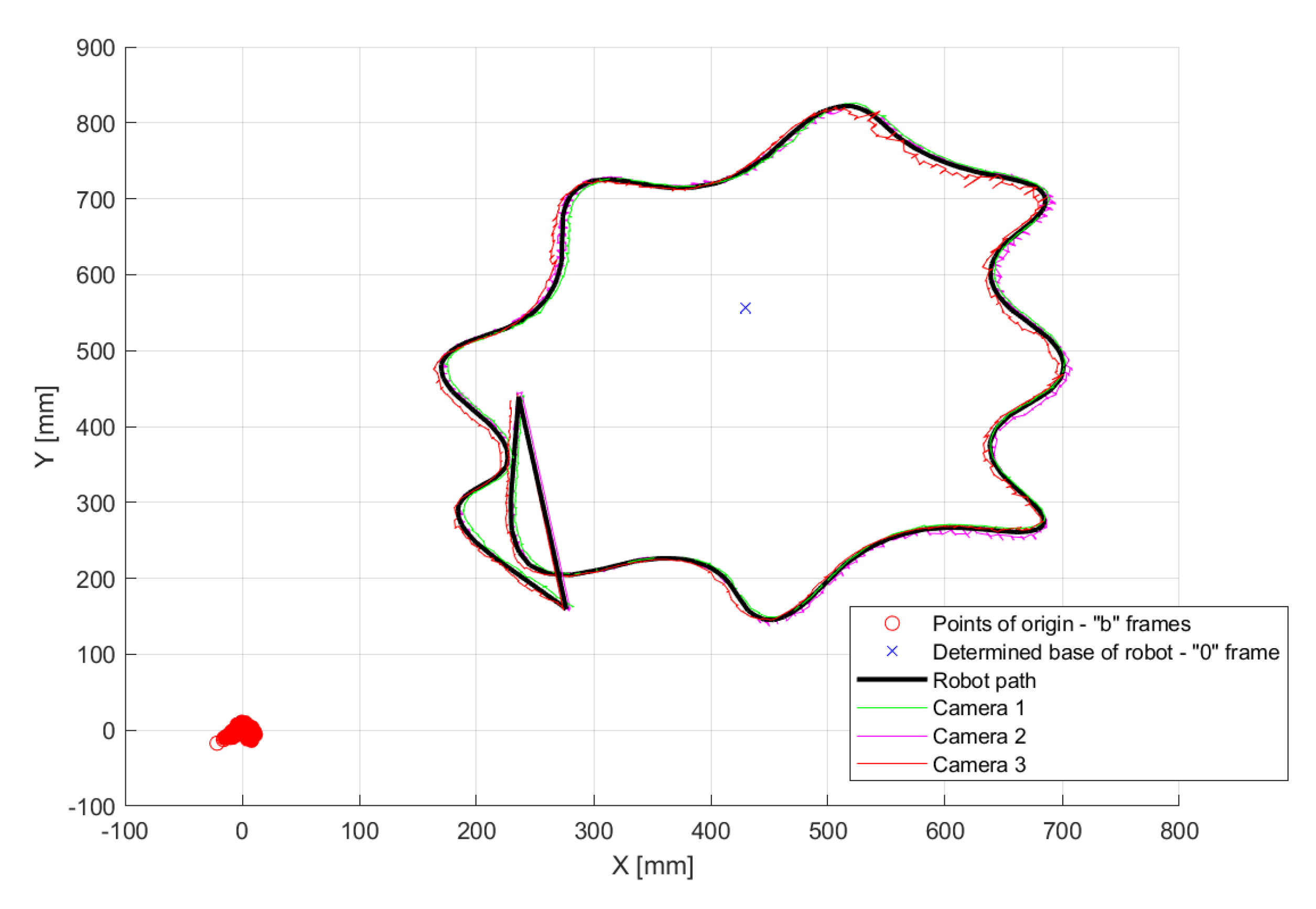
However, the biggest issue seems to be the detection of the tags, as results differed for every camera in the experiment, as shown in Table 4. Positioning of a camera (distance from a tag) seems to have a big influence on the outcome. This topic was researched in the Krajnik’s work [25]. Additionally, alternating the OpenCV’s software algorithms and filtering leads to better detection; more on this topic is discussed in [23]. A user may seriously consider the use of a self-calibrated camera with higher resolution than 1280 × 720 px, as we used. It is important to note that the presented accuracy in simulation B and real experiment were achieved by cameras that we calibrated. There is no doubt that one with better calibrated hardware may achieve more accurate results.

Another question to focus on is which trajectory and how many measured points are necessary to provide satisfying results; we tested the system with only one path of 250 points.

Once this camera-based method is well optimized for a task depending on certain available equipment, and the accuracy is acceptable, it will stand as sufficient easy-to-deploy and low-cost solution for integrators and researchers. They will be able to quickly place components and robots, tag them and obtain their position coordinates based on prepared universal measurement. In addition, even the current system may serve in the manufacturing process as a continuous safety-check that all required components, including robots, are in the place where they should be, if the detection accuracy is acceptable.

In addition, this method will be used for identification of reference coordinate systems and kinematic parameters of experimental custom manipulators, the design which is a point of interest for Research Centre of Advanced Mechatronic Systems project.

To make this calibration method easier to follow, the Matlab’s scripts with the calculations and raw input data obtained by simulation and experiments may be found on the Github page of the Department of Robotics, VSB-Technical University of Ostrava [26]. The calibration methodology and Supplementary Materials provided may serve engineers who have no previous experience with the process; they can use cameras or eventually other sensors, such as laser trackers.

References

1. Abderrahim, M.; Khamis, A.; Garrido, S.; Moreno, L. Accuracy and calibration issues of industrial manipulators. In Industrial Robotics Programming, Simulation and Application; IntechOpen: London, UK, 2004; pp. 131–146. [Google Scholar]
2. Young, K.; Pickin, C.G. Accuracy assessment of the modern industrial robot. Ind. Robot. Int. J. 2000, 27, 427–436. [Google Scholar] [CrossRef] [Green Version]
3. Slamani, M.; Nubiola, A.; Bonev, I. Assessment of the positioning performance of an industrial robot. Ind. Robot. Int. J. 2012, 39, 57–68. [Google Scholar] [CrossRef]
4. Nubiola, A.; Bonev, I.A. Absolute calibration of an ABB IRB 1600 robot using a laser tracker. Robot. Comput. Integr. Manuf. 2013, 29, 236–245. [Google Scholar] [CrossRef]
5. Wu, Y.; Klimchik, A.; Caro, S.; Furet, B.; Pashkevich, A. Geometric calibration of industrial robots using enhanced partial pose measurements and design of experiments. Robot. Comput.-Integr. Manuf. 2015, 35, 151–168. [Google Scholar] [CrossRef] [Green Version]
6. Nguyen, H.N.; Zhou, J.; Kang, H.J. A calibration method for enhancing robot accuracy through integration of an extended Kalman filter algorithm and an artificial neural network. Neurocomputing 2015, 151, 996–1005. [Google Scholar] [CrossRef]
7. Joubair, A.; Bonev, I.A. Non-kinematic calibration of a six-axis serial robot using planar constraints. Precis. Eng. 2015, 40, 325–333. [Google Scholar] [CrossRef]
8. Filion, A.; Joubair, A.; Tahan, A.S.; Bonev, I.A. Robot calibration using a portable photogrammetry system. Robot. Comput. Integr. Manuf. 2018, 49, 77–87. [Google Scholar] [CrossRef]
9. Möller, C.; Schmidt, H.C.; Shah, N.H.; Wollnack, J. Enhanced Absolute Accuracy of an Industrial Milling Robot Using Stereo Camera System. Procedia Technol. 2016, 26, 389–398. [Google Scholar] [CrossRef]
10. Lembono, T.S.; Suarez-Ruiz, F.; Pham, Q.C. SCALAR—Simultaneous Calibration of 2D Laser and Robot’s Kinematic Parameters Using Three Planar Constraints. In Proceedings of the 2018 IEEE/RSJ International Conference on Intelligent Robots and Systems (IROS), Madrid, Spain, 1–5 October 2018. [Google Scholar] [CrossRef]
11. Marie, S.; Courteille, E.; Maurine, P. Elasto-geometrical modeling and calibration of robot manipulators: Application to machining and forming applications. Mech. Mach. Theory 2013, 69, 13–43. [Google Scholar] [CrossRef] [Green Version]
12. Gan, Y.; Dai, X. Base frame calibration for coordinated industrial robots. Robot. Auton. Syst. 2011, 59, 563–570. [Google Scholar] [CrossRef]
13. Arai, T.; Maeda, Y.; Kikuchi, H.; Sugi, M. Automated Calibration of Robot Coordinates for Reconfigurable Assembly Systems. CIRP Ann. 2002, 51, 5–8. [Google Scholar] [CrossRef]
14. Motta, J.M.S.; de Carvalho, G.C.; McMaster, R. Robot calibration using a 3D vision-based measurement system with a single camera. Robot. Comput. Integr. Manuf. 2001, 17, 487–497. [Google Scholar] [CrossRef]
15. Watanabe, A.; Sakakibara, S.; Ban, K.; Yamada, M.; Shen, G.; Arai, T. A Kinematic Calibration Method for Industrial Robots Using Autonomous Visual Measurement. CIRP Ann. 2006, 55, 1–6. [Google Scholar] [CrossRef]
16. Van Albada, G.; Lagerberg, J.; Visser, A.; Hertzberger, L. A low-cost pose-measuring system for robot calibration. Robot. Auton. Syst. 1995, 15, 207–227. [Google Scholar] [CrossRef] [Green Version]
17. Santolaria, J.; Brosed, F.J.; Velázquez, J.; Jiménez, R. Self-alignment of on-board measurement sensors for robot kinematic calibration. Precis. Eng. 2013, 37, 699–710. [Google Scholar] [CrossRef]
18. Garrido, S.; Nicholson, S.; Detection of ArUco Markers. OpenCV: Open Source Computer Vision. 2020. Available online: www.docs.opencv.org/trunk/d5/dae/tutorialarucodetection.html (accessed on 23 October 2020).
19. Kroeger, O.; Huegle, J.; Niebuhr, C.A. An automatic calibration approach for a multi-camera-robot system. In Proceedings of the 2019 24th IEEE International Conference on Emerging Technologies and Factory Automation (ETFA), Zaragoza, Spain, 10–13 September 2019; pp. 1515–1518. [Google Scholar] [CrossRef]
20. Lewis, C. Industrial Calibration. 2020. Available online: https://github.com/ros-industrial/industrial_calibration (accessed on 23 October 2020).
21. Meyer, J. Robot Calibration Tools. 2020. Available online: https://github.com/Jmeyer1292/robot_cal_tools (accessed on 23 October 2020).
22. Craig, J.J. Introduction to Robotics: Mechanics and Control, 3/E; Pearson Education India: Bengaluru, India, 2009. [Google Scholar]
23. Oščádal, P.; Heczko, D.; Vysocký, A.; Mlotek, J.; Novák, P.; Virgala, I.; Sukop, M.; Bobovský, Z. Improved Pose Estimation of Aruco Tags Using a Novel 3D Placement Strategy. Sensors 2020, 20, 4825. [Google Scholar] [CrossRef] [PubMed]
24. Intel Corporation. Depth Camera D435i—Intel RealSense. 2020. Available online: https://www.intelrealsense.com/depth-camera-d435i/ (accessed on 23 October 2020).
25. Krajník, T.; Nitsche, M.; Faigl, J.; Vaněk, P.; Saska, M.; Přeučil, L.; Duckett, T.; Mejail, M. A Practical Multirobot Localization System. J. Intell. Robot. Syst. 2014, 76, 539–562. [Google Scholar] [CrossRef] [Green Version]
26. Huczala, D. Parameters Identification. 2020. Available online: github.com/robot-vsb-cz/parameters-identification (accessed on 23 October 2020).
Figure 1. UR3 with coordinate frames according to MDH.
Applsci 10 07679 g001
Figure 2. Simulated path of the UR3 in CoppeliaSim, simulation A.
Applsci 10 07679 g002
Figure 3. Simulation B with tags and a camera.
Applsci 10 07679 g003
Figure 4. Experiment A setup; point of view of camera 2.
Applsci 10 07679 g004
Figure 5. Experiment B setup.
Applsci 10 07679 g005
Figure 6. Measured path in comparison with the real robot path of simulation A.
Applsci 10 07679 g006
Figure 7. Measured path in comparison with the real robot path of simulation B.
Applsci 10 07679 g007
Figure 8. Paths measured by cameras in comparison with the real robot path of experiment A.
Applsci 10 07679 g008
Figure 9. Paths measured by cameras in comparison with the real robot path of experiment A, xy plane.
Applsci 10 07679 g009
Figure 10. Path measured by a camera in comparison with the real robot path of experiment B.
Applsci 10 07679 g010
Figure 11. Errors for the identified values based on simulation B.
Applsci 10 07679 g011
Figure 12. Errors for the identified values based on experiment A.
Applsci 10 07679 g012