Abstract
Demodulation is one of the most useful techniques for the fault diagnosis of rotating machinery. The commonly used demodulation methods try to select one sensitive sub-band signal that contains the most fault-related components for further analysis. However, a large number of the fault-related components that exist in other sub-bands are ignored in the commonly used envelope demodulation methods. Based on a weighted-empirical mode decomposition (EMD) de-noising technique and time–frequency (TF) impulse envelope analysis, a multi-scale demodulation method is proposed for fault diagnosis. In the proposed method, EMD is first employed to divide the signal into some IMFs (intrinsic mode functions). Then, a new weighted-EMD de-noising technique is presented, and different weights are assigned to IMFs for construction according to their fault-related degrees; thus, the fault-unrelated components are suppressed to improve the signal-to-noise ratio (SNR). After that, continuous wavelet transformation (CWT) is adopted to obtain the time–frequency representation (TFR) of the de-noised signal. Subsequently, the fault-related components in the entire frequency range scale are calculated together, referring to the TF impulse envelope signal. Finally, a fault diagnosis result can be obtained after the fast Fourier transformation of the TF impulse envelope signal. The proposed method and three commonly used methods are applied to the fault diagnosis of a planetary gearbox with a sun gear spalling fault and a fixed shaft gearbox with a crack fault. The results show that the proposed method can effectively detect gear faults and yields better performance than other methods.
1. Introduction
As one of the most important power transmission systems, gearboxes are widely used in many areas to provide a controlled application of power; e.g., in industrial machinery, ships, helicopters, wind turbines and automobiles [1,2,3]. A failure of the gearbox may cause the breakdown of the equipment as a whole and result in major economic losses or even disasters. Therefore, it is of great significance to detect gearbox failures as early as possible to prevent accidents from happening.
In order to detect gearbox failures, various fault diagnosis methods have been developed. Among them, vibration-based methods are attractive since vibration signals are easy to acquire and contain a great deal of gearbox health information within the signals, and they have shown good performance for diagnosing diverse gearbox failures to date [4,5]. According to theoretical studies [3,6,7,8], gearbox failures—e.g., crack, spalling and broken teeth—tend to result in abnormal vibration symptoms and create modulation phenomena in the higher-frequency range in the vibration signal, as sidebands caused by these gearbox failures are equally spaced around the modulation frequencies. Therefore, there is a need for a frequency analysis and demodulation technique to detect fault-related components from vibration signals [9].
Envelope analysis is one of the most useful demodulation techniques, and it has been widely used for the fault diagnosis of rotating machinery; e.g., bearings and gearboxes. For instance, Rubini et al. applied envelope and wavelet transform for the diagnosis of incipient faults in ball bearings; the fault diagnosis performances of different pitting failures on the outer or inner race or a rolling element were investigated [10]. McFadden presented a digital signal processing technique for calculating the amplitude and phase modulation of the tooth meshing vibration of a gear, which was applied to the early detection of local defects [11]. Wang introduced a new resonance demodulation technique to extract features related to sudden crack-induced changes in a complete revolution of a gear, which is an effective tool for the early detection of gear tooth cracks [12]. Bediaga et al. compared some traditional methods for ball bearing damage detection; the envelope analysis method was proven to be effective for localized faults on both inner and outer races [13]. Fan et al. proposed a new fault detection method that combined envelope analysis and wavelet packet transform, and it was applied to extract the modulating signal and help to detect gear faults in gearboxes at an early stage [14]. However, the traditional envelope analysis methods require band-pass filtering to capture the fault-related components, and the determination of the filter parameters requires considerable experience and expertise [15,16]. Therefore, some scholars have tried to develop improved envelope analysis methods to determine the filter parameters automatically. The fast Kurtogram method, first proposed by Antoni, has been proven to be a very powerful and practical tool for the determination of filter parameters in envelope analysis methods [17]. For instance, Zhang et al. presented a combination method based on the fast Kurtogram method and the genetic algorithm, which was successfully applied to the fault diagnosis of bearings [18]. Wang et al. proposed a time–frequency analysis method based on ensemble local mean decomposition (ELMD) and the fast Kurtogram method for rotating machinery fault diagnosis; it was successfully implemented in the fault diagnosis of both bearings and a gearbox [19]. Lei et al. introduced an improved Kurtogram method that adopted wavelet packet transformation (WPT) as the filter banks of the Kurtogram method, which was verified to be an effective method for diagnosing faults in rolling element bearings [20]. Wang et al. proposed an enhanced Kurtogram method for the fault diagnosis of bearings, where kurtosis values were calculated based on the power spectrum of the envelope of the signals extracted from wavelet packet nodes at different depths; their method was proven to be effective for the detection of various bearing faults [21].
Above all, the traditional envelope analysis and fast Kurtogram methods have been effectively applied to the fault diagnosis of bearings and gearboxes. However, most of these approaches try only to select one sensitive sub-band scale signal that contains the most fault-related components for further analysis, and a large number of fault-related components that exist in other sub-bands are ignored, which may lead to a degradation of the fault diagnosis result, especially at the early stage of a fault. Therefore, a robust multi-scale demodulation method based on the weighted-EMD de-noising technique and time-frequency impulse envelope analysis is proposed; the fault-related components in the entire frequency range scale are extracted for further analysis. A planetary gearbox with a sun gear spalling fault and a fixed shaft gearbox with a crack fault are used to demonstrate the effectiveness of the proposed method.
The rest of the paper is organized as follows. Section 2 discusses the physical mechanisms of the modulation phenomenon of a gearbox based on the dynamic simulation method. Section 3 introduces the detailed procedure of the proposed robust multi-scale demodulation method. Then, in Section 4 and Section 5, experimental studies on a planetary gearbox with a seeded sun gear spalling fault and a fixed shaft gearbox with a crack fault are conducted to confirm the effectiveness of the proposed method. Finally, concluding remarks are provided in Section 6.
2. Problem Formulation
In the fault diagnosis of gearboxes, it is known that modulation phenomena will be observed in vibration signals when there is a gear fault in a gearbox [22,23]; e.g., amplitude modulation (AM) and frequency modulation (FM). In order to improve the success rate of the fault diagnosis method, it is necessary to determine the physical mechanism of the modulation phenomena caused by gear faults.
Figure 1a presents a schematic diagram of a gear pair with a local tooth fault; except for the faulty tooth, the other teeth of the pinion correspond to normal meshing. Figure 1b compares the stiffnesses of the normal and faulty gear mesh, which are calculated based on an analytical method [6,7,8]. It can be seen that there is a sudden reduction of the gear mesh stiffness when the faulty tooth is engaged; thus, a periodic reduction of gear mesh stiffness will be observed in each revolution of the pinion.
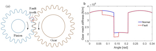
Figure 1.
Schematic diagram of (a) a gear pair with a local tooth fault and (b) comparison between normal and fault gear mesh stiffnesses.
In order to study the modulation mechanism of the vibration signals caused by the periodic reduction of gear mesh stiffness, a six degrees-of-freedom (6 DOFs) lumped parameter model for a gear system is established; the schematic diagram of the spur gear system is shown in Figure 2. means the inertial moment; mi is the mass; and stand for the stiffness of the support bearings in the x direction and y direction, respectively; and are the damping of the support bearings in the x direction and y direction, respectively; is the inter-tooth friction force; is the torque; is the rotating speed; represents the time-varying mesh stiffness; is the mesh damping between gear teeth; and i = p, g for the pinion and gear, respectively. The governing equations of the gear system can be obtained as follows:
where denotes the angular acceleration; , and stand for displacement, velocity and acceleration in the x direction, ; and refer to the displacement, velocity and acceleration in the y direction; means the normal mesh force moment; is the friction force moment; and N is the net contact force due to the elasticity. The subscript i = p, g for the pinion and gear, respectively.
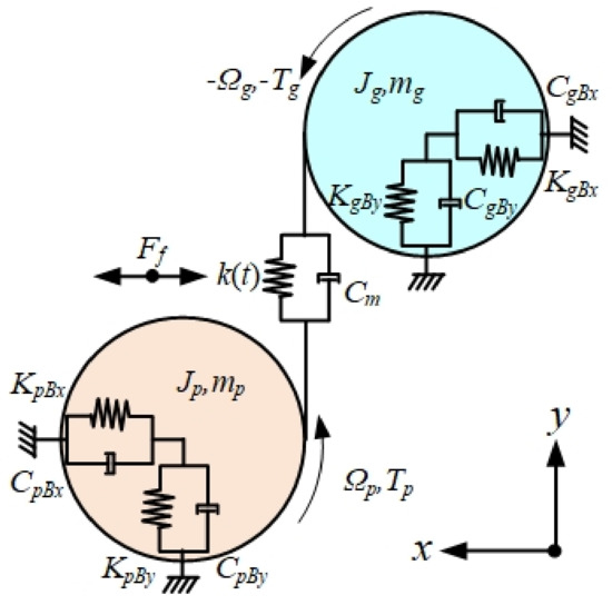
Figure 2.
Schematic diagram of gear system with six degrees-of-freedom (6 DOFs).
Figure 3 illustrates the simulated waveform of the dynamic transmission error (DTE) of the gear system with a local tooth fault and its corresponding spectrum. It is observed that there is a periodic impulse caused by the tooth fault, and the cycle equals 2. Furthermore, abundant modulation sidebands are found around the meshing frequency and its harmonics, as shown in Figure 3b. Then, the variation of the order spectrum corresponding to the rotating speeds is simulated and plotted, as shown in Figure 4. It is found that there are many modulated sidebands around the dotted line in each rotating speed, and the frequency range of the sub-bands are time-varying with respect to the rotating speeds. However, there are also some sub-bands that contain the fault-related components, as shown by the oval area in Figure 4, which are defined as multi-scale modulation phenomena in this paper.
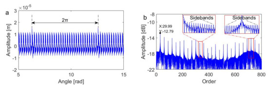
Figure 3.
(a) Waveform of the dynamic transmission error (DTE) of the gear system with a local tooth fault and (b) its corresponding order spectrum at a speed condition of 30 rad/s.
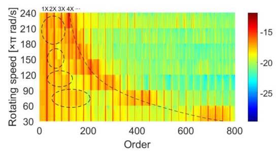
Figure 4.
Variation of the order spectrum corresponding to the rotating speeds.
Therefore, if a large number of the fault-related components that exist in other sub-bands are ignored in the demodulation analysis, this may lead to the degradation of the fault diagnosis result, especially at the early stage of a fault.
3. The Proposed Multi-Scale Demodulation Method
The main principle behind the proposed method is to extract the fault-related components that exist in the entire frequency range of the vibration signals. In the proposed method, there is no need to search for the variable optimal modulation sub-bands due to the variable rotating speeds. However, vibration signals are usually composed of multiple components; e.g., fault-related components, background noise and interference from other normal machinery parts. Therefore, it is important to remove the noise components and interference components from the raw vibration signals to improve the quality of the extracted impulsive shocks. It is known that the EMD method can decompose a signal into some mono-components self-adaptively, and these mono-components are nearly orthogonal according to [24,25]. Therefore, the fault-related components, background noise, interference, etc., can be decomposed and further processed.
3.1. Adaptive Signal Decomposition Based on EMD
The EMD method was first proposed by Huang et al. in 1998 [24]. It can decompose a signal into some mono-components according to the local characteristic time scales of the signal—so-called intrinsic mode functions (IMFs)—to represent the natural oscillatory mode embedded in the signal and work as the basis functions; the method can be applied to nonlinear and non-stationary processes. The detail procedure of EMD is given as follows.
Step 1: Calculation of the envelope.
Identify all the local extrema in the signal. Connect all the local maxima by a cubic spline line as the upper envelope. Repeat the procedure for the local minima to produce the lower envelope. The schematic plot is as shown in Figure 5.

Figure 5.
Schematic plot of the calculation of upper and lower envelopes.
Step 2: Removal of the envelope mean.
Calculate the mean of the upper and lower envelopes. Remove these from the signal .
Step 3: Extraction of the IMF.
To judge whether is an IMF, if satisfies the requirements of an IMF, set the first IMF as = . Otherwise, let be the raw signal, and repeat step 1 to step 2. It is noted that an IMF is defined as a function that satisfies the following requirements: (1) in the whole data set, the number of extrema and the number of zero-crossings must either be equal or differ at most by one; (2) at any point, the mean value of the envelope defined by the local maxima and the envelope defined by the local minima is zero.
Step 4: Decomposition. Separate the IMF from the raw signal .
where the residual signal is treated as the raw signal = and subjected to the same sifting process from step 1 to step 3; then, the second IMF can be obtained. After n repeats, the sifting process finally stops when the residue becomes a monotonic function from which no more IMFs can be extracted.
Thus, a decomposition of the signal into n-empirical modes is achieved. The IMF from to carries oscillating components of the raw signal from high frequency to low frequency.
3.2. Time–Frequency Representation (TFR) Calculation Based on Continuous Wavelet Transformation (CWT)
TFR analysis methods are applied to study a signal in both the time and frequency domains simultaneously. Among the commonly used TFR calculation methods, CWT has been proven to be powerful for the analysis of non-stationary signals; it offers good frequency resolution at low frequencies and good time resolution at high frequencies. The application of CWT for mechanical fault diagnosis has attracted a great deal of attention over the past decades [26,27,28]. The detailed procedure of CWT is summarized as follows.
Suppose is an energy signal, namely ; then, the wavelet transformation of is defined as the integral of the kernel function with .
where is obtained from the wavelet function by expansion and translation.
where is the scale parameter, b is the location parameter and is the normalized constant factor to ensure the conservation of the signal energy. When a decreases, the time width of the wavelet function decreases and the frequency bandwidth increases; on the contrary, the frequency bandwidth of the wavelet function decreases and the time width increases. Therefore, CWT can yield good frequency resolution at low frequencies and good time resolution at high frequencies.
Wavelet transform can be seen as a re-expression of the signal at different scales of the wavelet basis. Thus, the selection of the wavelet basis function has a direct effect on the TFR quality. A good wavelet basis function can match the impulsive shocks caused by machinery fault well and suppress the background noise. A Morlet wavelet is a double-side wavelet, which has been proven to be useful in the fault diagnosis of gearboxes and bearings [29,30,31]. It is defined in the time domain as follows, and the corresponding waveform is as shown in Figure 6.
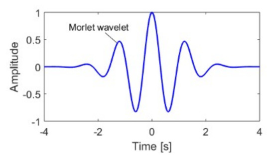
Figure 6.
Waveform of the Morlet wavelet.
3.3. Fault Diagnosis Procedure Based on the Proposed Method
The detailed fault diagnosis procedure based on the proposed method is shown in Figure 7. The raw vibration signal is first acquired from the machinery. Then, the EMD method is applied to decompose the raw vibration signal into n IMFs, denoted as , , …, . Different IMFs have different sensitivities to fault-related components. In order to choose the most fault-related IMF and suppress the fault-unrelated IMFs, a weighted-EMD de-noising technique is presented based on Pearson’s correlation analysis and a weighting method.
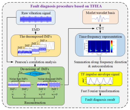
Figure 7.
Fault diagnosis procedure based on the proposed method.
First, the correlation coefficients between the raw vibration signal and different IMFs are calculated [32,33],
where x refers to the raw vibration signal, is the mean of x, K equals the length of x, stands for the ith IMF and is the mean of . Then, IMFs are partitioned into noise-free IMFs and noise-dominant IMFs with a given threshold.
The reconstructed signal can be obtained from the noise-free and noise-dominant IMFs after a weighting process.
where refers to the weight of the ith IMF.
where denotes the correlation coefficient vector of n IMFs. indicates the given threshold for IMF grouping; in this paper, it is chosen as the mean value of as an example to study the effectiveness of the proposed method.
After that, CWT is carried out to obtain the TFR of the reconstructed signal. Then, the time-frequency impulse envelope signal can be calculated from the through a summation along the frequency direction. Furthermore, autocorrelation is performed to to improve the signal-to-noise ratio. Finally, the time–frequency impulse envelope spectrum can be obtained for fault diagnosis after fast Fourier transformation.
where refers to the sampling frequency, is the Nyquist frequency and l means the time lag.
Above all, the fault-related components can be demodulated according to the proposed method, and there is no need to select optimal sub-band signals for different rotating speed conditions.
4. Validation of the Proposed Method by the Fault Diagnosis of a Planetary Gearbox with a Sun Gear Spalling Fault
4.1. Description of the Experimental System
The planetary gearbox (PGB) experimental test rig is shown in Figure 8. It consisted of two planetary gearboxes, two motors, an industrial computer and a control box, which were arranged symmetrically. The detailed design parameters of the planetary gearbox are given in Table 1, and the schematic of PGB is depicted in Figure 9. It contained four planet gears, a standstill ring gear, a sun gear and a carrier. In PGB 1, the sun gear was the input and the carrier was the output; in PGB 2, the carrier was the input and the sun gear was the output. The seeded sun gear tooth spalling fault was located in PGB 1; the schematic diagram and the photograph of the spalling fault are shown in Figure 10. The spalling fault’s length equalled 35 mm, the width equalled 4 mm and the depth equalled 2 mm. The power of the two Siemens three-phase induction motors was 15 kW; motor 1 is for driving and motor 2 is for loading.
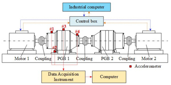
Figure 8.
The planetary gearbox (PGB) experimental test rig.

Table 1.
Design parameters of the planetary gearbox.
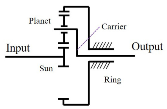
Figure 9.
Schematic of PGB.
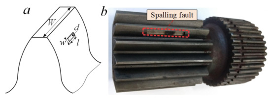
Figure 10.
The seeded spalling fault: (a) schematic diagram, (b) photograph.
Four ICP accelerometers were mounted in the housing of PGB 1 to acquire vibration signals, denoted as ♯1, ♯2, ♯3 and ♯4, respectively. ♯1 was placed in the housing of the input bearing, ♯2 was placed in the planetary gearbox base, ♯3 was placed in the ring gear of the planetary gearbox and ♯4 was placed in the housing of the carrier bearing, as illustrated in Figure 8. An LMS SCADAS SC305 (a Siemens data acquisition instrument) was applied for data acquisition; the sampling frequency was set as 20,480 Hz, and the sampling length was set as 11 s. Three datasets were acquired with rotating speeds equal to 100 rpm, 300 rpm and 500 rpm, respectively; it is noted that the vibration signals of ♯4 are analyzed in this study.
The corresponding characteristic frequencies of the planetary gearbox are calculated with the equation in [34] and given in Table 2.
where , and indicate the tooth number of sthe un gear, ring and planet gear, respectively. is the number of the planet gear. , and are the rotating frequencies of the sun gear, carrier and planet gear, respectively; refers to the meshing frequency; and is the fault characteristic frequency.
Table 2.
Characteristic frequencies of the planetary gearbox.
4.2. Results and Discussion
The time waveforms and the corresponding spectra of the planetary gearbox under 100 rpm, 300 rpm and 500 rpm rotating speeds are shown in Figure 11. It can be found that several obvious impulsive shocks were caused by the spalling fault, as shown in Figure 11a–c, and the impact frequency and the amplitude of impulsive shocks became larger when the rotating speed increased from 100 rpm to 500 rpm. Besides, there were also some changes of the spectrum, as shown in Figure 11d–f. Under a 100 rpm working condition, the dominant frequencies of the spectrum were 224.1 Hz and 1087 Hz. Under a 300 rpm working condition, the dominant frequencies of the spectrum were 213 Hz and 1208 Hz. Under a 500 rpm working condition, the dominant frequencies of the spectrum were 448 Hz and 1345 Hz, and more obvious sidebands could be found.
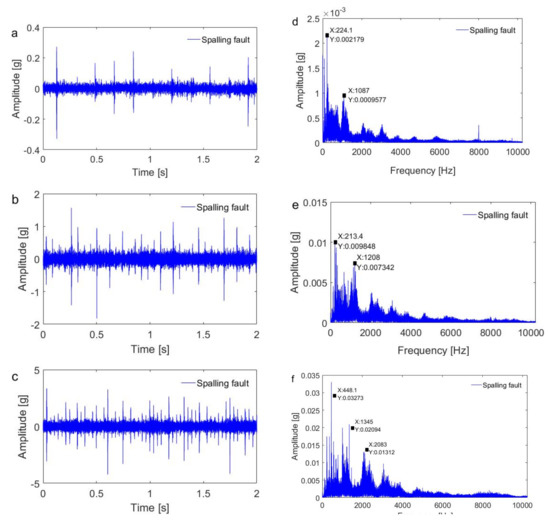
Figure 11.
Time waveforms of a planetary gearbox under (a) 100 rpm, (b) 300 rpm and (c) 500 rpm working conditions and the corresponding spectra under (d) 100 rpm, (e) 300 rpm and (f) 500 rpm working conditions.
Figure 12a–c illustrates the TFR of the vibration signal after the denoising process for 100 rpm, 300 rpm and 500 rpm conditions, respectively. It can be found that impulsive shocks can be observed clearly in the TFRs of vibration signals, and the impulsive shocks became more intensive as the rotating speed increased from 100 rpm to 500 rpm. The frequency range of these impulsive shocks also became wider as the rotating speed increased; under the 100 rpm working condition, the impulsive shocks were present in a frequency range below 4000 Hz, while under the 500 rpm working condition, the impulsive shocks were present over almost the entire frequency range.
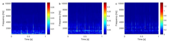
Figure 12.
Time–frequency representation (TFR) of the planetary gearbox vibration signal after the denoising process: (a) TFR at 100 rpm, (b) TFR at 300 rpm and (c) TFR at 500 rpm.
According to the proposed method, both the time–frequency impulse envelope waveforms and the corresponding demodulation spectra could be calculated based on the TFR of the vibration signals, as shown in Figure 13. The impulse envelope waveforms of the three datasets are shown in Figure 13a–c. The corresponding demodulation spectra of the three datasets are shown in Figure 13d–f. Under the 100 rpm working condition, five impulsive shocks caused by the spalling fault were found, as shown in Figure 13a. The sun gear fault characteristic frequency of 5.625 Hz and its harmonics could be observed clearly in the demodulation spectrum, as shown in Figure 13d. Under a 300 rpm working condition, 17 impulsive shocks caused by the spalling fault were found, as shown in Figure 13b. The sun gear fault characteristic frequency of 16.88 Hz and its harmonics could be observed clearly in the demodulation spectrum, as shown in Figure 13e. Similarly, 28 impulsive shocks caused by the spalling fault were found in the 500 rpm working condition, as shown in Figure 13c. The sun gear fault characteristic frequency of 28.13 Hz and its harmonics could be observed clearly in the demodulation spectrum, as shown in Figure 13f. The conclusion can be drawn that the proposed method can accurately extract the modulation components caused by a spalling fault without the selection of variable optimal modulation sub-bands under different rotating speed conditions.
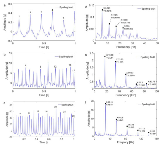
Figure 13.
Impulse envelope waveforms under (a) 100 rpm, (b) 300 rpm and (c) 500 rpm working conditions and the corresponding demodulation spectra under (d) 100 rpm, (e) 300 rpm and (f) 500 rpm working conditions.
The original fast Kurtogram proposed by Antoni [15], the enhanced Kurtogram proposed by Wang et al. [19] and the traditional envelope analysis method were applied to analyze the same datasets for comparison.
The demodulation results based on the fast Kurtogram method are shown in Figure 14. The fast Kurtograms of the three datasets are shown in Figure 14a–c. The corresponding demodulation spectra of the three datasets are shown in Figure 14d–f. Under the 100 rpm working condition, the optimal demodulation scale chosen by the fast Kurtogram was at level 4, and the frequency ranged from 1920 to 2560 Hz, as shown in Figure 14a. The corresponding demodulation spectrum is shown in Figure 14d; the fault characteristic frequency and its harmonics were not as clear as the proposed method, and there were many noise components. Under the 300 rpm working condition, the optimal demodulation scale chosen by the fast Kurtogram method was at level 3.6 and the frequency ranged from 4266.5 to 5119.5 Hz, as shown in Figure 14b. The corresponding demodulation spectrum is shown in Figure 14b; it is also difficult to observe the fault characteristic frequency and its harmonics due to the noise components. Under the 500 rpm working condition, the optimal demodulation scale chosen by the fast Kurtogram method was at level 4 and the frequency ranged from 1920 to 2560 Hz, as shown in Figure 14c. The corresponding demodulation spectrum is shown in Figure 14d; it is observed that the fault characteristic frequency of 28.13 Hz and its harmonics could be found, although it contained more noise components compared to the time–frequency impulse envelope demodulation result in Figure 14f.
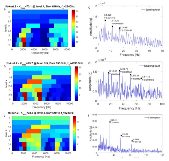
Figure 14.
Fast Kurtograms under (a) 100 rpm, (b) 300 rpm and (c) 500 rpm working conditions and the corresponding demodulation spectra under (d) 100 rpm, (e) 300 rpm and (f) 500 rpm working conditions.
The demodulation results based on the enhanced Kurtogram method are shown in Figure 15. The enhanced Kurtograms of the three datasets are shown in Figure 14a–c. The corresponding demodulation spectra of the three datasets are shown in Figure 15d–f. It can be found the optimal demodulation scales chosen by the enhanced Kurtogram method were all at wavelet packet node (4, 3) for the three working conditions; the frequency ranged from 1920 to 2560 Hz. Under the 100 rpm working condition, the fault characteristic frequency of 5.625 Hz and its harmonics could be found as shown in Figure 15d, but it contained more noise components compared to the time–frequency impulse envelope demodulation result in Figure 13d. Under the 300 rpm working condition, the fault characteristic frequency of 16.88 Hz and its harmonics could be found as shown in Figure 15e; it also contained more noise components compared to the time–frequency impulse envelope demodulation result in Figure 13e. Similarly, under the 500 rpm working condition, the fault characteristic frequency of 28.13 Hz and its harmonics could be found as shown in Figure 15f; it also contained more noise components than the time–frequency impulse envelope demodulation result in Figure 13f. In summary, the enhanced Kurtogram method yielded better results than the fast Kurtogram method but contained more noise components than the proposed method.
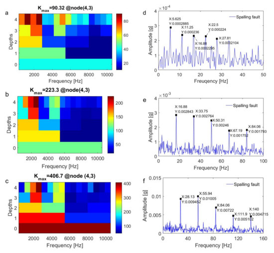
Figure 15.
Enhanced Kurtograms under (a) 100 rpm, (b) 300 rpm and (c) 500 rpm working conditions and the corresponding demodulation spectra under (d) 100 rpm, (e) 300 rpm and (f) 500 rpm working conditions.
The demodulation results based on the traditional envelope analysis method are shown in Figure 16; the demodulation sub-bands were chosen depending on experience. Under the 100 rpm working condition, the demodulation sub-band was chosen at around a 10× meshing frequency to include the dominant frequency of the spectrum in Figure 11d—specifically, from 120 to 320 Hz—and it was observed that only the fault characteristic frequency of 5.625 Hz could be found, as shown in Figure 16a. Under the 300 rpm working condition, the demodulation sub-band was chosen around a 4× meshing frequency to include the dominant frequency of the spectrum in Figure 11e—specifically, from 170 to 370 Hz—and it was observed that there were no fault-related components in the demodulation spectrum, as shown in Figure 16b. Under the 500 rpm working condition, the demodulation sub-band was also chosen at around a 4× meshing frequency to include the dominant frequency of the spectrum in Figure 11f—specifically, from 350 to 550 Hz—and it was observed that there were also no fault-related components in the demodulation spectrum, as shown in Figure 16c.
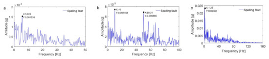
Figure 16.
Demodulation spectra based on traditional envelope analysis under (a) 100 rpm, (b) 300 rpm and (c) 500 rpm working conditions.
In order to validate the superiority of the proposed method to the other three methods, the mean–peak ratio () index [35] was applied to measure the fault-related components in the demodulation spectrum. A higher value indicates a better demodulation performance. is defined as follows,
where indicates the number of harmonics of the fault characteristic frequency needed to compute an , which is set as 5 in this study, and is the amplitude of the spectral peak around the ith harmonic of the fault characteristic frequency. As the average value of the spectral components is in the range from a Hz to b Hz, is the amplitude of the kth spectral component.
Figure 17 illustrates the values of the four methods in different working conditions. It can be observed that the proposed method always achieved higher values under the three working conditions. It yielded an average gain of 27.48 dB compared to the fast Kurtogram method, an average gain of 16.33 dB compared to the enhanced Kurtogram method and an average gain of 33.01 dB compared to the traditional envelope analysis method, respectively. This is mainly because the proposed method retains more fault-related components in the entire frequency range scale and the weighted-EMD de-noising technique effectively removes the noise components and interference components from the raw vibration signals.
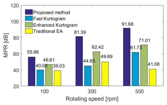
Figure 17.
Mean–peak ratio () values of the four methods under 100 rpm, 300 rpm and 500 rpm rotating speed conditions.
Moreover, the effect of the given threshold in the weighted-EMD de-noising technique on the demodulation performance of the proposed method was discussed, as shown in Figure 18. It was found that the peaks were reached when the thresholds equalled 2.5, 1.5 and 2 under the three working conditions, respectively. However, it was also observed that there was a sudden drop of the value when the given threshold was too large. This was because some fault-related components were recognized as noise components when the threshold was too large.
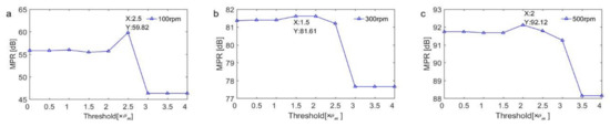
Figure 18.
Effect of the given threshold in the weighted-EMD de-noising technique on demodulation performance under (a) 100 rpm, (b) 300 rpm and (c) 500 rpm working conditions.
5. Validation of the Proposed Method by the Fault Diagnosis of a Fixed Shaft Gearbox with a Seeded Tooth Root Crack Fault
5.1. Description of the Experimental System
The experimental test for the fixed shaft gearbox with a seeded tooth root crack fault is shown in Figure 19. The setup consisted of an industrial computer, a three-phase motor, a two-stage gearbox (transmission ratio = 3.59), a torque sensor, a magnetic particle brake and several elastic couplings. The industrial computer controlled the three-phase motor with a frequency converter to realize the simulation of different speeds, and the load controller controlled the magnetic particle brake to realize the simulation of different loads. The first-stage gear ratio was 23/39 and the second-stage gear ratio was 25/53. The tooth root crack fault was seeded by wire cutting, involving a penetrating crack with a depth of 2 mm and a cutting angle of 70 degrees. The faulty gear was installed on the intermediate shaft, as shown in Figure 20. The seeded tooth root crack fault gear was mounted on the second pair of gear engagement pairs of the gearbox intermediate shaft. The speed increased from 500 rpm to 700 rpm and then decreased to 500 rpm with a load of 0 Nm. The characteristic frequency of the gearbox at 500 rpm and 700 rpm is shown in Table 3. The signal sampling frequency was 5120 Hz and the sampling length was 32 s.
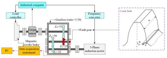
Figure 19.
The seeded tooth root crack fault.
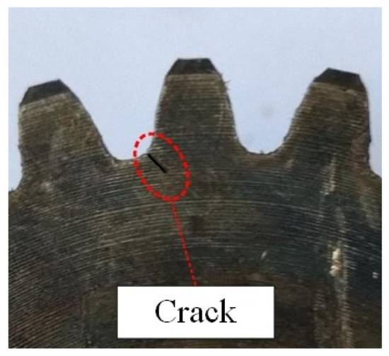
Figure 20.
The seeded tooth root crack fault.
Table 3.
Characteristic frequencies of the fixed shaft gear train.
5.2. Results and Discussion
The vibration signal waveform of the gearbox while increasing and decreasing speed is shown in Figure 21. It could be found that the amplitude of the gearbox vibration had the same change trend as the increase and decrease of speed. We selected 500 rpm data in the initial stage and 700 rpm data in the intermediate stage to verify whether the algorithm could extract the fault characteristic vibration adaptively. The data interception time was 2 s, assuming that the vibration data in 2 s was quasi-static. The time-domain waveforms and spectra of vibration signals at 500 rpm and 700 rpm operating conditions are shown in Figure 22. Through analysis, it could be found that the spectrum structure changed to a certain extent as the operating condition increased from 500 rpm to 700 rpm. At 500 rpm, the energy mainly concentrated near 383.4 Hz, 725.6 Hz and 1745 Hz. At 700 rpm, the energy mainly concentrated around 536.6 Hz, and the spectrum energy distribution drifted.
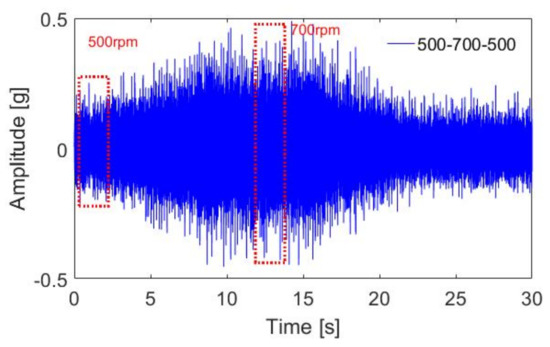
Figure 21.
Vibration waveform of the gearbox under working conditions of increasing and decreasing speed.
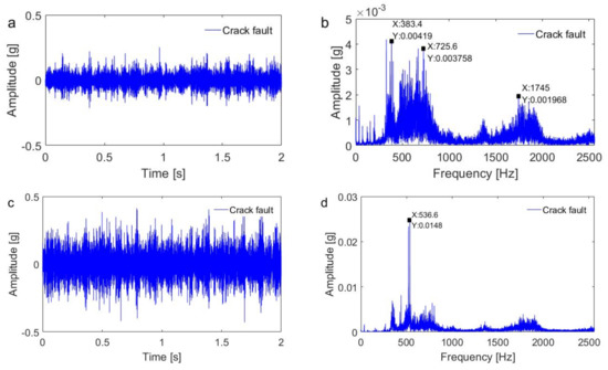
Figure 22.
Vibration waveform and spectrum of the gearbox in two working conditions: (a) time-domain waveform under the 500 rpm condition, (b) frequency spectrum under the 500 rpm condition, (c) time domain waveform under the 700 rpm condition, (d) frequency spectrum under the 700 rpm condition.
Based on the decomposition and reconstruction of the weighted-EMD, the time–frequency distribution of the vibration signals of gearbox under 500 rpm and 700 rpm operating conditions was calculated as shown in Figure 23a,b. It could be found that the impact components of the time–frequency vibration caused by the root crack fault were more disordered than those caused by the sun wheel flaking fault test, but impact characteristics of comparative regularity could still be found. When the working condition increased from 500 rpm to 700 rpm, the energy of the impact component increased and the time interval became shorter.
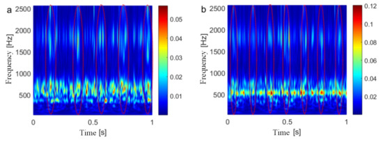
Figure 23.
Comparisons of the time–frequency distribution of the gearbox vibration signal between the two working conditions: (a) 500 rpm, (b) 700 rpm.
The time–frequency shock envelope characteristic signals and their demodulation spectra under two conditions were extracted and calculated as shown in Figure 24. At 500 rpm, the extracted time–frequency impulse characteristic signal was as shown in Figure 24a. Five impulse components were clearly visible within one second, and the corresponding impulse demodulation spectra were clearly visible at 5 Hz and 10 Hz, which corresponded to the local fault characteristic frequency of the solar wheel and its 2× harmonic frequency, respectively, as shown in Figure 24b. At 700 rpm, the extracted time–frequency impulse characteristic signal was as shown in Figure 24c. Seven impulse components were clearly visible in one second, and the corresponding impulse demodulation spectra were 6.875 Hz, 13.75 Hz and 20.63 Hz, which corresponded to the local fault characteristic frequency and second-order and third-order harmonic frequencies of the solar wheel, respectively, as shown in Figure 24d.

Figure 24.
Impulse envelope signal under (a) 500 rpm, (c) 700 rpm working conditions and the demodulation spectra under (b) 500 rpm, (d) 700 rpm working conditions.
Based on the fast Kurtogram method, the performance of the demodulation spectrum under the two conditions was analyzed as shown in Figure 25. Under the 500 rpm operating condition, the optimum demodulation scale selected by the fast Kurtogram method was in three layers, as shown in Figure 25a, and the frequency range was 2240–2560 Hz. Envelope demodulation analysis was carried out to obtain the corresponding envelope spectrum. As shown in Figure 25b, it was found that the characteristic frequency of the gear crack fault was 5 Hz, but compared with the impulse demodulation spectrum, the envelope spectrum contained a large amount of noise. At 700 rpm, the optimum demodulation scale selected by the fast Kurtogram method was also in three layers, as shown in Figure 25c, and the frequency range was 2240–2560 Hz. Then, the corresponding envelope spectrum was obtained by the envelope demodulation analysis of the scale, as shown in Figure 25d As shown in the diagram, the characteristic frequency of the gear crack fault was 6.875 Hz, but compared with the impulse demodulation spectrum, the noise interference was more obvious, and no higher-order harmonic components of the characteristic frequency of the gear crack were found.
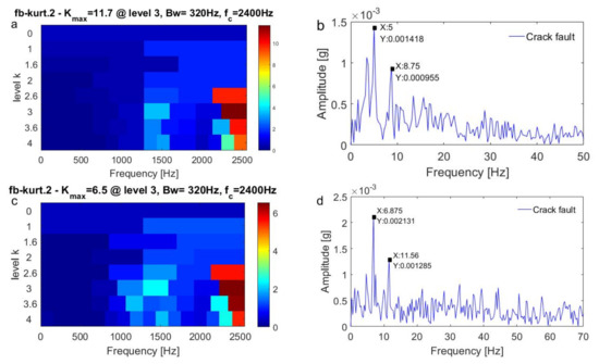
Figure 25.
Fast Kurtogram under(a) 500 rpm, (c) 700 rpm working conditions and the corresponding demodulation spectra under (b) 500 rpm, (d) 700 rpm working conditions.
Based on the enhanced Kurtogram method, the performance of the demodulation spectrum under two conditions was analyzed. As shown in Figure 26, the optimum demodulation scale selected by the enhanced Kurtogram method under both conditions was at (4,8) nodes of the wavelet decomposition, and the frequency range was 1280–1440Hz, as shown in Figure 26a,c respectively. The corresponding demodulation spectra under the two conditions are shown in Figure 26b,d. At 500 rpm, the characteristic frequency of the gear crack fault was found to be 5 Hz. However, compared with the impulse demodulation spectra, the envelope spectra contained a large amount of noise. At 700 rpm, the characteristic frequency of the gear crack fault was 6.875 Hz, but compared with the impulse demodulation spectrum, the envelope spectrum also contained a large number of noise interference components.
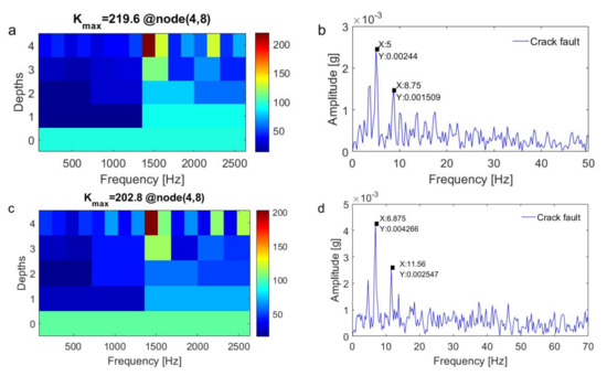
Figure 26.
Enhanced Kurtogram under (a) 500 rpm, (c) 700 rpm working conditions and the corresponding demodulation spectra under (b) 500 rpm, (d) 700 rpm working conditions.
The demodulation spectrum calculated based on the traditional envelope demodulation analysis method is shown in Figure 27. Under the 500 rpm operating condition, a frequency band near six times the meshing frequency of the gearbox was selected for filtering and modulation analysis according to experience. Specifically, the dominant frequency of the spectrum was 680 Hz to 780 Hz. The characteristic frequency of the tooth root crack could not be found in the envelope demodulation spectrum, which contained a large amount of noise, as shown in Figure 27a. Under the 700 rpm operating condition, a frequency band near three times the meshing frequency of the gearbox was selected for filtering and demodulation analysis according to experience. Specifically, the dominant frequency of the spectrum was 470 Hz to 570 Hz. In the envelope demodulation spectrum, frequencies of two times and three times the characteristic frequency of the tooth root crack fault are found, but a large amount of noise was included compared with the impact demodulation spectrum of the proposed method, as shown in Figure 27b.
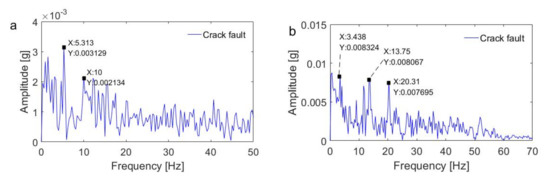
Figure 27.
Envelope spectra calculated from a fixed scale in two working conditions: (a) 500 rpm, (b) 700 rpm.
The values calculated based on the four demodulation methods varied with speed, as shown in Figure 28. It can be seen that the time–frequency multi-scale envelope demodulation always performed well and was superior to the other three methods. The value of the method proposed in this chapter was 19.86 dB higher than that of the fast spectral kurtosis plot method, 16.78 dB higher than that of the enhanced spectral kurtosis plot method and 17.00 dB higher than that of the traditional envelope demodulation method.
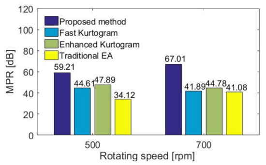
Figure 28.
values of the four methods with different rotating speeds.
In conclusion, the time–frequency multi-scale envelope demodulation algorithm proposed in this work can accurately extract the modulation components caused by faults during the increase and decrease of speed of a fixed-axle gearbox. The fault feature modulation components extracted by the fast spectral kurtosis method at 500 rpm and 700 rpm are heavily contaminated by noise. The modulation components of fault features extracted by the enhanced spectral kurtosis method are more obvious than those obtained by the fast spectral kurtosis method, but they are heavily contaminated by noise compared with the time–frequency multi-scale envelope demodulation algorithm. Traditional envelope demodulation methods cannot adapt to the change of spectrum structure caused by the change of rotational speed, and there are also obvious noise components in the demodulation spectrum.
6. Conclusions
This paper proposed a multi-scale demodulation analysis for the fault diagnosis of a gearbox using a weighted-EMD de-noising technique and time–frequency impulse envelope analysis. Firstly, the modulation mode of a gearbox with a local fault was studied based on a 6 DOF dynamic model, and multi-scale modulation phenomena were found under different rotating speed conditions. Therefore, in this study, we proposed a new TF impulse envelope analysis method of the vibration signal based on continuous wavelet transformation, which allowed the fault-related impulse envelope components in the entire frequency range scale to be extracted. In order to remove the noise components and interference components and improve the quality of the extracted impulse envelope, a weighted-EMD de-noising technique was presented that partitioned the decomposed IMFs to noise-free IMFs or noise-dominant IMFs based on Pearson’s correlation analysis and suppressed the noise using a weighted method. Finally, the proposed method was validated by the fault diagnosis of a planetary gearbox with a sun gear spalling fault and a fixed shaft gearbox with a crack fault, and three usually used methods were adopted for comparison. The demodulation results show that the proposed method could effectively detect both a spalling fault and a crack fault in all data sets and yielded better performance than the fast Kurtogram method, the enhanced Kurtogram method and the traditional envelope analysis method in terms of the ratio.
Author Contributions
Writing—original draft, W.-t.D.; conceptualization, Y.-m.S. and L.-m.W.; methodology, L.-m.W.; validation, Q.Z.; visualization, X.-x.D. All authors have read and agreed to the published version of the manuscript.
Funding
This research received the National Natural Science Foundation of China (Grant No. 51905053, 51805051), the China Postdoctoral Science Foundation (Grant No. 2019M653335) and the Chongqing Postdoctoral Science Foundation (Grant No. cstc2019jcyj-bshX0119) grants.
Conflicts of Interest
The authors declare no conflict of interest.
References
- Guo, Y.; Parker, R.G. Analytical determination of mesh phase relations in general compound planetary gears. Mech. Mach. Theory 2011, 46, 1869–1887. [Google Scholar] [CrossRef]
- Wang, L.; Shao, Y. Fault feature extraction of rotating machinery using a reweighted complete ensemble empirical mode decomposition with adaptive noise and demodulation analysis. Mech. Syst. Signal Process. 2020, 138, 20. [Google Scholar] [CrossRef]
- Chen, Z.; Zhang, J.; Zhai, W.; Wang, Y.; Liu, J. Improved analytical methods for calculation of gear tooth fillet-foundation stiffness with tooth root crack. Eng. Fail. Anal. 2017, 82, 72–81. [Google Scholar] [CrossRef]
- Zhao, M.; Kang, M.; Tang, B.; Pecht, M. Multiple Wavelet Coefficients Fusion in Deep Residual Networks for Fault Diagnosis. IEEE Trans. Ind. Electron. 2019, 66, 4696–4706. [Google Scholar] [CrossRef]
- Huo, Z.; Zhang, Y.; Francq, P.; Shu, L.; Huang, J. Incipient fault diagnosis of roller bearing using optimized wavelet transform based multi-speed vibration signatures. IEEE Access 2017, 5, 19442–19456. [Google Scholar] [CrossRef]
- Ma, R.; Chen, Y. Research on the dynamic mechanism of the gear system with local crack and spalling failure. Eng. Fail. Anal. 2012, 26, 12–20. [Google Scholar] [CrossRef]
- Wang, L.; Shao, Y. Fault mode analysis and detection for gear tooth crack during its propagating process based on dynamic simulation method. Eng. Fail. Anal. 2017, 71, 166–178. [Google Scholar] [CrossRef]
- Chaari, F.; Baccar, W.; Abbes, M.S.; Haddar, M. Effect of spalling or tooth breakage on gearmesh stiffness and dynamic response of a one-stage spur gear transmission. Eur. J. Mech. A Solids 2008, 27, 691–705. [Google Scholar] [CrossRef]
- Kang, M.; Kim, J.; Wills, L.M.; Kim, J.M. Time-varying and multiresolution envelope analysis and discriminative feature analysis for bearing fault diagnosis. IEEE Trans. Ind. Electron. 2015, 62, 7749–7761. [Google Scholar] [CrossRef]
- Rubini, R.; Meneghetti, U. Application of the envelope and wavelet transform analyses for the diagnosis of incipient faults in ball bearings. Mech. Syst. Signal Process. 2001, 15, 287–302. [Google Scholar] [CrossRef]
- McFadden, P.D. Detecting fatigue cracks in gears by amplitude and phase demodulation of the meshing vibration. J. Vib. Acoust. 1986, 108, 165–170. [Google Scholar] [CrossRef]
- Wang, W. Early detection of gear tooth cracking using the resonance demodulation technique. Mech. Syst. Signal Process. 2001, 15, 887–903. [Google Scholar] [CrossRef]
- Bediaga, I.; Mendizabal, X.; Arnaiz, A.; Munoa, J. Ball bearing damage detection using traditional signal processing algorithms. IEEE Instrum. Meas. Mag. 2013, 16, 20–25. [Google Scholar] [CrossRef]
- Fan, X.; Zuo, M. Gearbox fault detection using Hilbert and wavelet packet transform. Mech. Syst. Signal Process. 2006, 20, 966–982. [Google Scholar] [CrossRef]
- Ni, X.; Zhao, J.; Hu, Q.; Zhang, X.; Li, H. A new improved Kurtogram and its application to planetary gearbox degradation feature analysis. J. Vibroeng. 2017, 19, 3413–3428. [Google Scholar] [CrossRef]
- Tra, V.; Kim, J.; Khan, S.A.; Kim, J.M. Incipient fault diagnosis in bearings under variable speed conditions using multiresolution analysis and a weighted committee machine. J. Acoust. Soc. Am. 2017, 142, EL35–EL41. [Google Scholar] [CrossRef] [PubMed]
- Antoni, J. Fast computation of the kurtogram for the detection of transient faults. Mech. Syst. Signal Process. 2007, 21, 108–124. [Google Scholar] [CrossRef]
- Zhang, Y.; Randall, R.B. Rolling element bearing fault diagnosis based on the combination of genetic algorithms and fast kurtogram. Mech. Syst. Signal Process. 2009, 23, 1509–1517. [Google Scholar] [CrossRef]
- Wang, L.; Liu, Z.; Miao, Q.; Zhang, X. Time—Frequency analysis based on ensemble local mean decomposition and fast kurtogram for rotating machinery fault diagnosis. Mech. Syst. Signal Process. 2018, 103, 60–75. [Google Scholar] [CrossRef]
- Lei, Y.; Lin, J.; He, Z.; Zi, Y. Application of an improved kurtogram method for fault diagnosis of rolling element bearings. Mech. Syst. Signal Process. 2011, 25, 1738–1749. [Google Scholar] [CrossRef]
- Wang, D.; Peter, W.T.; Tsui, K.L. An enhanced Kurtogram method for fault diagnosis of rolling element bearings. Mech. Syst. Signal Process. 2013, 35, 176–199. [Google Scholar] [CrossRef]
- Ma, H.; Pang, X.; Feng, R.; Song, R.; Wen, B. Fault features analysis of cracked gear considering the effects of the extended tooth contact. Eng. Fail. Anal. 2015, 48, 105–120. [Google Scholar] [CrossRef]
- Lei, Y.; Kong, D.; Lin, J.; Zuo, M.J. Fault detection of planetary gearboxes using new diagnostic parameters. Meas. Sci. Technol. 2012, 23, 055605. [Google Scholar] [CrossRef]
- Huang, N.E.; Shen, Z.; Long, S.R.; Wu, M.C.; Shih, H.H.; Zheng, Q.; Liu, H.H. The empirical mode decomposition and the Hilbert spectrum for nonlinear and non-stationary time series analysis//Proceedings of the Royal Society of London A: Mathematical, physical and engineering sciences. R. Soc. 1998, 454, 903–995. [Google Scholar] [CrossRef]
- Li, Y.; Xu, M.; Wei, Y.; Huang, W. An improvement emd method based on the optimized rational hermite interpolation approach and its application to gear fault diagnosis. Measuremen 2015, 63, 330–345. [Google Scholar] [CrossRef]
- Yan, R.; Robert, G.; Chen, X. Wavelets for fault diagnosis of rotary machines: A review with applications. Signal Process. 2014, 96, 1–15. [Google Scholar] [CrossRef]
- Singh, A.; Parey, A. Gearbox fault diagnosis under fluctuating load conditions with independent angular re-sampling technique, continuous wavelet transform and multilayer perceptron neural network. IET Sci. Meas. Technol. 2016, 11, 220–225. [Google Scholar] [CrossRef]
- Zhang, X.; He, Y.; Hao, R.; Fulei, C.H.U. Parameters optimization of continuous wavelet transform and its application in acoustic emission signal analysis of rolling bearing. Chin. J. Mech. Eng. 2007, 20, 1. [Google Scholar] [CrossRef]
- Wang, S.; Huang, W.; Zhu, Z. Transient modeling and parameter identification based on wavelet and correlation filtering for rotating machine fault diagnosis. Mech. Syst. Signal Process. 2011, 25, 1299–1320. [Google Scholar] [CrossRef]
- Fyfe, K.R.; Zuo, M.; Lin, J. Mechanical Fault Detection Based on the Wavelet De-Noising Technique. J. Vib. Acoust. 2004, 126, 9–16. [Google Scholar]
- Qiu, H.; Lee, J.; Lin, J.; Yu, G. Wavelet filter-based weak signature detection method and its application on rolling element bearing prognostics. J. Sound Vib. 2006, 289, 1066–1090. [Google Scholar] [CrossRef]
- Wang, H.; Ji, Y. A Revised Hilbert–Huang Transform and Its Application to Fault Diagnosis in a Rotor System. Sensors 2018, 18, 4329. [Google Scholar] [CrossRef]
- Ya, J.; Lu, L. Improved Hilbert–Huang transform based weak signal detection methodology and its application on incipient fault diagnosis and ECG signal analysis. Signal Process. 2014, 98, 74–87. [Google Scholar]
- Lei, Y.; Lin, J.; Zuo, M.J.; He, Z. Condition monitoring and fault diagnosis of planetary gearboxes: A review. Measurement 2014, 48, 292–305. [Google Scholar] [CrossRef]
- Widodo, A.; Kim, E.Y.; Son, J.D.; Yang, B.S.; Tan, A.C.; Gu, D.S.; Mathew, J. Fault diagnosis of low speed bearing based on relevance vector machine and support vector machine. Expert Syst. Appl. 2009, 36, 7252–7261. [Google Scholar] [CrossRef]
Publisher’s Note: MDPI stays neutral with regard to jurisdictional claims in published maps and institutional affiliations. |
© 2020 by the authors. Licensee MDPI, Basel, Switzerland. This article is an open access article distributed under the terms and conditions of the Creative Commons Attribution (CC BY) license (http://creativecommons.org/licenses/by/4.0/).