Fast Fractional-Order Terminal Sliding Mode Control for Seven-Axis Robot Manipulator


Abstract
1. Introduction
- (1)
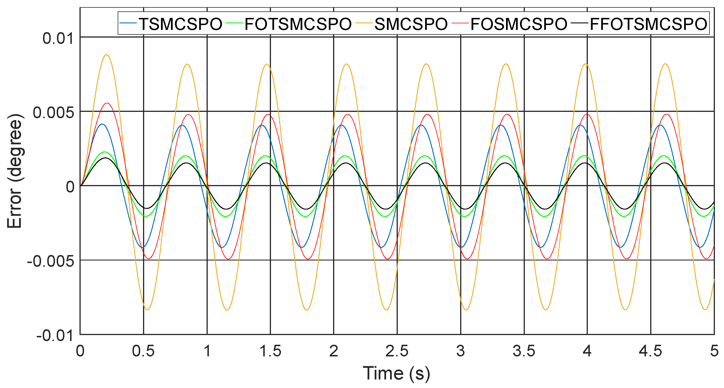
- The new proposed controller, FFOTSMC, uses fractional-order derivatives on both sliding surface design and sliding control/reaching law. It has faster convergence and more outstanding tracking accuracy than FOTSMC, which has been researched previously.
- (2)
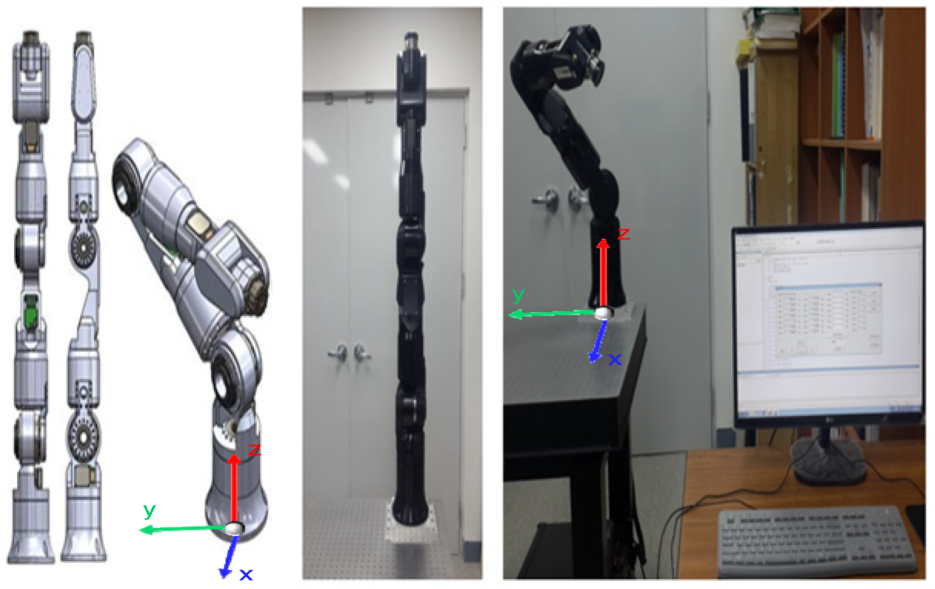
- The new controller FFOTSMC was designed to control a real 7-DOF robot manipulator for trajectory tracking. SPO is used to estimate the disturbance and uncertainties for reducing the chattering, ensuring the controller can be implemented in practice.
- (3)
- Stability is analyzed using the Lyapunov functions for fractional-order systems [16].
2. Preliminaries
2.1. Mathematical Model for Robot Manipulators and Problem Formulation
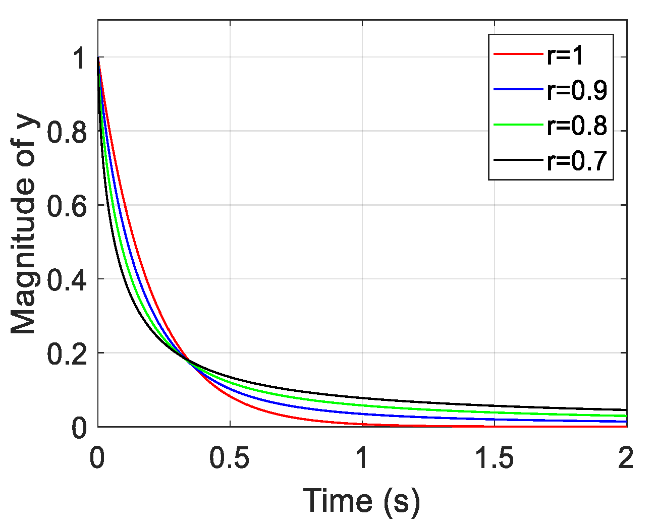
2.2. Fractional Calculus
2.3. Stabilities
3. Controller Design
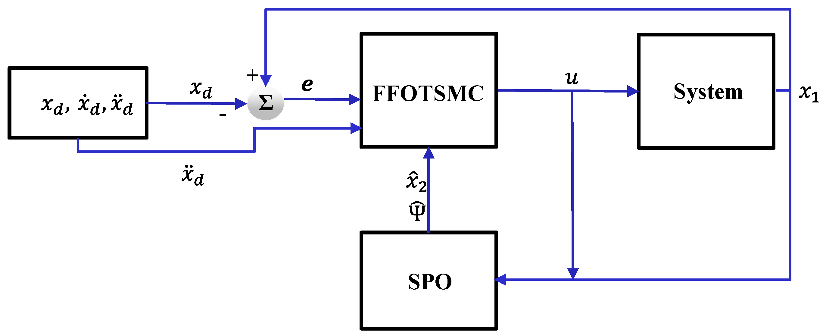
3.1. SPO
3.2. FFOTSMCSPO
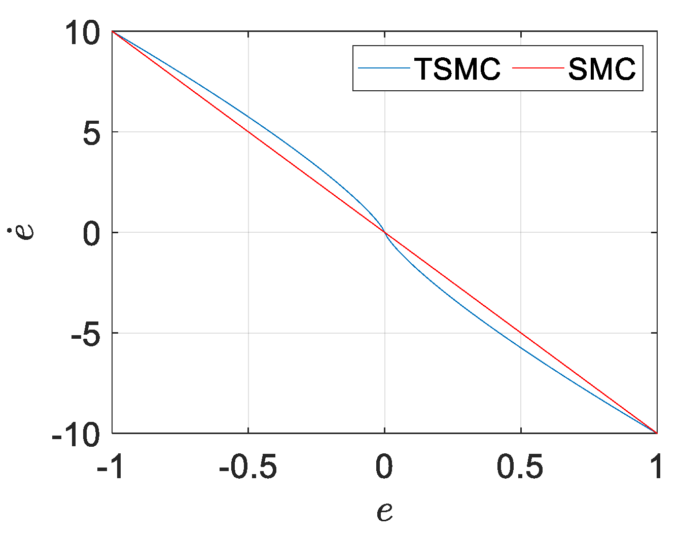
3.2.1. Fractional-Order Sliding Surface
3.2.2. Fast Fractional-Order Sliding Control/Reaching Law
3.3. Stability Analysis
3.4. Numerical Method
4. Simulation and Experiment
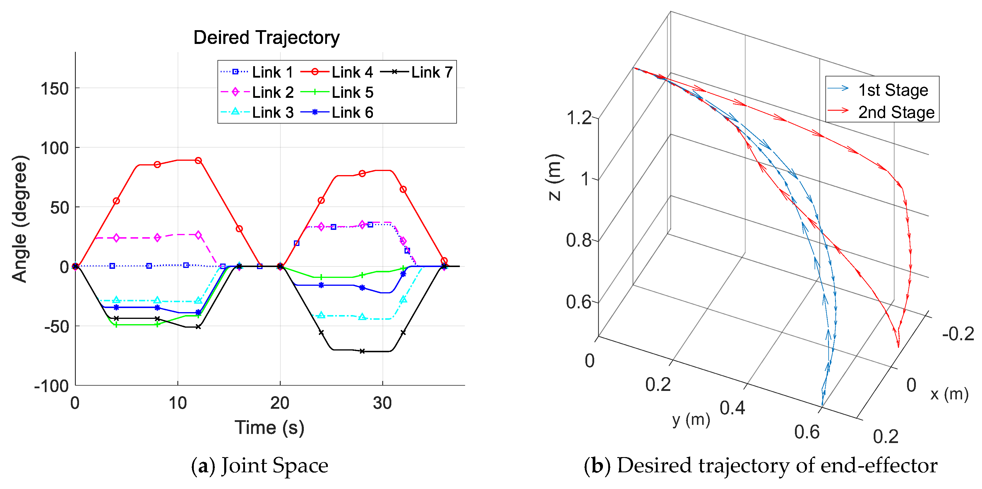
4.1. Simulation
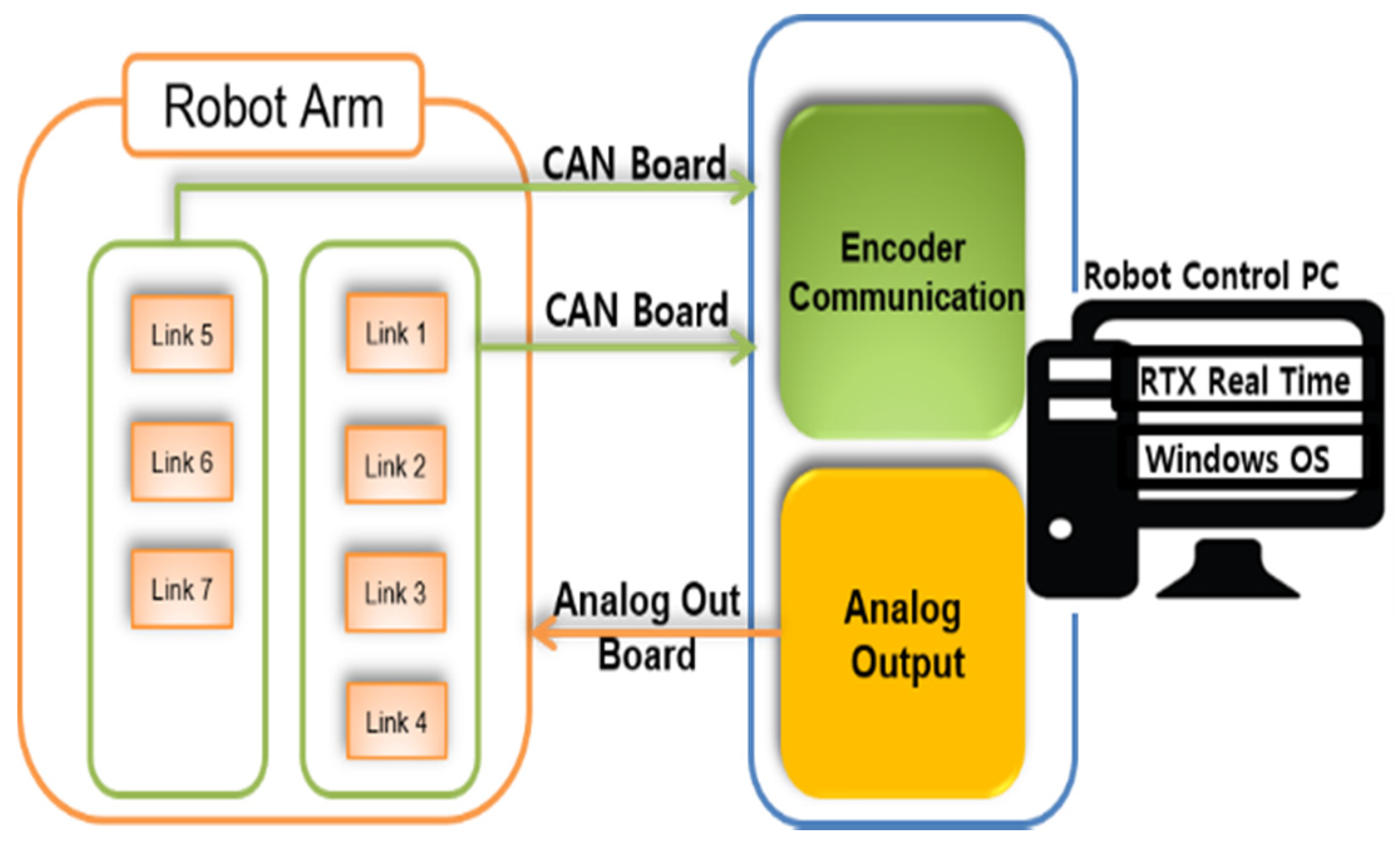
4.2. Experiment
4.2.1. Setting
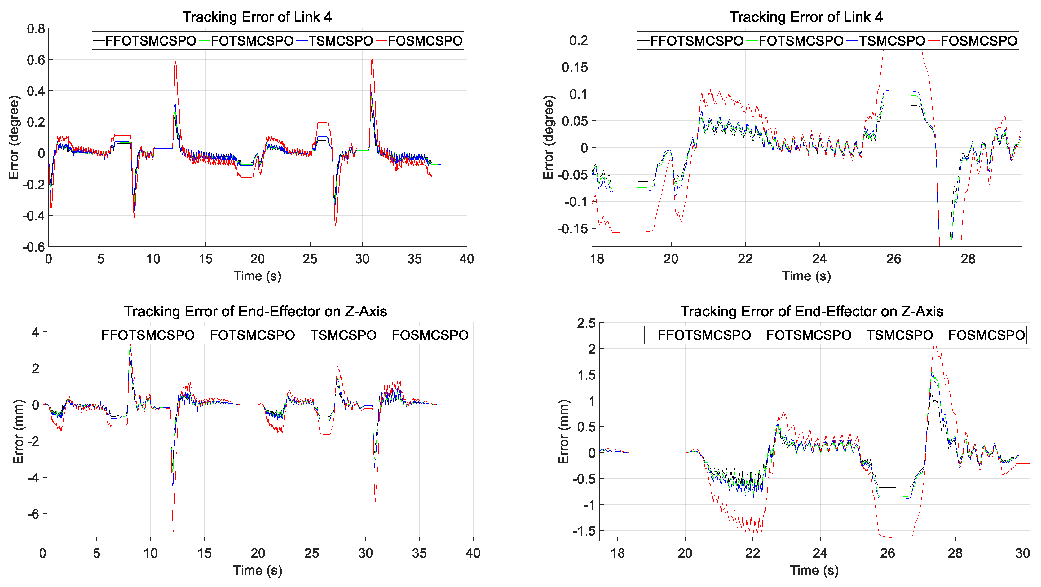
4.2.2. Experimental Results
5. Conclusions
Author Contributions
Funding
Conflicts of Interest
Appendix A


Appendix B
Appendix C

References
- Young, K.D.; Utkin, V.I.; Ozguner, U. A control engineer’s guide to sliding mode control. IEEE Trans. Control. Syst. Technol. 1999, 7, 328–342. [Google Scholar] [CrossRef]
- Zhihong, M.; Yu, X.H. Terminal sliding mode control of MIMO linear systems. In Proceedings of the 35th IEEE Conference on Decision and Control, Kobe, Japan, 13 December 1996; Volume 4, pp. 4619–4624. [Google Scholar]
- Yu, S.; Yu, X.; Shirinzadeh, B.; Man, Z. Continuous finite-time control for robotic manipulators with terminal sliding mode. Automatica 2005, 41, 1957–1964. [Google Scholar] [CrossRef]
- Feng, Y.; Yu, X.; Man, Z. Non-singular terminal sliding mode control of rigid manipulators. Automatica 2002, 38, 2159–2167. [Google Scholar] [CrossRef]
- Feng, Y.; Yu, X.; Han, F. On nonsingular terminal sliding-mode control of nonlinear systems. Automatica 2013, 49, 1715–1722. [Google Scholar] [CrossRef]
- Dadras, S.; Momeni, H.R. Fractional terminal sliding mode control design for a class of dynamical systems with uncertainty. Commun. Nonlinear Sci. Numer. Simul. 2012, 17, 367–377. [Google Scholar] [CrossRef]
- Zhang, B.T.; Pi, Y.G.; Luo, Y. Fractional order sliding-mode control based on parameters auto-tuning for velocity control of permanent magnet synchronous motor. ISA Trans. 2012, 51, 649–656. [Google Scholar] [CrossRef] [PubMed]
- Kilbas, A.A.A.; Srivastava, H.M.; Trujillo, J.J. Theory and Applications of Fractional Differential Equations; Elsevier Science Limited: Amsterdam, The Netherlands, 2006. [Google Scholar]
- Wang, Y.; Luo, G.; Gu, L.; Li, X. Fractional-order nonsingular terminal sliding mode control of hydraulic manipulators using time delay estimation. J. Vib. Control 2016, 22, 3998–4011. [Google Scholar] [CrossRef]
- Sun, G.; Ma, Z.; Yu, J. Discrete-time fractional order terminal sliding mode tracking control for linear motor. IEEE Trans. Ind. Electron. 2017, 65, 3386–3394. [Google Scholar] [CrossRef]
- Wang, Y.; Gu, L.; Xu, Y.; Cao, X. Practical tracking control of robot manipulators with continuous fractional-order nonsingular terminal sliding mode. IEEE Trans. Ind. Electron. 2016, 63, 6194–6204. [Google Scholar] [CrossRef]
- Jie, W.; Yudong, Z.; Bao, Y.; Kim, H.H.; Lee, M.C. Trajectory tracking control using fractional-order terminal sliding mode control with sliding perturbation observer for a 7-DOF robot manipulator. IEEE/ASME Trans. Mechatron. 2020, 25, 1886–1893. [Google Scholar] [CrossRef]
- Moura, J.T.; Elmali, H.; Olgac, N. Sliding mode control with sliding perturbation observer. J. Dyn. Syst. Meas. Control 1997, 119, 657–665. [Google Scholar] [CrossRef]
- Wang, J.; Lee, M.C.; Kallu, K.D.; Abbasi, S.J.; Ahn, S. Trajectory tracking control of a hydraulic system using tsmcspo based on sliding perturbation observer. Appl. Sci. 2019, 9, 1455. [Google Scholar] [CrossRef]
- Lee, M.C.; Kim, C.Y.; Yao, B.; Peine, W.J.; Song, Y.E. Reaction force estimation of surgical robot instrument using perturbation observer with SMCSPO algorithm. In Proceedings of the 2010 IEEE/ASME International Conference on Advanced Intelligent Mechatronics, Montreal, QC, Canada, 6–9 July 2010; pp. 181–186. [Google Scholar]
- Aguila-Camacho, N.; Duarte-Mermoud, M.A.; Gallegos, J.A. Lyapunov functions for fractional order systems. Commun. Nonlinear Sci. Numer. Simul. 2014, 19, 2951–2957. [Google Scholar] [CrossRef]
- Jie, W.; Jamshed, S.; Kim, D.J.; Yulong, B.; Lee, M.C. Trajectory tracking control of a 7-axis robot arm using SMCSPO. In Proceedings of the 2019 International Conference on Intelligent Robotics and Applications, Shenyang, China, 8–11 August 2019; Springer: Cham, Switzerland, 2019; pp. 701–708. [Google Scholar]
- Podlubny, I. Fractional Differential Equations: An Introduction to Fractional Derivatives, Fractional Differential Equations, to Methods of Their Solution and Some of Their Applications; Elsevier: Amsterdam, The Netherlands, 1998. [Google Scholar]
- Li, C.; Qian, D.; Chen, Y. On Riemann–Liouville and caputo derivatives. Discret. Dyn. Nat. Soc. 2011, 2011. [Google Scholar] [CrossRef]
- Deng, W.; Li, C.; Lü, J. Stability analysis of linear fractional differential system with multiple time delays. Nonlinear Dyn. 2007, 48, 409–416. [Google Scholar] [CrossRef]
- Scherer, R.; Kalla, S.L.; Tang, Y.; Huang, J. The Grünwald–Letnikov method for fractional differential equations. Comput. Math. Appl. 2011, 62, 902–917. [Google Scholar] [CrossRef]
- Li, Y.; Chen, Y.Q.; Podlubny, I. Stability of fractional-order nonlinear dynamic systems: Lyapunov direct method and generalized Mittag–Leffler stability. Comput. Math. Appl. 2010, 59, 1810–1821. [Google Scholar] [CrossRef]


| Controller | ||||
|---|---|---|---|---|
| SMCSPO | 1 | 1 | 1 | 1 |
| TSMCSPO | 1 | 1 | 0.9 | 0.9 |
| FOSMCSPO | 1 | 0.7 | 1 | 1 |
| FOTSMCSPO | 1 | 0.7 | 0.9 | 0.9 |
| FFOTSMCSPO | 0.9 | 0.7 | 0.9 | 0.9 |
| Joint | FFOTSMCSPO * | FOTSMCSPO | TSMCSPO | FOSMCSPO | SMCSPO |
|---|---|---|---|---|---|
| 1 | 0.02211 | 0.02430 | 0.02697 | 0.04297 | 0.04837 |
| 2 | 0.01668 | 0.02025 | 0.02178 | 0.04141 | 0.04412 |
| 3 | 0.02347 | 0.02650 | 0.02838 | 0.05033 | 0.05427 |
| 4 | 0.03689 | 0.04238 | 0.04600 | 0.08465 | 0.09360 |
| 5 | 0.06975 | 0.07661 | 0.08230 | 0.11177 | 0.12822 |
| 6 | 0.04323 | 0.04652 | 0.04934 | 0.08188 | 0.08902 |
| 7 | 0.03573 | 0.03634 | 0.04380 | 0.05619 | 0.06348 |
| X-axis | 0.14354 | 0.16122 | 0.17215 | 0.26177 | 0.29921 |
| Y-axis | 0.31273 | 0.36022 | 0.39767 | 0.77066 | 0.86858 |
| Z-axis | 0.26544 | 0.31577 | 0.34160 | 0.60392 | 0.66034 |
Publisher’s Note: MDPI stays neutral with regard to jurisdictional claims in published maps and institutional affiliations. |
© 2020 by the authors. Licensee MDPI, Basel, Switzerland. This article is an open access article distributed under the terms and conditions of the Creative Commons Attribution (CC BY) license (http://creativecommons.org/licenses/by/4.0/).
Share and Cite
Wang, J.; Lee, M.C.; Kim, J.H.; Kim, H.H. Fast Fractional-Order Terminal Sliding Mode Control for Seven-Axis Robot Manipulator. Appl. Sci. 2020, 10, 7757. https://doi.org/10.3390/app10217757
Wang J, Lee MC, Kim JH, Kim HH. Fast Fractional-Order Terminal Sliding Mode Control for Seven-Axis Robot Manipulator. Applied Sciences. 2020; 10(21):7757. https://doi.org/10.3390/app10217757
Chicago/Turabian StyleWang, Jie, Min Cheol Lee, Jae Hyung Kim, and Hyun Hee Kim. 2020. "Fast Fractional-Order Terminal Sliding Mode Control for Seven-Axis Robot Manipulator" Applied Sciences 10, no. 21: 7757. https://doi.org/10.3390/app10217757
APA StyleWang, J., Lee, M. C., Kim, J. H., & Kim, H. H. (2020). Fast Fractional-Order Terminal Sliding Mode Control for Seven-Axis Robot Manipulator. Applied Sciences, 10(21), 7757. https://doi.org/10.3390/app10217757