Abstract
Global Navigation Satellite System (GNSS) can be applied for the navigation of the high-orbit satellites. The system observability will change due to the changes in the visible satellite numbers and the spatial geometry between the navigation satellites and the users in the navigation system. The influence of the observability changing is not considered in the traditional navigation filter algorithm. In this paper, an optimized navigation filter method based on observability analysis is proposed. Firstly, a novel criterion for the relative observable degree is proposed for each observation component by making use of observation data from previous and posterior time simultaneously. Secondly, according to the relationship between observability and navigation filter accuracy, a novel optimized navigation filter method is constructed by introducing an adjusting factor based on the relative observable degree. Through the comparative simulations with the traditional Extended Kalman Filter (EKF), the optimized navigation filter method can reduce the estimation error of position and velocity by about 36% and 44% respectively. Therefore, the superiority of the proposed filter optimization algorithm is verified.
1. Introduction
High-orbit satellites [1] have better performance for ground coverage, safety, and stability compared with low-orbit and medium-orbit ones. For this reason, they play an important role in practice, e.g., satellite navigation and positioning systems. GNSS is the general term for all satellite navigation and positioning systems in orbit [2,3]. The position and velocity estimation of the users can be obtained based on GNSS by measuring the pseudo-range and Doppler frequency shift between the users and the navigation satellites. It has the advantages of comprehensive navigation information, high navigation accuracy, and simple measurement equipment [4], and has been widely applied in reality [5,6,7,8,9,10]. The navigation of the high-orbit satellites based on GNSS is one of the important research areas in the high-orbit satellite navigation technology.
The observability is the premise and the foundation of the navigation system with good navigation performance. The concept of observability was firstly proposed by Kalman [11], which refers to the ability of the navigation system to estimate the state variables through the outputs or the observations of the navigation system. In the engineering practice, we consider that the observability can be extended to the following three levels: the geometric observability, the physical observability, and the engineering observability. For the navigation system of high-orbit satellites based on GNSS, the geometrical observability refers to that the line of sight of the high-orbit satellite to the navigation constellation is visible, the physical observability refers to that the effective observation data of the high-orbit satellite measurement equipment on the GNSS navigation satellite can be obtained and the engineering observability refers to that after obtaining effective observation data, the value of the user’s state variables that meet the engineering accuracy requirements can be estimated. These three levels of observability are names as ’visibility’, ’testability’, and ’availability’. Among them, the ’availability’ in this article refers to the observability in the control field. It is the basis for judging the performance of the navigation system and the reflection of the ability of the control system to determine the state variables at the initial moment [12]. In addition, good observability is the guarantee for the state filter convergence of the navigation system of high-orbit satellite [13,14]. Therefore, research on the observability of the navigation system is an important link in the design of the navigation system and the optimization of the navigation filter algorithm and has important theoretical and practical significance.
Since the navigation system of high-orbit satellites based on GNSS is a nonlinear system, there are currently two main methods to analyze the observability for the nonlinear system: one is to transfer the nonlinear system into a linear system by linearizing the nonlinear system and then distinguish the observability by using the Grammar matrix of the linear system [15,16]. The second method analyzes the observability of the navigation system through the observability discriminant matrix which can be computed through the Lie derivative in the differential manifold [17,18]. However, the calculation complexity of the second method is high and its operating efficiency may also be reduced when the system equation is complex. The observability can only qualitatively judge whether the navigation system is observable. To quantify the observability of the system and its state components, the observable degree needs to be applied [19]. The analysis method of the observable degree has not been clearly defined. Ham [20] firstly proposed the method in 1983 which uses the eigenvalues and eigenvectors of the estimated error covariance matrix to describe the observability of the system state. However, the method can only work after the filter, and the system observability cannot be given in real-time. Reference [21] proposed a method to analyze the observable degree of the system through the singular value of the observable matrix. The method can judge the observability of the system before filter and is a pre-analysis method. However, this method can only give the overall observability of the system and cannot obtain the observability for each state component of the system. Reference [22] defined a method which analyzes the observable degree according to the error attenuation degree of the initial state variables, but the method paid much attention to the initial error covariance and ignored the real-time performance of filter; besides, some studies proposed to use the Fisher information matrix are also used to measure the observability of the navigation system in some studies [23,24,25].
Currently, there are many navigation filter algorithms applied to the navigation systems of the high-orbit satellites, including traditional Kalman filter and various improved forms. In addition, many scholars have proposed a large number of corresponding improved filter algorithms for the nonlinearity and uncertainty of the actual navigation system as well as the non-gaussian and correlation of noise, etc. [26,27,28,29,30]. Reference [31] proposed an adaptive filter method based on the state observability. The method constructed some adaptive factors according to the proposed quantized observability of each state component. The filter gain attenuation method is simultaneously applied to adjust the components whose observability is weak. Reference [32] proposed an information fusion algorithm based on the observable degree. The algorithm determines the information distribution coefficient according to the observable degree of the observation model and takes the unscented filter as the federated filter algorithm. Reference [33] proposed a smart Kalman filter method based on the adaptive observability to solve the problem of inaccurate parameters of the observation equation. The method improves the filter robustness by iteratively solving the adaptive adjustment factor.
However, the observable degree of the different state variables of the navigation system is inconsistent and the information transmitted to the subsequent filter estimation is also inconsistent. The previous research mainly used the observability directly as an adjustment factor and fed it back to the filter to improve the importance of the state variables with strong observability, while to reduce the influence of state variables with weak observability. Since the observability results obtained by different observability measurement methods are not consistent, it may cause the navigation filter divergence and reduce the overall navigation performance. In addition, the high-orbit satellite navigation is different from the general navigation system because the high-orbit satellite is higher than most orbits of the four major satellite navigation systems at present. Superadd the transmitting antenna of the GNSS satellite is facing the earth [34], and the angle between the main lobe signal transmission is limited. When the high-orbit satellite moves beyond the GNSS constellation, it can only receive the navigation satellite signal from the other side of the earth [35]. Therefore, the number of navigation satellites (i.e. the number of the visible satellites) that can be observed by the satellite at the receiver antenna position is limited. In a cycle of satellite operation, the number of visible navigation satellites changes constantly, which leads to the change of the observability. Therefore, it is of great significance to optimize the existing navigation filter algorithm and improve the overall performance of the navigation system of high-orbit satellites based on GNSS with the observability and the observable degree of the navigation system.
Based on the above analysis, we propose an adaptive navigation filter optimization method based on the observability and the observable degree of local components. According to the attenuation degree between the error of the optimal solution obtained from the observation in a period and the error of the state variable estimated by the filter at the current time, a new observability calculation matrix is defined, and the relative observable degree of each state component of the system is obtained. The advantages of this optimization method are that it can improve the traditional navigation filter method which only uses the observation information of the previous time, and can adjust the original filter process with the feedback of the observation information during the later time and the degree of error attenuation, which effectively improves the navigation filter accuracy and reduces the estimation error. The main contributions of this paper are as follows:
- (1)
- We propose a new method for calculating the observable degree of a high-orbit satellite navigation system based on GNSS, which can simultaneously give the relative observability of each state component at each moment and the overall observability of the system;
- (2)
- We design an adaptive optimization method of navigation filter based on this observable degree, which maps the observable degree of the state component to a feedback weighting factor to improve the performance of the navigation filter;
- (3)
- Based on the GNSS navigation system, we combine the proposed observability calculation method as an adjustment factor of the adaptive filter for filter optimization. Numerical simulation shows that the method effectively improves the navigation filter accuracy of the navigation systems of the high-orbit satellite based on GNSS.
The rest of this article is organized as follows. In Section 2, we briefly introduce the state equation and measurement equation of the high-orbit satellite navigation system based on GNSS. In Section 3, we analyze the observability of the system and propose the observability matrix of the system. Furthermore, the observable degree calculation matrix of the system is defined. In Section 4, according to the proposed framework for the observable degree, we propose an adaptive filter method. In Section 5, we verify the effectiveness of the proposed method by simulation of the high-orbit satellite navigation system based on GNSS. Section 6 is the summary and prospect of the full text.
4. Optimized Filter Algorithm for Navigation System Based on the Observable Degree
As the observability is related to the filter accuracy tightly, one of the most efficient methods to increase the accuracy is to optimize the filter algorithm based on the observability. In this paper, a novel Adaptive extend Kalman Filter (AKF) base on the novel observability criterion is proposed for the navigation system of high-orbit satellites. The framework is summarized in Figure 1. The details of the method will be reported in the following part.
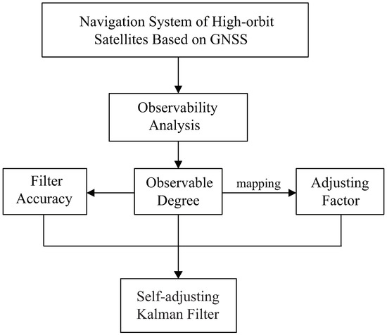
Figure 1.
The framework of navigation filter optimization algorithm proposed in the paper.
The traditional process of EKF is reported as follows.
The one-step prediction of the state vector is
The error covariance matrix of is
The filter gain matrix is
The prediction of state vector is
The error covariance matrix of is
Recent works contribute a variety of the frameworks of the adaptive Kalman Filter, in the paper, we choose the framework with an adjusting factor in front of the filter gain in Equation (21). Then the adaptive filter gain matrix can be written as
where is a diagonal matrix. The value of the i-th diagonal element of is the adjusting factor of the corresponding i-th state variable.
Increasing the value of the adaptive adjustment factor will change the value of the original gain matrix which can be considered as a balance parameter between the one-step predicted value of the state variable and the observed value. When the navigation system suffers a weak observable degree, in order to suppress the influence of the weak observable degree, adjusting the weighting method can be used to correct the bias of predicted state variables.
As we discussed above, the observability plays an important role in the navigation system. The adjusting factor should also be designed for each state variable in order to suppress the influence of weak observable degree. This conclusion is obviously correct because if we use an identical factor for all the state variables, the effect of the adjusting factor will modify the state variables at an equal level. The state variable with a high observable degree will be incorrect and the filter accuracy will be decreased.
In the previous section, we have proposed a relative observable degree for each state variable. Meanwhile, the prediction of each state variable is closely related to the observable degree. For this reason, a criterion for defining the adaptive adjusting factor based on the relative observable degree is proposed.
The definition of can be expressed as
where the subscript represents the i-th diagonal element and which donates the observable degree in k-th moment is defined in Equation (18). is a mapping function which represents the relationship between the observable degree and the adjusting factor.
In the adjusting process, since the original state estimations are biased under weak observable degree, in order to reduce the bias, the adjusting factor should be well designed. For example, when the observation component has a high observable degree, the estimation should rely more on the observation information. In opposite, the estimation should rely more on state prediction.
Based on the navigation system in this paper, the observation Equation (3) shows that
where is the position vector of the high-orbit satellites. This Equation (26) indicates that the state observation is related to the position vector immediately and has little relationship with the velocity vector. Hence, the setting of the adjusting factor should consider the position vector and the velocity vector respectively. For the position vector, as the observable degree is a kind of relative value, the component with the best observable degree should hold the original estimation and its adjusting factor should be 1. When the state is ideal, if we notate the error of as , then the optimal filter gain is the solution of
However, when suffering a weak observable degree, the estimation error has a larger variance. An inequality can be derived that
Compared with Equations (29) and (30), we can find that when the observable degree is weak, the is larger than . Hence, in order to reduce the error covariance, the adjusting factor should be larger than 1.
Based on the analysis above, we can optimize the EKF through the adjusting factor. Theprocess of our Algorithm 1 can be expressed as follows
| Algorithm 1 Adaptive Extend Kalman Filter |
| 1: Input: Optimal estimation of and covariance matrix in moment |
| 2: Output: Optimal estimation of and covariance matrix in moment k |
| Step 1: Calculate the state transition , measurement matrix and state covariance matrix by Equations (19)–(23) |
| Step 2: Repeat Step 1 and calculate the state transition matrix and measurement matrix at moment , written as . |
| Step 3: Use the in Step 1 and Step 2 then calculate the by Equation (18). |
| Step 4: Define a mapping function based on the criterion in Section 3 then calculate the by Equation (25). |
| Step 5: Calculate the new filter gain matrix by Equation (24). |
| Step 6: Calculate and and output them. |
5. Simulation Analysis
In this section, we take the navigation system of high-orbit satellites based on GNSS in the high-orbit environment as the simulation background and use the observability theory and navigation filter optimization as the research methods to simulate and analyze the EKF and the navigation filter optimization method proposed in this paper.
5.1. Simulation Conditions
In this paper, we assume that the navigation system is the Beidou satellite navigation system. The initial epoch is UTC 0h0min0s on 28 May 2020. The Beidou navigation satellite orbit simulation data is obtained from the TLE data by the North American Aerospace Defence Command. Figure 2 is an illustration of the orbits of three BEIDOU navigation systems (contains BDS-1, BDS-2, BDS-3) including 49 satellites, and these orbits are represented by different colors. An inclined geo-synchronization orbit (IGSO) satellite is the user satellite. The coordinate system used in the simulation is the J2000.0 geocentric inertial coordinate system, the time system is Coordinated Universal Time (UTC). The simulation duration is 43080 s, and the sampling time interval is 4 s. In the experiment, only the main lobe signal of the navigation satellite has been considered, and the receiver sensitivity has not been considered. Set the half-angle of the main lobe signal beam as , and the half-angle of the part occluded by the earth as . The satellite orbit dynamics model of user satellite is set as a two-body model, with a mean square error of position error of 10 m and a mean square error of velocity error of 0.1 m/s [39,40], the mean square error of measured white noise is set to be 1 m, and the position and velocity at the initial moment are
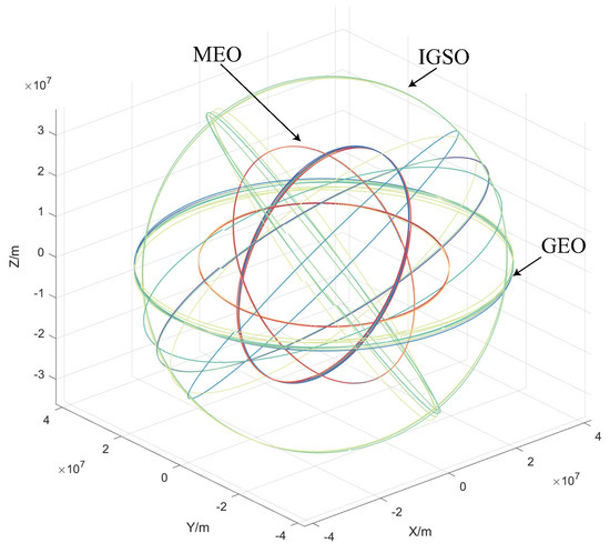
Figure 2.
This is the Beidou navigation constellation map under J2000.0 geocentric inertial coordinate system.
The error covariance matrix at the initial moment is
According to Section 3.2, due to the real-time requirements of the navigation system of high-orbit satellites, in the observability calculation matrix, the parameter m equals to 1. According to the selection criteria of the adjustment factor in Section 4, if the number of visible satellites is larger than 3, the observability mapping function is constructed as
If the number of visible satellites is smaller than 3,
5.2. Simulation Results and Analysis
First, we obtain the number of the visible satellites at different times according to the geometric relationship between the navigation satellites and the user satellites, which is shown in Figure 3a. From the observability analysis of the system in Section 3.1, the rank of the observability discriminant matrix during the entire sampling duration is calculated to be 6 all the time, which shows that the system is observable during the entire simulation process. Then the condition number is calculated. The condition number of the observable matrix during the simulation process is shown in Figure 3b. According to the observability calculation formula in Section 3.2, the observable degree of each state component of the system is obtained. Figure 4a shows the observable degree of the position vector at different moments, and Figure 4b shows the observable degree of the velocity vector at different moments. In this paper, EKF and the improved adaptive filter are used to evaluate the overall system and each state variable. Figure 5 shows the average error of each state component in the corresponding sampling period. The filter results obtained are shown in Figure 6. Figure 6 reflects the comparison result between the residual error of EKF and adaptive filter estimation results for each state variable. Figure 7a,b reflect the comparison result between diagrams of EKF and adaptive filter position estimation error and velocity estimation error respectively. Figure 8a,b are the comparison figures of the filter position and velocity error of the period with high observability respectively. Taking 8000–10,000 sampling points as an example, Figure 9 shows the comparison result between the observability of the state variable component y and its residual error result.
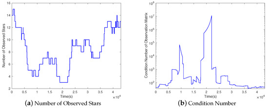
Figure 3.
Figure (a) is the figure of number of observed stars. The abscissa is sampling time. Figure (b) is the figure of condition number of observation matrix. The abscissa is sampling time. The abscissas in follow figures are the same.
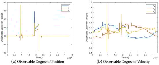
Figure 4.
(a,b) show the observable degree of position and velocity respectively. The abscissa is sampling time.
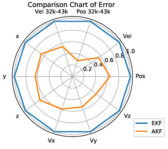
Figure 5.
The radar figure shows the rate between estimation errors of EKF and AKF. The evaluation criterion is the mean error. The ’x’,’y’,’z’,’Vx’,’Vy’,’Vz’ represent the each state variable respectively. The ’Pos’,’Vel’ represent the position and velocity respectively. The ’Pos 32k-43k’,’Vel 32k-43k’ represent the position and velocity during 32,000 s–43,080 s respectively.
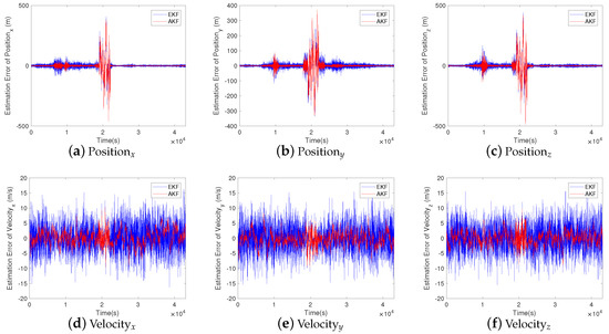
Figure 6.
The figure reflects estimation error of each state variable between EKF and AKF.
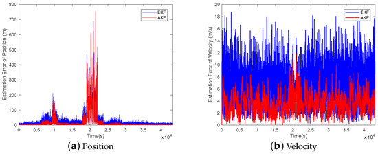
Figure 7.
The figure reflects estimation error of position and velocity by EKF and AKF.
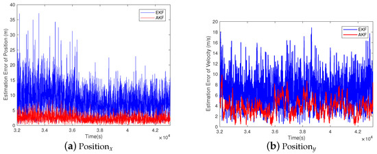
Figure 8.
The figure reflects estimation error of position and velocity by EKF and AKF in period between 32,000 s and 43,080 s.
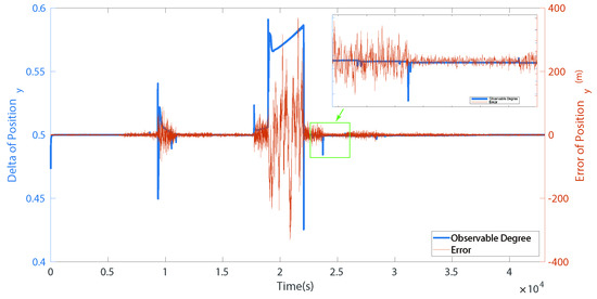
Figure 9.
This is a comparison chart between error and observable degree at portion y.
According to the simulation experiment results above, this paper mainly analyzes from the following aspects:
(1) The results of the high-orbit satellite navigation are directly related to the number of the visible satellites and changes in observability. From Figure 3a,b and Figure 4, it can be seen that the number of the visible satellites changes constantly in the simulation period. When the number decreases, the observability matrix condition number becomes larger, and the observability of the position of each state component becomes weaker, the filter estimation error also becomes larger. When the number of the visible satellites increases, the condition number of the observability matrix becomes smaller, and the observability of the position state component becomes stronger and the filter estimation has lower error.
(2) The accuracy of the adaptive filter based on observability has been significantly improved compared with conventional methods. It can be seen from Figure 5, Figure 6, Figure 7, Figure 8 and Figure 9 that in the entire navigation process, the optimized navigation filter method can reduce the estimation error of position and velocity by about 36% and 44% respectively compared with the original EKF, which verifies the effectiveness of this method proposed in this article. It can be seen from Figure 8 that in the period when the number of visible satellites is large, the adaptive filter method will reduce the position error more significantly, and the result is reduced by nearly 70%. This shows that when there exist enough visible satellites, the observability of the overall state variable will be strong, and the proposed navigation filter optimization method will achieve better performance than the other cases.
(3) The observability calculation method for state components proposed in this paper can reflect the changes in the filter accuracy of each component. It can be seen from Figure 9 that the observable degree of the state component y becomes smaller, its observability becomes relatively better, and the residual error in the y direction also rapidly becomes smaller. This result further verifies the relationship between observability and filter accuracy. When the observability is strong, the filter accuracy of the state variable is high.
6. Conclusions
To address the problem of the variable number of the visible satellites of the satellite navigation system in a high-orbit environment, this paper discusses the observability of the navigation system and proposes an adaptive navigation filtering optimization method based on the observability analysis. Firstly, the observability of the navigation system is analyzed, and a novel observability calculation method is proposed based on minimizing the objective function of error loss. Then the observable degree of different state variables can be derived. Secondly, according to the relationship between the observability and the filtering accuracy, a mapping value of the observable is applied as the feedback adjustment coefficient to construct an adaptive filter method. This method can combine the information of the previous period and the next period simultaneously to obtain feedback on the filter process. Through this approach, the estimation error can be effectively reduced. Simulation experiments on the high-orbit satellites of the Beidou navigation system show that the proposed adaptive EKF achieves better performance compared with traditional EKF, and verify the effectiveness and practicability of the novel method.
In order to further improve the navigation accuracy, the next main work will focus on the effective method of combining observability with other filter methods, and combining the optimization methods to improve the filter accuracy.
Author Contributions
Q.X. proposed the main idea, finished the draft manuscript; X.Z. and J.W. conceived of the experiments and drew the figures and tables; Methodology, Y.X.; Z.H. analyzed the data; H.Z. conducted the simulations. All authors have read and agreed to the published version of the manuscript.
Funding
This research was funded by the National Natural Science Foundation of China [grant number 61773021, 61903086 and 61903366], the National Natural Science Foundation of Hunan Province [grant number 2019JJ20018, 2019JJ50745 and 2020JJ4280], Department of Education of Guangdong Province [grant number 2019KTSCX193] and Fundamentals and Basic of Application Research Foundation of Guangdong Province [grant number 2019A1515110136].
Conflicts of Interest
The authors declare no conflict of interest.
Abbreviations
The following abbreviations are used in this manuscript:
| GNSS | Global Navigation Satellite System |
| EKF | Extend Kalman filter |
| AKF | adaptive Kalman filter |
| IGSO | inclined geo-synchronization orbit |
| UTC | Universal Time |
References
- Chory, M.A.; Hoffman, D.P.; Lemay, J.L. Satellite autonomous navigation—Status and history. In Office of Entific & Technical Information Technical Reports; Institute of Electrical and Electronics Engineers: New York, NY, USA, 1986; pp. 110–121. [Google Scholar]
- Moreau, M.C.; Axelrad, P.; Garrison, J.L.; Kelbel, D.; Long, A. GPS Receiver Architecture and Expected Performance for Autonomous Navigation in High Earth Orbits. Navigation 2000, 47, 190–204. [Google Scholar] [CrossRef]
- Rycroft, M.J. Understanding GPS: Principles and Applications. J. Atmos. Sol.-Terr. Phys. 1996, 59, 598–599. [Google Scholar] [CrossRef]
- Gao, W.; Zhang, Y.; Wang, J. A Strapdown Interial Navigation System/Beidou/Doppler Velocity Log Integrated Navigation Algorithm Based on a Cubature Kalman Filter. Sensors 2013, 14, 1511–1527. [Google Scholar] [CrossRef] [PubMed]
- Burdziakowski, P. A Novel Method for the Deblurring of Photogrammetric Images Using Conditional Generative Adversarial Networks. Remote Sens. 2020, 12, 2586. [Google Scholar] [CrossRef]
- Chen, Q.; Zhang, Q.; Niu, X. Estimate the Pitch and Heading Mounting Angles of the IMU for Land Vehicular GNSS/INS Integrated System. IEEE Trans. Intell. Trans. Syst. 2020, 1–13. [Google Scholar] [CrossRef]
- Paziewski, J.; Crespi, M. High-precision multi-constellation GNSS: Methods, selected applications and challenges. Meas. Technol. 2020, 31, 010101. [Google Scholar] [CrossRef]
- Specht, C.; Lewicka, O.; Specht, M.; Dbrowski, P.S.; Burdziakowski, P. Methodology for Carrying Out Measurements of the Tombolo Geomorphic Landform Using Unmanned Aerial and Surface Vehicles near Sopot Pier, Poland. J. Mar. Eng. 2020, 8, 384. [Google Scholar] [CrossRef]
- Specht, C.; Lewicka, O.; Specht, M.; Dbrowski, P.S.; Burdziakowski, P. Road Tests of the Positioning Accuracy of INS/GNSS Systems Based on MEMS Technology for Navigating Railway Vehicles. Energies 2020, 17, 4463. [Google Scholar] [CrossRef]
- Stateczny, A.; Burdziakowski, P.; Najdecka, K.; Domagalska-Stateczna, B. Accuracy of Trajectory Tracking Based on Nonlinear Guidance Logic for Hydrographic Unmanned Surface Vessels. Sensors 2020, 20, 832. [Google Scholar] [CrossRef]
- Kalman, R.E. A New Approach to Linear Filtering and Prediction Problems. J. Basic Eng. 1960, 82, 35–45. [Google Scholar] [CrossRef]
- Ge, Q.; Ma, J.; Chen, S.; Wang, Y.; Bai, L. Observable Degree Analysis to Match Estimation Performance for Wireless Tracking Networks. Asian J. Control 2017, 19, 1259–1270. [Google Scholar] [CrossRef]
- Wang, X.-M.; Cui, H.-T.; Cui, P.-Y. Robustness of observability of linear systems. J. Jilin Univ. (Eng. Technol. Ed.) 2019, 39, 286–290. [Google Scholar]
- Liu, Y.; Cui, P. Observability Analysis of Deep-space Autonomous Navigation System. In Proceedings of the Chinese Control Conference, Harbin, China, 7–11 August 2006. [Google Scholar]
- Bender, E.M.; Flickinger, D.; Oepen, S. The Grammar Matrix: An Open-Source Starter-Kit for the Rapid Development of Cross-Linguistically Consistent Broad-Coverage Precision Grammars. In Proceedings of the 2002 Workshop on Grammar Engineering and Evaluation; Association for Computational Linguistics: Stroudsburg, PA, USA, 2002; Volume 15, pp. 1–7. [Google Scholar]
- Wood, D. Bicolored digraph grammar systems. In Rairo Informatique Theorique et Applications/Theoretical Informatics & Applications; EDP SCIENCES S A: Les Ulis, France, 1973. [Google Scholar]
- Hermann, R.; Krener, A. Nonlinear controllability and observability. IEEE Trans. Automat. Contr. 1977, 22, 728–740. [Google Scholar] [CrossRef]
- Chen, Z. Local observability and its application to multiple measurement estimation. Ind. Electron. IEEE Trans. 1991, 38, 491–496. [Google Scholar] [CrossRef]
- Zhang, L.; Neusypin, K.A.; Selezneva, M.S. A New Method for Determining the Degree of Controllability of State Variables for the LQR Problem Using the Duality Theorem. Appl. Sci. 2020, 10, 5234. [Google Scholar] [CrossRef]
- Ham, F.M.; Brown, R.G. Observability, Eigenvalues, and Kalman Filtering. IEEE Trans. Aerosp. Electron. Syst. 1983, AES-19, 269–273. [Google Scholar] [CrossRef]
- Cheng, X.; Dejun, W. Study on Observability and Its Degree of Strapdown Inertial Navigation System. J. Southeast Univ. 1997, 27, 6–11. [Google Scholar]
- Baram, Y.; Kailath, T. Estimability and Regulability of Linear Systems. IEEE Trans. Autom. Control 1988, 33, 1116–1121. [Google Scholar] [CrossRef]
- Jauffret, C. Observability and fisher information matrix in nonlinear regression. Aerosp. Electron. Syst. IEEE Trans. 2007, 43, 756–759. [Google Scholar] [CrossRef]
- Sun, D.; Crassidis, J.L. Observability Analysis of Six-Degree-of-Freedom Configuration Determination Using Vector Observations. J. Guid. Control Dyn. 2002, 25, 1149–1152. [Google Scholar] [CrossRef]
- Tichavsky, P.; Muravchik, C.H.; Nehorai, A. Posterior Cramer-Rao bounds for discrete-time nonlinear. IEEE Trans. Signal Process. 1998, 46, 1386–1396. [Google Scholar] [CrossRef]
- Xiong, K.; Liu, L. Design of parallel adaptive extended Kalman filter for online estimation of noise covariance. Aircr. Eng. 2019, 91, 112–123. [Google Scholar] [CrossRef]
- Xiong, K.; Wei, C. Adaptive Iterated Extended KALMAN Filter for Relative Spacecraft Attitude and Position Estimation. Asian J. Control 2018, 20, 1595–1610. [Google Scholar] [CrossRef]
- Bermudez, J.; Valdés, R.M.A.; Comendador, V.F.G. Engineering Applications of Adaptive Kalman Filtering Based on Singular Value Decomposition (SVD). Appl. Sci. 2020, 10, 5168. [Google Scholar] [CrossRef]
- Tan, T.N.; Khenchaf, A.; Comblet, F.; Franck, P.; Champeyroux, J.M.; Reichert, O. Robust-Extended Kalman Filter and Long Short-Term Memory Combination to Enhance the Quality of Single Point Positioning. Appl. Sci. 2020, 10, 4335. [Google Scholar] [CrossRef]
- Alammari, A.; Alkahtani, A.; Riduan, M.; Noman, F.; Esa, M.R.M.; Muhammad, H.M.S.; Mohammad, S.A.; Salih Al-Khaleefa, A.; Kawasaki, Z.; Agelidis, V. Kalman Filter and Wavelet Cross-Correlation for VHF Broadband Interferometer Lightning Mapping. Appl. Sci. 2020, 10, 4238. [Google Scholar] [CrossRef]
- Liang, H.; Wang, D.D.; Mu, R.J. Adaptive filtering algorithm based on observable degree analysis of state parameters in carrier-aircraft transfer alignment. Zhongguo Guanxing Jishu Xuebao/J. Chin. Inert. Technol. 2014, 22, 58–62. [Google Scholar]
- Chu, Y.; Wang, D.; Huang, X. Observability Analysis Based Information Fusion Integrated Navigation. Aerosp. Control 2011, 29, 31–41. [Google Scholar]
- Ge, Q.; Ma, J.; He, H.; Li, H.; Zhang, G. A basic smart linear Kalman filter with online performance evaluation based on observable degree. Appl. Math. Comput. 2020, 367, 124603. [Google Scholar] [CrossRef]
- Filippi, H.; Gottzein, E.; Kuehl, C.; Mueller, C.; Barrios-Montalvo, A.; Dauphin, H. Feasibility of GNSS receivers for satellite navigation in GEO and higher altitudes. In Proceedings of the 5th ESA Workshop on Satellite Navigation Technologies and European Workshop on GNSS Signals and Signal Processing (NAVITEC), Noordwijk, The Netherlands, 8–10 December 2010; pp. 1–8. [Google Scholar]
- Dion, A.; Calmettes, V.; Bousquet, M.; Boutillon, E. Performances of a GNSS receiver for space-based applications. arXiv 2018, arXiv:1809.10086. [Google Scholar]
- Qiao, L.; Lim, S.; Liu, J. Autonomous GEO Satellite Navigation with Multiple GNSS Measurements. In Proceedings of the 22nd International Meeting of the Satellite Division of The Institute of Navigation, Savannah, GA, USA, 22–25 September 2009; pp. 2169–2177. [Google Scholar]
- Hong, S.; Chun, H.H.; Kwon, S.H.; Lee, M.H. Observability Measures and Their Application to GPS/INS. IEEE Trans. Veh. Technol. 2008, 57, 97–106. [Google Scholar] [CrossRef]
- Shang, Z.; Ma, X.; Liu, Y.; Ya, S. Adaptive hybrid Kalman filter based on the degree of observability. In Proceedings of the 34th Chinese Control Conference (CCC), Hangzhou, China, 28–30 July 2015. [Google Scholar]
- Park, E.S.; Park, S.Y.; Roh, K.M.; Choi, K.H. Satellite orbit determination using a batch filter based on the unscented transformation. Aerosp. Sci. Technol. 2010, 14, 387–396. [Google Scholar] [CrossRef]
- Qiao, L.; Lim, S.; Rizos, C.; Liu, J. GNSS-Based Orbit Determination for Highly Elliptical Orbit Satellites. Earth 2009, 2, 3. [Google Scholar]


Publisher’s Note: MDPI stays neutral with regard to jurisdictional claims in published maps and institutional affiliations. |
© 2020 by the authors. Licensee MDPI, Basel, Switzerland. This article is an open access article distributed under the terms and conditions of the Creative Commons Attribution (CC BY) license (http://creativecommons.org/licenses/by/4.0/).