Abstract
The transient proper orthogonal decomposition (TPOD) method is applied for order reduction in the rotor-bearing system with the coupling faults in this paper. A 24 degrees of freedom (DOFs) rotor model supported by a pair of sliding bearings with both crack and rub-impact faults is established by the discrete modeling method. The complexity of dynamic behaviors of the rotor system with the coupling faults is discussed via the comparison of the rotor system with the single fault (crack or rub-impact). The proper orthogonal mode (POM) energy method is proposed to confirm the DOF number of the reduced model. The TPOD method is used in the coupling faults system to obtain the optimal order reduction model based on the POM energy. The efficiency of the order reduction method is verified by comparing the bifurcation behaviors between the original and the reduced system. The TPOD method provides the optimal order reduction model to study the non-linear dynamic characteristics of the complex rotor system with the coupling faults.
1. Introduction
The influence of the faults in the rotating machines on the associated dynamic behavior has been a focus of attention for many researchers. The presence of the faults may lead to a dangerous and catastrophic effect on the dynamic behavior of rotating structures and cause serious damage to the rotating machineries. In general, the faults in the rotor system contain the crack fault [1,2,3,4,5], the rub-impact of rotor-to-stator fault [6,7,8,9], the pedestal looseness fault [10,11,12,13], the ball bearing fault [14,15], the misalignment fault, etc. [16,17,18,19]. On the basis of the common faults in the rotor systems, the coupling faults (the looseness and rub-impact, the crack and rub-impact, etc.) usually occur in the actual rotor systems. The amplitude varies when the cracked rotor is operating, which will lead to the rub-impact with other units of the rotating machine. However, if the rub-impact fault occurs, the crack of shaft or impeller may occur on account of the harsh operating conditions and the strong influence. Few researchers studied the rotor systems with the coupling faults, since they are more complex than the systems with only single fault [20]. The dynamical characteristics of the rotor systems with the complex coupling faults should be further explored.
The rotor systems with faults are high-dimensional and non-linear [21], they are difficult to study the qualitative characteristics and the calculations are extremely expensive. The situations will be more complicated if the rotor has compound faults like a crack and anisotropic supports [22]. Consequently, the identification of mass unbalance [23], which is critical for the safe operation of the machine, can be a great challenge. The low-dimensional models should be provided to represent the high-dimensional ones. The common order reduction methods include the center manifold method [24,25,26], the inertial manifold method [27,28,29], the Galerkin method [30,31,32], the Lyapunov-Schmidt (L-S) method [33,34], the POD method [35,36,37,38,39,40], and other order reduction methods [41,42,43], were summarized by Rega and Lu in their applied studies of non-linear dynamics, mechanical systems [44,45]. Verdugo [26] used center manifold theory to analyze a model of gene transcription and protein synthesis, which consists of an ordinary differential equation coupled to a delay differential equation. The concept of an inertial manifold for non-linear evolutionary equations, in particular for ordinary and partial differential equations was introduced in Ref. [28]. Marion proposed [31] a new method of integrating evolution differential equations—the non-linear Galerkin method. The existence and multiplicity of spatially nonhomogeneous steady-state solutions were obtained by means of Lyapunov-Schmidt reduction [33]. Ref. [40] introduced tensorial calculus techniques in the framework of POD to reduce the computational complexity of the reduced non-linear terms.
The POD method is an effective and powerful method for data analysis aimed at obtaining low-order modes of the original system. On the basis of the order reduction accuracy, the POD method can not only reduce the DOFs of a system greatly but also improve the computational efficiency [46]. Many researchers applied the POD method in the rotor systems to study the non-linear dynamical characteristics. Lu et al. [47] proposed the TPOD method based on the inertial manifold method and applied it in the 23-DOFs rotor system, the efficiency of the order reduction method was verified via the comparison of the bifurcation diagram and the relative error. The POD method was applied in the rotor-bearing system to discuss the singularity and the prime vibration of the reduced system [48]. Lu et al. [49] applied the TPOD method to reduce a 7-DOFs rotor system supported by a pair of ball bearings with pedestal looseness to a 2-DOFs rotor system. The topological structure comparison of bifurcation verified the efficiency of the order reduction method, and the stability analysis of the reduced model was studied. The TPOD method was also applied in the rotor-bearing systems with looseness at one end and both ends, respectively. The POM energy method was used to confirm the dimension of the reduced systems, the energy also gave expression to the physical significance of the TPOD method [50]. The TPOD method was applied to reduce the 6-DOFs rotor system model with cubically non-linear stiffness to a 1-DOF system, and the bifurcation behaviors of universal unfolding were discussed [51]. The efficiency of the TPOD method was further verified in comparison to the structure order reduction method based on the reduced rotor system models with the same DOF [52].
The aim of this paper is to apply the TPOD method in the rotor-bearing model for order reduction to study the dynamical characteristics of the rotor model with the coupling faults. A 24-DOFs rotor model with both crack and rub-impacted faults is established by the Newton’s second law, it is compared with the cracked and the rub-impact rotor model to reflect the complexity of the coupling fault. The POM energy method is used to confirm the dimension of the reduced model. The efficiency of the TPOD method is presented by comparing with the bifurcation diagrams.
2. Basic Theory of the TPOD Method and the Rotor Model with Coupling Faults
2.1. Basic Theory of the TPOD Method
In general, the multiple-DOFs system can be written as Equation (1) via the equivalent transformation:
where is the equivalent damping matrix. is the equivalent stiffness matrix. is the equivalent force vector.
The construction processes are listed as follows:
- (1)
- Provide the initial conditions, proceed numerical simulation and obtain displacement information from the transient process of various DOFs, which is denoted by . is the number of DOFs in the system, recording transient time interval displacement sequence of all DOFs . The number of time interval is and the interval is equal to each other, the time series form the matrix the order of is When calculating the self-correlation matrix the order of matrix is The eigenvector of the matrix can therefore be denoted by and the corresponding eigenvalues are
- (2)
- is the matrix formed by the first orders of and it can also indicate that the matrix contains the first largest eigenvalues of The order of is so we know that the order of is Taking the coordinates transformation on system coordinates acquiring the new coordinates , substituting into Equation (1), gaining the Equation (2):
Due to the column vector of is orthogonal and nonzero, and the matrix is order diagonal and full rank, hence there exits inverse matrix of . For the Equation (2), taking left multiplication on both sides, we can obtain (3):
Setting , then we receive the Formula (4):
In this way, the original system is transformed into the -DOFs reduced system by the TPOD method.
2.2. The Rotor Model with Coupling Faults
The high-pressure rotor system supported by a pair of sliding bearings with both crack and rub-impact faults is modeled as a 24-DOFs system by the Newton’s second law, as shown in Figure 1.
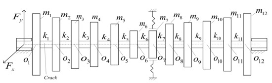
Figure 1.
Rotor model with coupling faults (crack and rub-impact).
Here we assume that the axial and torsional vibrations of the system and the gyroscopic moment are neglectful. are the geometric centers of the discs. are the equivalent lumped masses. are the equivalent damping coefficients at the position of the lumped masses. are the equivalent stiffness of the corresponding discs. Assume that the crack occurs on the shaft between the first and second disc. The rotor model is supported by a pair of liquid-film bearings on both ends.
The schematic diagram of the cracked section is shown in Figure 2a. is the depth of crack, is the intersection angle between the unbalance and the crack normal vector. Law of open and close describes the effects of crack intersection angle to the shaft stiffness. There are three classic models that characterizing the time-varying property of a crack when the rotor is operating: the cosine model [53], square wave model and hybrid one [54].
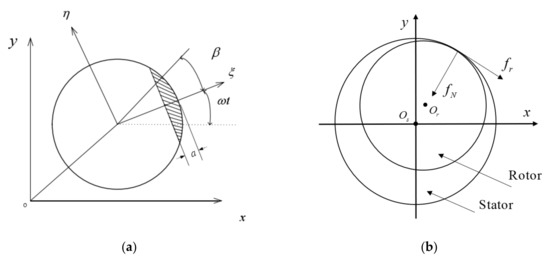
Figure 2.
Schematic diagram of the cracked section and rubbing model. (a) The cracked model. (b) The rub-impact model.
In Figure 2a, the initial intersection angle of the cracked normal vector and x-axis is 0. We consider the case of gravity dominance, the open and close function of crack can be expressed as the function of rotating angle . is the cracked stiffness of rotating shaft, and are the stiffness variations of cracked normal and tangential vectors. The stiffness of rotating shaft with crack is expressed as:
The expression of is shown in Formula (6), this model can select the square wave and cosine model based on the depth of the crack respectively.
The rub-impact model is shown in Figure 2b, it is combined with linear contact force and Coulomb friction [55], the formula is expressed as:
where is radial displacement, is clearance between rotor and stator, is rub-impact stiffness, is frictional coefficient, and represent the rub-impact forces along x and y directions.
The dynamical equation is shown in Formula (8) and the dimensionless process is expressed as follows:
and represent the vibration displacement of x and y directions. The dimensionless equation is expressed as Formula (9). and are the model of dimensionless non-linear oil-film force, , . and are the , directional components of bearing non-linear oil-film force. is the bearing clearance, is the Sommerfeld number. is the lubricating oil viscosity, is the bearing length, is the radius of the bearing, is the external excitation, is the loading, and is the dimensionless time. The detailed values of the corresponding parameters of the rotor system are shown as in the Appendix A. The non-linear oil-film force [56] along and directions can be found in Appendix B. We also provide the formulas of the corresponding parameters in Appendix B.
Equation (9) is the dimensionless form of Equation (8). The dimensionless Equation (9) can be written as Equation (10), in which , the expression of are shown as above:
To facilitate the theory analysis, we implement the Taylor series expansion of the oil-film force, thus can be rewritten as:
For the convenience of calculation, Equation (10) is written as Equation (12) briefly:
In Equation (12), is the damping matrix, is the stiffness matrix, is the force vector, which includes oil-film and external excitation etc. corresponds to in Equation (10).
3. Discussion of the Dynamical Characteristics and Effects of Systematic Parameters
In this section, we will study the non-linear dynamical characteristics of the rotor with the coupling faults by comparing the coupling faults with the single fault (crack or rub-impact). Then we will discuss the effects of the systematic parameters to the coupling fault. Here we define the initial values as , , , , and the integral step is .
3.1. Discussion of the Dynamical Characteristics
Figure 3 shows the four amplitude–frequency curves of the rotor systems with different faults: the original system without faults; the cracked fault; the rub-impact fault and the coupling fault. 1/2 sub-harmonic vibration occurs in the cracked and coupling system at the frequency of , is the natural frequency. The amplitude of the coupling system is apparently higher than the system with only crack fault, which indicates that the rub-impact will increase the response amplitude of the crack. The amplitude of the system with rub-impact bumps up at the frequency of 1000 (nearby ), this result illustrates rub-impact will aggravate the complex motion of the system.
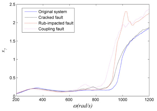
Figure 3.
Comparison of amplitude–frequency curves.
Figure 4 shows the bifurcation diagrams of the rotor systems with different faults: (a) the oil-film fault; (b) the crack fault; (c) the rub-impact fault; (d) the coupling fault. It is clear that the bifurcation behaviors vary with different rotor faults. The obvious period-doubling bifurcation occurs at the second order natural frequency of the cracked fault system. The period-doubling bifurcation also occurs in the coupling fault system, but the amplitude is much larger. When the rotating speed is 1000 rad/s (nearby ), the amplitude of the rub-impact fault system suddenly increases, which indicates that the rub-impact fault can give rise to the complex motion of the system.
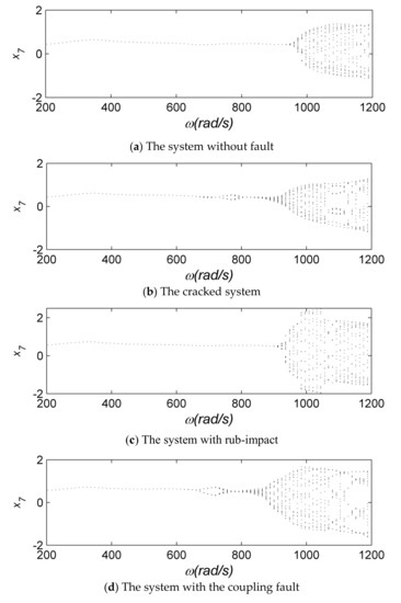
Figure 4.
Bifurcation diagrams.
When (nearby the primary resonance), the time history curves of the four systems are drawn clearly in Figure 5. The curves contain both the transient and steady-state processes. The transient process of the oil-filmed system (Figure 5a) vanishes in about two periods, the other three systems (Figure 5b–d) need three periods. This indicates that the stability of the system with faults can’t be kept in comparison to the normal system. Meanwhile, in Figure 5d, the steady-state signal of the coupling fault is not standard sinusoidal, which has a visible difference in the other three systems.
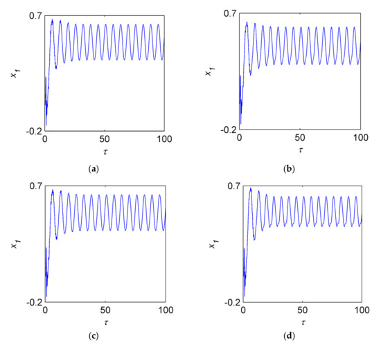
Figure 5.
Time history curves of when . (a) The oil-filmed system. (b) The cracked system. (c) The rub-impacted system. (d) The coupled system.
In Figure 6, it shows the trajectories of the orbit of shaft center of the four systems. The motion curves in (a) and (c) are all elliptical. The major axis and minor axis of ellipse of the oil-filmed system is longer than the rub-impact system. The trajectories of the orbit of shaft center of cracked (b) and coupling (d) faults are the closed curves similar to ellipse, but the bottom is a little narrow. The crack fault is the main reason to change the ellipse of trajectories of the orbit of shaft center as closed curves similar to the ellipse near the primary resonance.

Figure 6.
Trajectories of the orbit of shaft center of when . (a) The oil-filmed system. (b) The cracked system. (c) The rub-impacted system. (d) The coupled system.
We use the comparison of the phase portraits (Figure 7) to verify the results in Figure 6 based on the same initial values and rotating speed. In Figure 7a,c, it is easy to discover that the phase portraits are both the closed curves similar to circle, and the diameter of the oil-filmed system is larger. In the other two figures (Figure 7a,c), the curves are both irregularly closed.
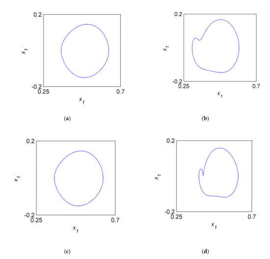
Figure 7.
The phase portraits of when . (a) The oil-filmed system. (b) The cracked system. (c) The rub-impacted system. (d) The coupled system.
Remark 1.
The crack and coupling faults have greater effect to the motion state near the primary resonance. Moreover, the rub-impact fault has more obvious effect to the vibration amplitude at the frequency of primary resonance. The variations of the dynamical characteristics in Figure 5, Figure 6 and Figure 7 can provide theory guidance to the fault diagnosis of the non-linear rotor-bearing system.
Similar to the discussions before, we study the time histories, trajectories of the orbit of shaft center, phase portraits of the four different systems at the frequency of 1/2 sub-harmonic vibration (730 ) in Figure 8, Figure 9 and Figure 10. In Figure 8, the time histories contain the transient process and the stable motion state, the four systems vary from transient to stable state after , so the three different faults have little effect to the dynamical characteristics of the systems near the frequency . The signal is similar to sinusoidal after the oil-filmed (Figure 8a) and cracked system (Figure 8c) leads to periodic motion. The signals of the other two systems (Figure 8b,d) are more complex relative to oil-filmed and cracked systems.
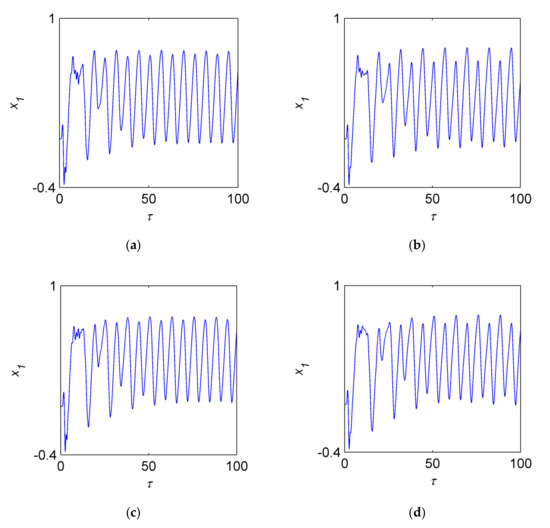
Figure 8.
Time history curves of when . (a) The oil-filmed system. (b) The cracked system. (c) The rub-impacted system. (d) The coupled system.
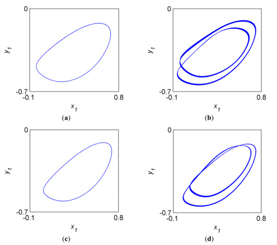
Figure 9.
Trajectories of the orbit of shaft center of when . (a) The oil-filmed system. (b) The cracked system. (c) The rub-impacted system. (d) The coupled system.
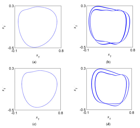
Figure 10.
The phase portraits of when . (a) The oil-filmed system. (b) The cracked system. (c) The rub-impacted system. (d) The coupled system.
Figure 9 analyzes the trajectories of the orbit of shaft center of the four different system when . The motion curves of the oil-filmed and rub-impact systems (Figure 9a,c) are similar to ellipse. In comparison to Figure 9a,c, double-loop curves are embodied in the cracked and coupling systems. There is one intersection in the cracked system and two intersections in the coupling system, this result indicates that the crack fault is a key factor in the appearance of double-loop curves at . The rub-impact fault may affect the topological structures of the double-loop curves.
As is clearly seen in Figure 10a,c, the phase portraits of the oil-filmed and rub-impact systems are the curves similar to ellipse. The curves in Figure 10b,d are both double-loop, the two loops are closer in the cracked system relative to the coupling system. This result also verifies that the crack fault can lead to double-loop curves, the rub-impact fault affects the topological structures of phase portraits.
Remark 2.
In Figure 8, Figure 9 and Figure 10, the crack fault affects more to the rotor system at the frequency of . The signal of cracked fault system is more complex, the double-loop curves occur in both trajectories of the orbit of shaft center and phase portraits, the period-doubling bifurcation occurs in Figure 4b. The rub-impact fault will not affect the natural structures of the cracked characteristics. Hence, the dynamical characteristics near the frequency of can be regarded as the important judgments to verify the crack fault of the rotor-bearing system.
In Figure 11, the four figures (Figure 11a–d) show the time histories of the rotor-bearing models at the frequency of . There exists a certain difference between the four faults of the rotor system. The difference of the time history can provide theory guidance to the fault detection of the rotor system.
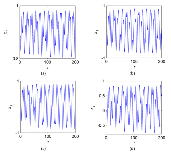
Figure 11.
Time history curves of when . (a) The oil-filmed system. (b) The cracked system. (c) The rub-impacted system. (d) The coupled system.
As is shown in Figure 12, it shows the orbit of shaft center diagrams of the oil-film, crack, rub-impact, coupling fault when (the third order natural frequency). Based on the constraint of the displacement of rub-impact fault, the orbit of shaft center is easier than the other three curves. However, the displacement is the largest, which indicates that the rub-impact fault arouses the larger motion near the third order frequency. The orbit of shaft center of the crack fault is more complex than that of the oil-film fault. The complexity of the orbit of shaft center of the coupling fault is situated between the oil-film fault and crack fault.
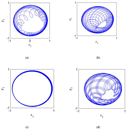
Figure 12.
Trajectories of the orbit of shaft center of when . (a) The oil-filmed system. (b) The cracked system. (c) The rub-impacted system. (d) The coupled system.
Figure 13 shows phase diagrams of oil-film, crack, rub-impact and the coupling systems at the frequency of . Oil-film rotor causes complex motion at this time. The phase diagram of the rub-impact fault is annular narrow band, it is a quasi-periodic attractor. The sort of the four fault cases can be given based on the complexity of the attractor: crack, coupling, oil-film and rub-impact.
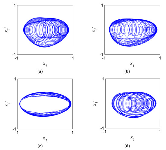
Figure 13.
The phase portraits of when . (a) The oil-filmed system. (b) The cracked system. (c) The rub-impacted system. (d) The coupled system.
Remark 3.
By comparing the results in Figure 11, Figure 12 and Figure 13, we can obtain the conclusions as follows: the crack fault can arouse the 1/2 sub-harmonic vibration, the violent vibration at the frequency of can be aroused by the rub-impact fault. At the frequency of primary resonance, the rub-impact and coupling fault may give rise to the reducing of the first order critical speed, while the crack and coupling fault may cause the structural variation of trajectories of the orbit of shaft center and phase portraits. The crack can restrain the vibration amplitude at the frequency of in the coupling system, the crack also arouses the trajectories of the orbit of shaft center and attractor more complex.
Remark 4.
The shaft stiffness varies with the open and close of crack periodically when the crack fault occurs, which may make the trajectories of the orbit of shaft center and attractor structure more complex. When the full annular rub occurs, the vibration amplitude is restrained. Meanwhile, the frictional force and restriction will reduce the complexity of the attractor.
3.2. The Effects of Systematic Parameters
We will discuss the effects of systematic parameters of the rotor system to the dynamical characteristics of the coupling fault. The systematic parameters include cracked depth, clearance between rotor and stator, stator stiffness, eccentricity. The bifurcation and amplitude–frequency behaviors will be provided as the values of the systematic parameters vary.
3.2.1. The Cracked Depth
The effect of the cracked depth variation on dynamical characteristics of the coupling fault is investigated in this section. As is shown in Figure 14a,b, they reflect the bifurcation diagrams of the coupling fault systems with the cracked depth and . Figure 15 shows the comparison of frequency-amplitude curves of two cracked depths. As the cracked depth decreases, the stiffness variation decreases correspondingly, so the first order critical speed of the coupling fault rotor slightly increases. The period-doubling bifurcation vanishes at the frequency of , the 1/2 sub-harmonic vibration amplitude of the relevant amplitude–frequency characteristic decreases at the same time (Figure 15). Since the crack fault characteristic does not play the main role and even vanishes, the rub-impact fault emerges, the vibration amplitude suddenly increases at the frequency of . This change demonstrates the crack is the main factor to generate 1/2 sub-harmonic vibration in the coupling system again, there will be more effect with the increase of the cracked depth. The rub-impact fault will result in the amplitude of the coupling fault peaking at the frequency of , there is reversible inhibition of the crack to the amplitude aroused by the rub-impact. The restrain will be stronger as the cracked depth increases. When , the cracked depth will have little impact to the amplitude based on the comparison of the amplitude–frequency curves (Figure 15). In comparison to the bifurcation diagrams (Figure 14), the complex motion state of the system changes.
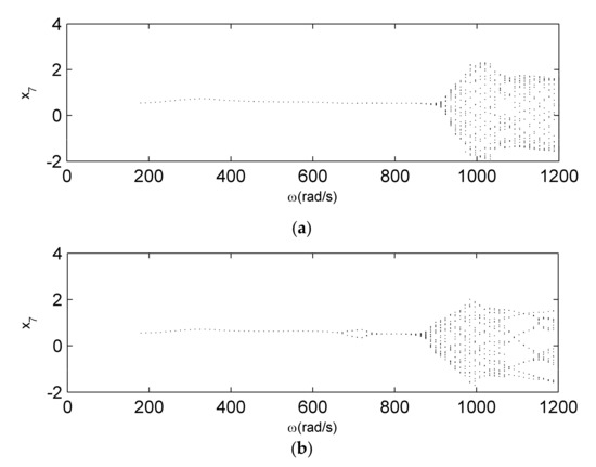
Figure 14.
Bifurcation diagrams for coupled fault system. (a) . (b) .
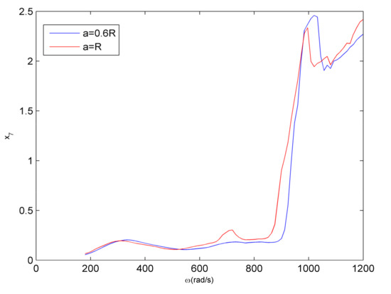
Figure 15.
Comparison of the amplitude–frequency curves.
3.2.2. Clearance between Rotor and Stator
This section discusses the effects of clearance between rotor and stator to the coupling fault. Similarly, Figure 16 and Figure 17 present the bifurcation and amplitude–frequency when the clearance is 0.12 and 0.18, respectively. When the clearance varies, the clearance has little impact on the vibration amplitude and critical speed of the coupling system. Near the frequency of , the amplitude of 1/2 sub-harmonic resonance decreases as the clearance decreases, the amplitudes of the systems with different clearance are similar when . The amplitude will have a sharp increase as the clearance decreases at the frequency of , the rub-impact fault characteristic enhanced obviously, which once verifies that the sudden increase of the amplitude of the coupling fault system is primarily caused by the rub-impact fault. At the high frequency (over ), the amplitude increases a little when the clearance decreases. The topological structures of the bifurcation diagram will be more complex in comparison to Figure 16b.
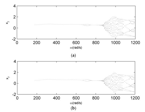
Figure 16.
Bifurcation diagrams for coupled fault system. (a) . (b) .
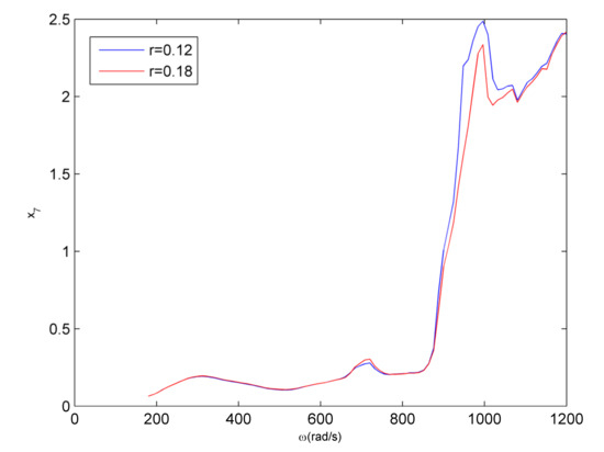
Figure 17.
Comparison of the amplitude–frequency curves.
3.2.3. Stator Stiffness
The effects of the stator stiffness variation to the bifurcation behaviors and amplitude–frequency are studied in this section. We select two different parameter values to discuss the comparison of bifurcation (Figure 18) and amplitude–frequency (Figure 19) of the coupling fault system: the first is , the second is . In Figure 19, we can see clearly that the variation of the stator stiffness has little impact on the primary frequency, vibration amplitude and critical speed. 1/2 sub-harmonic resonance amplitude increases as the stiffness decreases. At the frequency of , the amplitude changes obviously when the stiffness decreases. The complex motion region is simpler when the stiffness is .
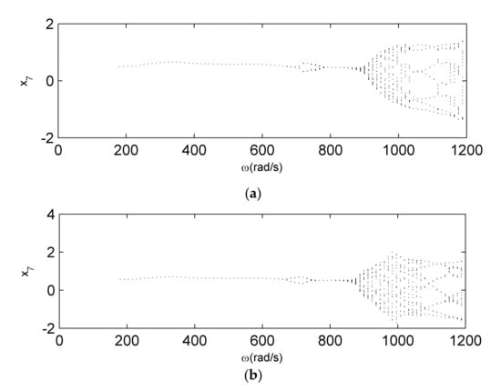
Figure 18.
Bifurcation diagrams for coupled fault system. (a) . (b) .
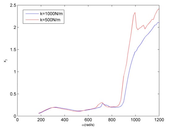
Figure 19.
Comparison of the amplitude–frequency curves.
3.2.4. Eccentricity
Finally, we study the effects of the eccentricity variation to the coupling fault system. Figure 20 and Figure 21 present the comparison of bifurcation and amplitude–frequency of two different eccentricities (0.00015 mm and 0.00012 mm). As is shown in Figure 21, the amplitude increases when the eccentricity magnifies at the frequency of primary resonance. 1/2 sub-harmonic resonance is more obvious near the frequency of , it is clear that the annulus of the period-doubling bifurcation is larger. When the frequency is over , the amplitude decreases as the eccentricity increases, this result indicates that increasing the eccentricity appropriately can improve the stability of the system under a certain speed. However, in the high frequency region, the bifurcation behaviors will be more complex when the eccentricity increases, in other words, the non-linear dynamic characteristics will be more complex. As is discussed above, the eccentricity of the system has more impact to dynamical characteristic of the amplitude–frequency and bifurcation at the frequencies of primary resonance, , high frequency. The eccentricity may affect the visualizations of different faults at each frequency range.
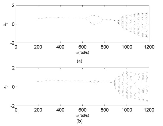
Figure 20.
Bifurcation diagrams for coupled fault system. (a) . (b) .
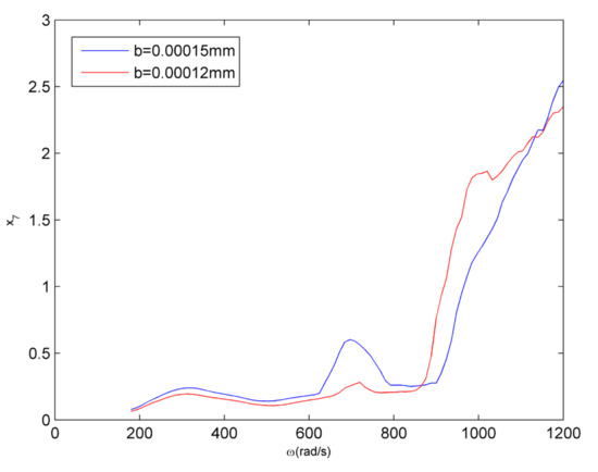
Figure 21.
Comparison of the amplitude–frequency curves.
Remark 5.
The systematic parameters play a key role in the rotor models, the variations of the parameters will affect the dynamical characteristics of the rotor-bearing system. We make a preliminary study on the effects of cracked depth, clearance between rotor and stator, stator stiffness, eccentricity to the bifurcation diagrams and amplitude–frequency curves. This research is only a beginning to discuss the variations of the dynamical characteristics with the systematic parameters. We can also use the frequency-spectrum analysis to describe the effects of the variations of the parameters.
4. The Optimal Reduced Model Based on the POM Energy
The first few order POMs pertaining to the rotating speed of the rotor will be discussed to confirm the dimension of the reduced model in this section.
In Figure 22, it shows the first three order POM energy curve of the 24-DOFs rotor model with the coupling fault. It is clear that the three order POMs occupy 98.7% energy when the rotating speed is about 1120 , so we can obtain the optimal order reduction model at this speed based on the POM energy method. The POM energy method has been applied in Ref. [50], then we use the TPOD method in Section 2.1 to reduce the 24-DOFs rotor model to a 3-DOFs one.
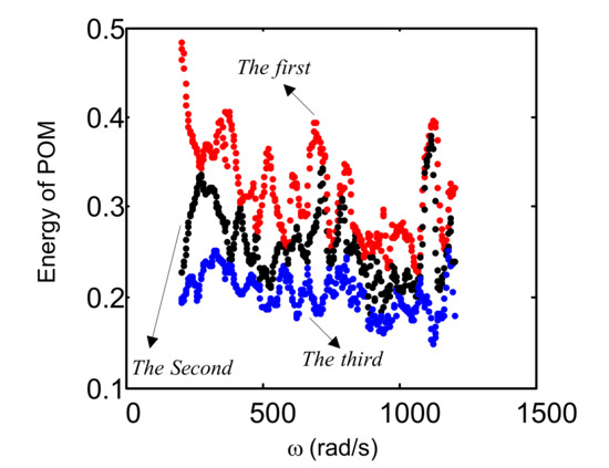
Figure 22.
The POM (proper orthogonal mode) energy of the 24-DOFs (degrees of freedom) model with coupling fault.
The dynamical equation of the order reduction model can be expressed as:
Remark 6.
The POM can provide the physical significance of the TPOD method. The POM energy can reveal the amount of occupation of the dynamical characteristics of the reduced model relative to the original one. The POM energy method is applied to confirm the dimension of the order reduction model. Then we use the TPOD method to get the optimal reduced model at the corresponding rotating speed.
5. The Efficiency of the Order Reduction Method
In this section, we will discuss the efficiency of the order reduction method via the bifurcation analysis of the original and the reduced system.
On the basis of the POM energy curve (Figure 22), we can obtain the 3-DOFs reduced model when the rotating speed is 1120 . As is shown in Figure 23, we can see clearly that the reduced system (Figure 23b) preserves the period-doubling bifurcation, the rotating speed of complex motion and the topological structure of the original one (Figure 23a). The comparison of the bifurcation diagrams verifies the efficiency of the TPOD method, we can also use other dynamical behaviors (phase portraits, amplitude–frequency curve, etc.) to discuss the efficiency [49,50], we don’t state one by one here.
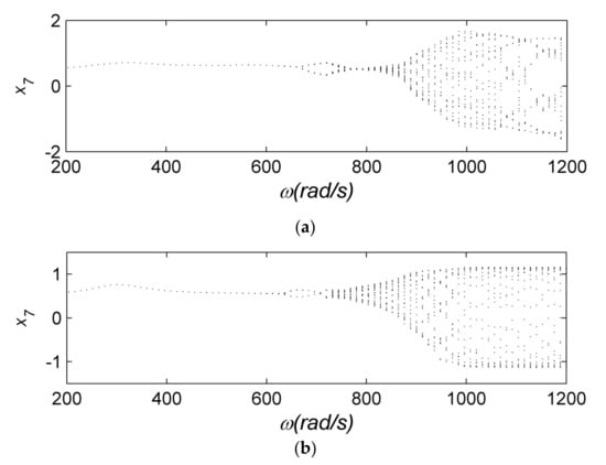
Figure 23.
Bifurcation diagrams. (a) The original system. (b) The reduced system.
Remar 7.
The reduced order reduction model obtained by the TPOD method preserves the dynamical characteristics of the original one well. The TPOD method is proposed by the present authors, it is applied in the rotor models supported by the sliding bearings or ball bearings with looseness. The efficiency of the order reduction method applied in the rotor system with coupling fault further generalizes this method. The Runge-Kutta method is used to calculate the dynamic response, and we can obtain the results in Figure 3, Figure 4, Figure 5, Figure 6, Figure 7, Figure 8, Figure 9, Figure 10, Figure 11, Figure 12, Figure 13, Figure 14, Figure 15, Figure 16, Figure 17, Figure 18, Figure 19, Figure 20, Figure 21, Figure 22 and Figure 23. It is promising to adapt this method to the uncertainty quantification of faulted rotor systems with parametric variabilities [57,58,59,60]. Fortran Language is used to solve the dynamic equation.
6. Conclusions and Outlooks
The non-linear dynamic characteristics of the rotor system with the coupling faults have been discussed in this paper. A 24-DOFs rotor system supported by a pair of sliding bearings with both crack and rub-impact faults has been established by the Newton’s second law. The coupling faults have been studied via comparing the single fault (crack or rub-impact). The effects of the systematic parameters (cracked depth, clearance between rotor and stator, stator stiffness, eccentricity) to the coupling faults have also been presented by comparing with the bifurcation and amplitude–frequency characteristics. The POM energy method has been used to confirm the DOF number of the reduced system. The TPOD has been applied to reduce the original system to a 3-DOFs one, the efficiency of the optimal order reduction model has been verified via the comparison of the bifurcation diagrams. The POM energy is a direct method to obtain the optimal reduced system of high-dimensional non-linear dynamic system. The dynamic characteristics analysis of the rotor system with coupling faults and the applications of the TPOD method can provide qualitative guidance to the common faults in rotor system and prior information of fault diagnosis.
Further studies on this subject are being carried out by the present authors in the three aspects: the first is to study the dynamical characteristics of the ball bearing rotor model with the coupling faults; the second is to study the coupling faults of the rotor system with uncertainties based on the polynomial dimensional decomposition and other methods.
Author Contributions
Data curation, N.W., K.Z. and C.F.; Formal analysis, K.L., C.F. and Y.J.; Funding acquisition, K.L.; Investigation, N.W.; Methodology, K.L., N.W., C.F. and Y.J.; Project administration, K.L. and Y.Y.; Resources, Y.J. and H.Z.; Software, K.Z., Y.Y. and H.Z.; Visualization, H.Z.; Writing—Original draft, K.L. and Y.J.; Writing—Review & editing, K.Z. and Y.Y. All authors have read and agreed to the published version of the manuscript.
Funding
This research was funded by National Natural Science Foundation of China (Grant No. 12072263, 11802235, 11972295), the Natural Science Foundation of Shaanxi Province (Grant No. 2020JQ-129) and Aviation Engine Innovation Center of National Defense Science, Technology and Industry (Grant No. CXZX-2019-001).
Conflicts of Interest
The authors declare that they have no conflict of interest.
Nomenclature
| equivalent damping matrix | |
| equivalent stiffness matrix | |
| equivalent force vector | |
| number of DOFs | |
| geometric centers of the discs | |
| equivalent lumped masses | |
| equivalent damping coefficients | |
| equivalent stiffness | |
| rotating speed | |
| depth of crack | |
| intersection angle between unbalance and crack normal vector | |
| stiffness of cracked rotating shaft | |
| , | stiffness variations of cracked normal and tangential vectors |
| radial displacement | |
| clearance between rotor and stator | |
| rub-impact stiffness | |
| frictional coefficient | |
| , | rub-impact forces along x and y directions |
| , | vibration displacement of x and y directions |
| , | dimensionless non-linear oil-film force |
| bearing clearance | |
| s | Sommerfeld number |
| lubricating oil viscosity | |
| bearing length | |
| radius of the bearing | |
| loading | |
| dimensionless time |
Appendix A
Appendix B
References
- Sinou, J.J.; Lees, A.W. The influence of cracks in rotating shafts. J. Sound Vib. 2005, 285, 1015–1037. [Google Scholar] [CrossRef]
- Ren, Z.; Zhou, S.; Chunhui, E.; Gong, M.; Li, B.; Wen, B. Crack fault diagnosis of rotor systems using wavelet transform. Comput. Electr. Eng. 2015, 45, 33–41. [Google Scholar] [CrossRef]
- Sinou, J.J. Detection of cracks in rotor based on the 2× and 3× super-harmonic frequency components and the crack-unbalance interactions. Commun. Nonlinear Sci. Numer. Simulat. 2008, 13, 2024–2040. [Google Scholar] [CrossRef]
- Hou, L.; Chen, Y.S.; Lu, Z.Y.; Li, Z.G. Bifurcation analysis for 2:1 and 3:1 super-harmonic resonances of an aircraft cracked rotor system due to maneuver load. Nonlinear Dyn. 2015, 81, 531–547. [Google Scholar] [CrossRef]
- Fu, C.; Xu, Y.; Yang, Y.; Lu, K.; Gu, F.; Ball, A. Dynamics analysis of a hollow-shaft rotor system with an open crack under model uncertainties. Commun. Nonlinear Sci. Numer. Simulat. 2020, 83, 105102. [Google Scholar] [CrossRef]
- Ma, H.; Yu, T. Time-frequency features of two types of coupled rub-impact faults in rotor systems. J. Sound Vib. 2009, 321, 1109–1128. [Google Scholar] [CrossRef]
- Jacquet, R.G.; Torkhani, M.; Cartraud, P.; Thouverez, F.; Baranger, T.N.; Herran, M.; Gibert, C.; Baguet, S.; Almeida, P.; Peletan, L. Rotor to stator contacts in turbomachines. Review and application. Mech. Syst. Signal Process 2013, 40, 401–420. [Google Scholar] [CrossRef]
- Khanlo, H.M.; Ghayour, M.; Ziaei, R.S. Chaotic vibration analysis of rotating, flexible, continuous shaft-disk system with a rub-impact between the disk and the stator. Commun. Nonlinear Sci. Numer. Simulat. 2011, 16, 566–582. [Google Scholar] [CrossRef]
- Hou, L.; Chen, Y.S.; Cao, Q.J. Nonlinear vibration phenomenon of an aircraft rub-impact rotor system due to hovering flight. Commun. Nonlinear Sci. Numer. Simulat. 2014, 19, 286–297. [Google Scholar] [CrossRef]
- An, X.L.; Zhang, F. Pedestal looseness fault diagnosis in a rotating machine based on variational mode decomposition. Proc. Inst. Mech. Eng. Part C J. Mech. Eng. Sci. 2017, 231, 2493–2502. [Google Scholar] [CrossRef]
- Chu, F.L.; Tang, Y. Stability and nonlinear responses of a rotor-bearing system with pedestal looseness. J. Sound Vib. 2001, 241, 879–893. [Google Scholar] [CrossRef]
- Ma, H.; Zhao, X.Y.; Teng, Y.N.; Wen, B.C. Analysis of dynamic characteristics for a rotor system with pedestal looseness. Shock Vib. 2011, 18, 13–27. [Google Scholar] [CrossRef]
- Ji, Z.; Zu, J.W. Method of multiple scales for vibration analysis of rotor-shaft systems with nonlinear bearing pedestal model. J. Sound Vib. 1998, 218, 293–305. [Google Scholar] [CrossRef]
- Dolenc, B.; Boskoski, P.; Juričić, Đ. Distributed bearing fault diagnosis based on vibration analysis. Mech. Syst. Signal Process 2016, 66, 521–532. [Google Scholar] [CrossRef]
- Sekhar, A.S. Crack detection and monitoring in a rotor supported on fluid film bearings: Start-up vs run-down. Mech. Syst. Signal Process 2003, 17, 897–901. [Google Scholar] [CrossRef]
- Zhao, S.B.; Ren, X.M.; Deng, W.Q.; Lu, K.; Yang, Y.F.; Fu, C. A transient characteristic-based balancing method of rotor system without trail weights. Mech. Syst. Signal Process 2020, 148, 107117. [Google Scholar] [CrossRef]
- Sarangi, S.; Kdekar, M. Misalignment faults detection in an induction motor based on multi-scale entropy and artificial neural network. Electr. Pow. Compo. Sys. 2016, 44, 916–927. [Google Scholar]
- Didier, J.; Sinou, J.J.; Faverjon, B. Study of the non-linear dynamic response of a rotor system with faults and uncertainties. J. Sound Vib. 2012, 331, 671–703. [Google Scholar] [CrossRef]
- Lu, K.; Jin, Y.L.; Huang, P.F.; Zhang, F.; Zhang, H.P.; Fu, C.; Chen, Y.S. The applications of POD method in dual rotor-bearing systems with coupling misalignment. Mech. Syst. Signal Process 2020, 150, 107236. [Google Scholar] [CrossRef]
- Fu, C.; Ren, X.M.; Yang, Y.F. Vibration analysis of rotors under uncertainty based on Legendre series. J. Vib. Eng. Technol. 2019, 7, 43–51. [Google Scholar] [CrossRef]
- Ma, Y.; Liu, H.; Zhu, Y.; Wang, F.; Luo, Z. The NARX model-based system identification on nonlinear, rotor-bearing systems. Appl. Sci. 2017, 7, 911. [Google Scholar] [CrossRef]
- Wan, Z.; Wang, Y.; Chen, B.; Dou, Y.; Wei, X. The Vibration of a Transversely Cracked Rotor Supported by Anisotropic Journal Bearings with Speed-Dependent Characteristic. Appl. Sci. 2020, 10, 5617. [Google Scholar] [CrossRef]
- Deng, H.; Diao, Y.; Zhang, J.; Zhang, P.; Ma, M.; Zhong, X.; Yu, L. Three-dimensional identification for unbalanced mass of rotor systems in operation. Appl. Sci. 2018, 8, 173. [Google Scholar] [CrossRef]
- Alho, A.; Uggla, C. Global dynamics and inflationary center manifold and slow-roll approximants. J. Math. Phys. 2015, 56, 012502. [Google Scholar] [CrossRef]
- Valls, C. Center problem in the center manifold for quadratic and cubic differential systems in R3. Appl. Math. Comput. 2015, 251, 180–191. [Google Scholar]
- Verdugo, A.; Rand, R. Center manifold analysis of a DDE model of gene expression. Commun. Nonlinear Sci. Numer. Simul. 2008, 13, 1112–1120. [Google Scholar] [CrossRef]
- Kazufumi, I.; Karl, K. Reduced-order optimal control based on approximate inertial manifolds for nonlinear dynamical systems. SIAM J. Numer. Anal. 2008, 46, 2867–2891. [Google Scholar]
- Foial, C.; Sell, G.; Teman, R. Inertial manifolds for nonlinear evolutionary equations. J. Differ. Equ. 1988, 73, 93–114. [Google Scholar]
- Marion, M. Approximate inertial manifolds for reaction–diffusion equations in high space dimension. Dyn. Differ. Equ. 1989, 1, 245–267. [Google Scholar] [CrossRef]
- Kunisch, K.; Volkwein, S. Galerkin proper orthogonal decomposition methods for parabolic problems. Numer. Math. 2001, 90, 117–148. [Google Scholar] [CrossRef]
- Marion, M.; Temam, R. Nonlinear Galerkin methods. SIAM J. Numer. Anal. 1989, 26, 1139–1157. [Google Scholar] [CrossRef]
- Carlberg, K.; Bou-Mosleh, C.; Farhat, C. Efficient non-linear model reduction via a least-squares Petrove-Galerkin projection and compressive tensor approximations. Int. J. Numer. Methods Eng. 2011, 86, 155–181. [Google Scholar] [CrossRef]
- Guo, S.J.; Yan, S.L. Hopf bifurcation in a diffusive Lotka- Volterra type system with nonlocal delay effect. J. Differ. Equ. 2016, 260, 781–817. [Google Scholar] [CrossRef]
- Nikolic, M.; Rajkovic, M. Bifurcations in nonlinear models of fluid-conveying pipes supported at both ends. J. Fluids Struct. 2006, 22, 173–195. [Google Scholar] [CrossRef]
- Stefanescu, R.; Sandu, A.; Navon, I.M. POD/DEIM reduced-order strategies for efficient four dimensional variational data assimilation. J. Comput. Phys. 2015, 295, 569–595. [Google Scholar] [CrossRef]
- Kappagantu, R.; Feeny, B.F. Part 1: Dynamical characterization of a frictionally exited beam. Nonlinear Dyn. 2000, 22, 317–333. [Google Scholar] [CrossRef]
- Amabili, M.; Touze, C. Reduced-order models for nonlinear vibrations of fluid-filled circular cylindrical shells: Comparison of POD and asymptotic nonlinear normal modes methods. J. Fluids Struct. 2007, 23, 885–903. [Google Scholar] [CrossRef]
- Liang, Y.C.; Lee, H.P.; Lim, S.P.; Lin, W.Z.; Lee, K.H.; Wu, C.G. Proper orthogonal decomposition and its applications, part I: Theory. J. Sound Vib. 2002, 252, 527–544. [Google Scholar] [CrossRef]
- Stefanescu, R.; Navon, I.M. POD/DEIM nonlinear model order reduction of an ADI implicit shallow water equations model. J. Comput. Phys. 2013, 237, 95–114. [Google Scholar] [CrossRef]
- Stefanescu, R.; Sandu, A.; Navon, I.M. Comparison of POD reduced order strategies for the nonlinear 2D shallow water equations. Int. J. Numer. Methods Fluids 2014, 76, 497–521. [Google Scholar] [CrossRef]
- Yang, H.L.; Radons, G. Geometry of inertial manifolds probed via a Lyapunov projection method. Phys. Rev. Lett. 2012, 108, 154101. [Google Scholar] [CrossRef] [PubMed]
- Hamilton, N.; Tutkun, M.; Cal, R.B. Low-order representations of the canonical wind turbine array boundary layer via double proper orthogonal decomposition. Phys. Fluids 2016, 28, 025103. [Google Scholar] [CrossRef]
- Siegel, S.; Seidel, J.; Fagley, C.; Luchtenburg, D.M.; Cohen, K.; Mclaughlin, T. Low-dimensional modeling of a transient cylinder wake using double proper orthogonal decomposition. J. Fluid Mech. 2008, 610, 1–42. [Google Scholar] [CrossRef]
- Rega, G.; Troger, H. Dimension reduction of dynamical systems: Methods, models, applications. Nonlinear Dyn. 2005, 41, 1–15. [Google Scholar] [CrossRef]
- Lu, K.; Jin, Y.L.; Chen, Y.S.; Yang, Y.F.; Hou, L.; Zhang, Z.Y.; Li, Z.G.; Fu, C. Review for order reduction based on proper orthogonal decomposition and outlooks of applications in mechanical systems. Mech. Syst. Signal Process 2019, 123, 264–297. [Google Scholar] [CrossRef]
- Holmes, P.J.; Lumley, L.; Berkooz, G. Turbulence, Coherent Structures, Dynamical Systems and Symmetry; Cambridge University Press: Cambridge, UK, 2012. [Google Scholar]
- Lu, K.; Yu, H.; Chen, Y.S.; Cao, Q.J.; Hou, L. A modified nonlinear POD method for order reduction based on transient time series. Nonlinear Dyn. 2015, 79, 1195–1206. [Google Scholar] [CrossRef]
- Yu, H.; Chen, Y.S.; Cao, Q.J. Bifurcation analysis for nonlinear multi-degree-of-freedom rotor system with liquid-film lubricated bearings. App. Math. Mech. Engl. Ed. 2013, 34, 777–790. [Google Scholar] [CrossRef]
- Lu, K.; Jin, Y.L.; Chen, Y.S.; Cao, Q.J.; Zhang, Z.Y. Stability analysis of reduced rotor pedestal looseness fault model. Nonlinear Dyn. 2015, 82, 1611–1622. [Google Scholar] [CrossRef]
- Lu, K.; Chen, Y.S.; Jin, Y.L.; Hou, L. Application of the transient proper orthogonal decomposition method for order reduction of rotor systems with faults. Nonlinear Dyn. 2016, 86, 1913–1926. [Google Scholar] [CrossRef]
- Lu, K.; Chen, Y.S.; Cao, Q.J.; Hou, L. Bifurcation analysis of reduced rotor model based on nonlinear transient POD method. Int. J. Nonlinear Mech. 2017, 89, 83–92. [Google Scholar] [CrossRef]
- Lu, K.; Lu, Z.Y.; Chen, Y.S. Comparative study of two order reduction methods for high-dimensional rotor systems. Int. J. Nonlinear Mech. 2018, 106, 330–334. [Google Scholar] [CrossRef]
- Sinou, J.J.; Faverjon, B. The vibration signature of chordal cracks in a rotor system including uncertainties. J. Sound Vib. 2012, 331, 138–154. [Google Scholar] [CrossRef]
- Lin, Y.L.; Chu, F.L. Stiffness Models for the Cracked Shaft of the Rotor System. J. Mech. Eng. 2008, 44, 114–120. [Google Scholar] [CrossRef]
- Jiang, J.; Ulbrich, H. Stability analysis of sliding whirling nonlinear Jeffcott rotor with cross-coupling stiffness coefficients. Nonlinear Dyn. 2001, 24, 269–283. [Google Scholar] [CrossRef]
- Adiletta, G.; Guido, A.R.; Rossi, C. Chaotic motions of a rigid rotor in short journal bearings. Nonlinear Dyn. 1996, 10, 251–269. [Google Scholar] [CrossRef]
- Fu, C.; Xu, Y.; Yang, Y.; Lu, K.; Gu, F.; Ball, A. Response analysis of an accelerating unbalanced rotating system with both random and interval variables. J. Sound Vib. 2020, 466, 115047. [Google Scholar] [CrossRef]
- Lu, K. Statistical moment analysis of multi-degree of freedom dynamic system based on polynomial dimensional decomposition method. Nonlinear Dyn. 2018, 93, 2003–2018. [Google Scholar] [CrossRef]
- Lu, K.; Yang, Y.F.; Xia, Y.B.; Fu, C. Statistical moment analysis of nonlinear rotor system with multi uncertain variables. Mech. Syst. Signal Process 2019, 116, 1029–1041. [Google Scholar] [CrossRef]
- Fu, C.; Feng, G.J.; Ma, J.J.; Lu, K.; Yang, Y.F.; Gu, F.S. Predicting the dynamic response of dual-rotor system subject to interval parametric uncertainties based on the non-intrusive mathematical metamodel. Mathematics 2020, 8, 756. [Google Scholar] [CrossRef]


Publisher’s Note: MDPI stays neutral with regard to jurisdictional claims in published maps and institutional affiliations. |
© 2020 by the authors. Licensee MDPI, Basel, Switzerland. This article is an open access article distributed under the terms and conditions of the Creative Commons Attribution (CC BY) license (http://creativecommons.org/licenses/by/4.0/).