Deep Convolutional Neural Networks Object Detector for Real-Time Waste Identification

Abstract

This paper presents an extensive research carried out for enhancing the performances of convolutional neural network (CNN) object detectors applied to municipal waste identification. In order to obtain an accurate and fast CNN architecture, several types of Single Shot Detectors (SSD) and Regional Proposal Networks (RPN) have been fine-tuned on the TrashNet database. The network with the best performances is executed on one autonomous robot system, which is able to collect detected waste from the ground based on the CNN feedback. For this type of application, a precise identification of municipal waste objects is very important. In order to develop a straightforward pipeline for waste detection, the paper focuses on boosting the performance of pre-trained CNN Object Detectors, in terms of precision, generalization, and detection speed, using different loss optimization methods, database augmentation, and asynchronous threading at inference time. The pipeline consists of data augmentation at the training time followed by CNN feature extraction and box predictor modules for localization and classification at different feature map sizes. The trained model is generated for inference afterwards. The experiments revealed better performances than all other Object Detectors trained on TrashNet or other garbage datasets with a precision of 97.63% accuracy for SSD and 95.76% accuracy for Faster R-CNN, respectively. In order to find the optimal higher and lower bounds of our learning rate where the network is actually learning, we trained our model for several epochs, updating the learning rate after each epoch, starting from 1 × 10⁻¹⁰ and decreasing it until reaching 1 × 10⁻¹.

1. Introduction

Municipal waste sorting is becoming an important matter in cities across the European Union (EU) and beyond. The most recent data showed that in the EU, 786 million tones of waste, excluding major mineral waste, were generated in 2016, equivalent to 35 % of the total waste generated. This means that in relation to population size, the EU generated, on average, 1.8 tones per inhabitant of waste, excluding major mineral waste, in 2016 [1]. Roughly half of the waste (52.6 %) went through different recovery operations: recycling (36.7 % of the total recovered waste), backfilling (10.1 %), or energy recovery (5.8 %). The remaining 47.4 % was landfilled, incinerated without energy recovery, or disposed.

By 2020, the recycling of waste materials such paper, metal, plastic, and glass from households and possibly from other origins was forecasted to a minimum of overall 50% by weight. By 2035, the target is increased to 65% [2]. The latest EU report, from 2016, shows that the average amount of municipal waste that has been recycled was 45%.

One method to maximize recycling is to use autonomous systems which must accurately sort the waste in a short amount of time. One type of autonomous system is the mobile robot used for collecting waste from the ground, which has been developed by our team in collaboration with mechatronic and computer science researchers [3]. The objects that make up the trash are detected using a camera mounted on top of the robotic system and are processed for identification using computer vision and deep neural network models.

The convolutional neural network (CNN) model with the best performance will be embedded on an autonomous mobile robot equipped with an x–y–z robotic manipulator (Festo planar x–y surface gantry plus a vertical electrical slide on z axis), supplied only by DC 24 V for increased autonomy, the end-effector being a Festo electric parallel gripper. The gripper is intended to collect waste objects from the ground and to manipulate them to a box container placed into the mobile robot. In order to identify the municipal waste objects to be collected, an image acquisition and processing system is needed. The image acquisition can be performed using various cameras; in our case, two different designs are tested in parallel: a Festo specialized camera type SBPA-R2-C-U3-2E2A-CS with a CECC-X-M1-MV camera controller and an Omni Vision OV5647 camera with a Raspberry Pi 3+ controller, with a dual-core processor of 1 GHz frequency and 1 GB RAM. In order to reduce the inference time, a USB neural processing device (Neural Compute Stick v2) is added to the second design of the image processing system. There are some other research works that focus on developing robotic systems for autonomous collection and classification of trash [4] or for identification of construction waste such as nails and screws [5]. The implementation of a neural network model on the mobile robot and other aspects of this autonomous sorting framework is not the scope of the paper.

In order to obtain an efficient deep neural network model, the research focuses on boosting the performance of pre-trained Convolutional Neural Network Object Detectors, in terms of precision, generalization, and detection speed, using loss optimization methods, data augmentation, or asynchronous threading at inference time. The model with the best performance will be embedded in a robotic application for waste sorting and collecting from the ground.

The images in the dataset are pre-processed at the training time in order to improve generalization and to extend the dataset. After pre-processing, the images are transferred to the object detectors feature extractor CNN. The proposals of the feature extractors will be the input for the box predictor modules, which will be responsible for localization and classification at different feature map sizes. The performance of the object detector CNN depends on several parameters such as data augmentation, the CNN model, number of images in training/testing dataset, loss optimization, hyper-parameters adjusting, evaluation metrics, transfer learning, fine-tuning, etc. Thus, in order to develop an accurate and real-time architecture, a complex set of actions needs to be carried out. In addition to enhancing the capabilities of object detectors for waste identification and sorting in terms of precision and inference time, the paper presents an in-depth study on the performance of several artificial intelligence methods applied to trash classification.

This paper focuses on object identification based on municipal waste images, more precisely the AI techniques used for localization and classification. The goal is to obtain a real-time and accurate CNN object detector which will be able to correctly classify and locate municipal waste, in order to be identified and picked up by the autonomous mobile robot system. A preliminary study in the area of waste sorting using deep learning has been performed by our team in a previous paper [6]. More precisely, pre-trained CNN architectures have been evaluated on a custom trash test dataset, created in under laboratory conditions, with a high degree of variance (high degree of transparency, uncommon positions, lower resolution, cropped or blocked images), in order to test the real generalization of the models outside the training and testing dataset. This previous research has shown that the most accurate model at inference time in terms of the confidence score obtained on the custom dataset is the Single Shot Detectors (SSD) architecture with MobileNetV2 base network pre-trained on the COCO (Common Objects in COntext) dataset and fine-tuned on the PASCAL Visual Object Classes (VOC) dataset. Based on these first results, this current research continues the study by training the best models on the TrashNet dataset using transfer learning and fine-tuning, data augmentation, regularization, and finding the optimum limits of the learning rate.

In the literature, there are several research works developed in the area of waste sorting using deep learning. The first important results in waste sorting using deep learning were obtained in [7]. The authors developed a database for municipal waste, called TrashNet and used it to train two classifiers: one support vector machine (SVM) and a CNN very similar to the AlexNet model with the Softmax classifier. SVM performed better with an accuracy of 63%, while CNN did not learn well due to hyper-parameter setup. Following the results of this research, a better mean average precision of 68.3% has been obtained [8] using Faster R-CNN and augmentation of the dataset. In [9], a VGG-16 CNN has been used for training and a validation accuracy of 88.42% has been obtained, overfitting the CNN, where some adjustments of the hyper-parameters, architecture, or classification on the fully connected layers have been performed. Newer research on the TrashNet dataset has provided better results. For example, in [10], a Faster R-CNN object detector based on Inception V2 and pre-trained on the COCO dataset has been tested. The results showed a precision of 84.2% and a recall of 87.8%. Using DenseNet121 and Inception-ResNetV2, a test accuracy of 95% and 87%, respectively, has been obtained. In the same paper, the new model, RecycleNet, had shown 81% test accuracy [11]. In [12], the results showed a test accuracy of 93% using a pre-trained VGG-16 network. O. Adedeji and Zenghui Wang used a ResNet50 network with an SVM classifier and obtained 87% accuracy [13]. In [14], the automation of Waste Sorting with Deep Learning has achieved 86%, but the best results, so far, are obtained by [15] using MobileNetV2 for feature extraction and an SVM classifier, with an accuracy of 98.7%. However, this paper has not been peer-reviewed yet. There are some other research works that used different garbage datasets, e.g., in [16], a custom model has been developed and a lightweight neural network based on the AlexNet-SSD model has been used for Garbage Detection, while in [17], a custom dataset has been used for training a multilayer hybrid deep learning model for waste classification and recycling. Most of these methods output only the presence and classification of the object in the picture. In terms of CNN used for object recognition by applying image segmentation, the research in [18] deals with the detecting aluminum profiles within images, using hierarchical representations such as those based on deep learning methods.

Taking into account that municipal waste usually contains a clutter of different waste types, it is necessary to identify as many objects as possible in the image. Moreover, for collecting and sorting waste using a mobile robot, object localization in the image is needed. In order to obtain the localization, object detectors such as Single Shot Detectors, regional proposals (Faster R-CNN), or Mask networks (Mask R-CNN) can be used. In this paper, SSD and Faster R-CNN architectures have been chosen for object detection. Compared to Image Classifiers, which assign a class label to an image, Object Detectors are more challenging as they add the localization of the objects in an image by drawing a bounding box around them. Therefore, the TrashNet dataset has been annotated taking into account class labels and object location in the images, in order to train the SSD and Faster R-CNN Object Detectors.

In terms of model optimization for robotic applications, the studies reveal different approaches such as developing advanced control systems for the upper and lower limb [19,20], applying Dezert–Smarandache Theory (DSmT) for decision-making algorithms [21], Extenics control [22], and fuzzy dynamic modelling [23].

The paper is further divided into four sections. In the Methods and Dataset section, the CNN architectures, the transfer learning/fine-tuning methodology, and the dataset used for training the models are presented. In addition, the determination of an appropriate learning rate for training our CNN models is described. Next comes the Results section, where the models are evaluated in terms of generalization, precision, and recall using Pascal VOC metrics. Hyper-parameter setup is detailed here. In the Discussion section, the paper evaluates the models that performed the best in comparison with other state-of-the-art networks. In the final section, the conclusions and future work are presented.

2. Methods and Dataset

The performance of the CNN object detector is determined, among others, by data augmentation, CNN model, number of images in training/testing dataset, loss optimization, hyper-parameters adjusting, evaluation metrics, transfer learning, fine-tuning, etc. In order to develop an accurate and real-time architecture, a complex set of actions have been carried out in this direction throughout this study. Therefore, since there are a limited number of images in the dataset, data augmentation has been applied in order to achieve better generalization and regularization in the fully connected layers using a dropout of 0.5, which has been added to randomly switch the neurons that are trained at each iteration.

Selecting or designing the CNN model for object detection is one of the most important and crucial steps in order to achieve better results. Based on the performances obtained so far in this field, there were two types of object detectors that were took into account: Single Shot Detectors and Regional Proposal Network (Faster R-CNN). Due to the fact that there are multiple actions which can be conducted and many parameters that need to be adjusted, the results may vary depending on the application. SSD networks are fast and able to detect large objects, while Faster R-CNNs are very good at identifying small objects, but their architecture is more complex and the inference time increases.

In order to improve the performances of state-of-the-art studies, the research focuses on implementing loss optimization, transfer learning, fine-tuning, hyper-parameter setup, and determination of the appropriate learning rate, into three types of SSD (two MobileNet and one Inception V2-based networks) and one Faster R-CNN architecture (Inception-ResNet-based network) and finding the appropriate model for waste detection applications. Transfer learning and fine-tuning has been applied to the pre-trained SSD and Faster R-CNN models in order to use their weights as a warm-up for training the models on the TrashNet dataset.

In addition, the SSD models trained on the TrashNet dataset were fine-tuned by freezing the weights of the bottom layers and unfreezing the layers where specific features are learned, allowing the gradient to back-propagate through these convolutional layers but with a very small learning rate in order to enable small adjustments to the weights.

Learning rate is a key parameter and in order to determine its appropriate value, the models have been trained for several epochs, at first, updating the learning rate after each batch starting from 1 × 10⁻¹⁰ and increasing it until reaching 1 × 10⁻¹. We noticed that the model learned between 1 × 10⁻¹ and 1 × 10⁻⁶, with a good rate between 1 × 10⁻² and 1 × 10⁻⁵.

After determining the appropriate learning rate, other hyper-parameters have also been set up (e.g., feature extractor depth multiplier, feature extractor minimum depth, weight of the l2 regularizer, x/y and height/width scale of the box coder, scales and aspect rations of the SSD anchor generators, etc., but our research focused on fine-tuning as the most important of them e.g., batch size, learning rate, decay, decay steps, optimizer, dropout, etc.) before training the CNN. Transfer learning, fine-tuning, and hyper-parameters adjusting involves a long process of many trainings with tens of epochs and evaluations for each set-up until achieving the desired model.

2.1. Dataset

TrashNet dataset developed by Thung G. et al. [24] has been used in this paper and in our study. The dataset is made of six classes: glass, paper, cardboard, plastic, metal, and daily garbage pictures. There are 2527 images that make up the dataset and are divided as follows: 501 glass, 594 paper, 403 cardboard, 482 plastic, 410 metal, and 137 daily trash. Some of the samples from the dataset are presented in Figure 1. Because the research focused on waste classification and localization, the daily trash class was dropped when training and evaluating our model. In addition to the work carried out by Thung G. et al., we annotated the images from each class with bounding boxes in the PASCAL VOC format (Xmin—top left; Ymin—top left; Xmax—bottom right; Ymax—bottom right). The images were split into training and testing/validation sets, meaning 496 images. The training dataset was made of 75% of the images, while the testing/validation set was 25%. Taking into account that the dataset was not very big, augmentation of training set has been performed at training time. This enabled the extension of training dataset.

2.2. Dataset Augmentation

In order to avoid overfitting, dataset augmentation of the training set has been used, by applying random crop, random vertical flip, random 90 degrees rotation, and random image scaling at the learning time. For a better generalization, we also added regularization in the fully connected layers of the localization and classification, by using a dropout of 0.5 before Softmax [25].

2.3. Methods

2.3.1. SSD Networks

SSD architectures divide the output space of bounding boxes into a set of default boxes over different aspect ratios and scales per feature map location. At the prediction time, the network generates confidence scores for the presence of every object class in each default bounding box, followed by a non-maximum suppression function in order to drop the incorrect results and output the final detections. In addition, the network merges predictions from multiple layers with different sizes in order to detect objects of several sizes [26]. The first layers are based on a standard architecture model, MobileNet and Inception V2 in our case, and output the feature maps used by the SSD layers at the end of the network. The auxiliary layers decrease the size of the base feature maps and allow prediction at different scales.

MobileNetV2

MobileNet uses depth-wise separable convolutions, made of one point-wise (1 × 1) and one depth-wise convolution (3 × 3), to build lightweight deep neural networks. In addition to its first version, the MobileNetV2 uses two point-wise convolutions, the first one to expand the number of channels with a given factor and the other one to reduce the number of the channels. In between these two convolutions, there is a 3 × 3 depth-wise convolution used for lightweight filtering. [27].

This type of network was used as the base model for the SSD framework. All layers were followed by a batch norm and ReLU6 nonlinearity with the exception of the final fully connected layer, which fed into a Softmax layer for classification.

There were two types of MobileNetV2 used in this research, one which was pre-trained on the COCO dataset and another one pre-trained on the Open Image Dataset (OID). The weights of the pre-trained models were first used as a warm-up for fine-tuning on the TrashNet dataset but we further observed that freezing the weights of the bottom layers and unfreezing the layers where specific features were learned led to an increase in performances with 2–3%.

Inception V2

The Inception models have been designed to solve high variation in the image information and are effective as a back-bone network for SSD and RPN architectures. There are several types of kernels with different sizes (7 × 7; 5 × 5; 3 × 3) used in the convolutional layers. Large filters can look for the information which is sparse across the receptive field, as the smaller ones search in the information that is not distributed globally [28]. Inception V2 added batch normalization (BN) to the first version [29], in order to deal with covariance shift. This method reduces the vanishing or exploding gradient and helps the loss to escape local minima. Applying BN leads to using high learning rates, easier initialization, and lower amounts of Dropout.

The Inception V2 architecture used in this research was pre-trained on the COCO dataset. As well as MobileNetV2, the weights of the pre-trained model were first used as a warm-up for fine-tuning on the TrashNet dataset and then, we froze the weights of the bottom layers and unfroze the layers where specific features were learned.

2.3.2. Regional Proposal Networks Using Faster R-CNN Inception-ResNet

The Faster R-CNN architecture uses a regional proposal network to predict the class and localize the objects. The network is made up of two modules: the Regional Proposal Network (RPN) and the detection network. In order to generate a set of bounding boxes proposals with a confidence score, the RPN is similar to a convolutional neural network with anchors of several dimensions and ratios, and multiple region proposals at each anchor location. The detection network is a Fast R-CNN network which utilizes the region proposals from RPN to look for objects in those regions of interest. The RPN and the detection network share a common set of convolutional layers in order to share the computation [30].

For our object detection, a Faster R-CNN with Inception+ResNetV2 [31] as the shared base network for RPN and detection has been used. This model was previously trained on Open Image Dataset (OID) V4 [32] and transfer learning and fine-tuning were used to train the entire model.

2.3.3. Determining the Appropriate Learning Rate for Training our CNN Model

Learning rate is a key hyper-parameter for training neural networks. Finding the appropriate value for each application is very important in order to achieve high accuracy without overfitting the model. The weights are updated in relation to the learning rate after each batch in the direction of the minimum loss. In order to find the optimal higher and lower bounds of our learning rate, where the network is actually learning, we trained our model for several epochs, updating the learning rate after each batch starting from 1 × 10⁻¹⁰ and increasing it until reaching 1 × 10⁻¹. We noticed that between 1 × 10⁻¹⁰ and 1 × 10⁻⁷, the loss is around the value of 40 and does not change too much, thus the learning rate is too small for the network to learn. Starting at approximately 1 × 10⁻⁶, the loss starts to decrease. This value is the smallest learning rate where our model can actually learn. By the time we hit 1 × 10⁻⁵, the loss drops rapidly, meaning that the network is learning at a fast pace and continues in the same way until the learning rate is 1 − 10⁻¹. After this threshold, the loss starts to converge until the training stops. One way of setting the appropriate learning rate is to use the cyclic learning rate [33]. Cyclical Learning Rates enable our learning rate to oscillate back and forth between a lower and upper bound. Thus, the network is able to come out from either saddle points or local minima, while low learning rates may not be sufficient to break out and descend into areas with lower losses. Furthermore, the model and optimizer may be very sensitive to the initial learning rate.

In our case, it turned out that the model was learning between 1 × 10⁻¹ and 1 × 10⁻⁶, with a good rate between 1 × 10⁻² and 1 × 10⁻⁵. Taking this into consideration, an exponential learning rate has been used, with the initial learning rate of 1 × 10⁻². Moreover, a stepping learning rate has been added to boost the training.

$$l_r=l_{r\left(0\right)}\cdot k^{t/t_k},$$

(1)

where the initial learning rate, $l_{r\left(0\right)}$, is 1 × 10⁻², the decay, k, is 0.95, and the decay steps, t_k, is 10,000. The training stops when the global step, t, reaches 300 k or 500 k depending on the model.

Loss optimization can be obtained by applying adaptive learning rate using several methods, such as Adaptive Moment Optimization (Adam) Adamax [34], Root Mean Square Propagation (RMSprop) [35], Adaptive gradient algorithm (Adagrad) [36], Adadelta [37], or Nesterov Adaptive Moment Optimization (Nadam) [38]. In our approach, finding the optimal learning rate limits has been carried out using RMSProp. This optimization was further used in the paper when training the object detector as well. Weights computation using the learning rate and RMSProp is presented in the equations below:

$$v_t=\beta v_{t-1}+\left(1-\beta \right)g_t^2,$$

(2)

$$w_t=w_{t-1}-l_r\frac{g_t}{\sqrt{v_t+\epsilon }}$$

(3)

where $v_t$ is the moving average of the squared gradient, $g_t^2$ is the gradient of the cost function with respect to the weight, $w_t$ is the weight, and $\beta$ is the moving average parameter (the value is usually 0.9).

3. Results

The experiments in this paper have been performed using Tensorflow Object Detection API. The training was performed on a Local Deep Learning Server with a GPU RTX 2080 Ti, 11 GB GDDR6 352-bit RAM, 1.6 GHz processor, and 4352 CUDA cores, while the evaluation took place on the server’s CPU equipped with i7 Core 8th gen, 4.6 GHz, 6 cores, and 12 threads. This allowed us to train our SSD models with an average step speed of 0.3 s, meaning that training one network for 300 k steps took around 25 h. As for the Faster R-CNN, the average step speed was 0.7 s, meaning that training one network for 300 k took around 58 h. After training the model, the resulted graph was frozen and transformed into an inference model. Our inference model was run on a Raspberry Pi3+ processor with an USB extension for Neural Network Processing, which led to speeds of 9 frames per second (FPS) for SSD architecture and to 4FPS for Faster R-CNN.

In order to obtain the mean average precision and recall of the model, Pascal VOC metrics have been used for evaluation. In addition, Pascal VOC metrics were used in order to evaluate the results per class.

PASCAL VOC is a popular dataset and an evaluation tool for object detection and classification [39]. The PASCAL VOC evaluation metric implies that a prediction is positive if IoU ≥ 0.5. Intersection over Union (IoU) is defined as the area of the intersection of a predicted bounding box (B) and a ground-truth box (B_gt) divided by the area of their union.

$$IoU=\frac{Area\left(B\cap B_{gt}\right)}{Area\left(B\cup B_{gt}\right)}$$

(4)

A detection is considered true positive (TP) only if it satisfies three conditions: confidence score is greater than confidence threshold (0.5 in our case); the predicted class matches the class of a ground truth; the IoU of the predicted bounding box is greater than a IoU threshold (0.5 in our case) with the ground-truth. If the last two criteria are not satisfied, the detection is false positive (FP). In addition, PASCAL VOC challenge includes some additional rules to define true/false positives. In case multiple predictions correspond to the same ground-truth, only the one with the highest confidence score counts as a true positive, while the others count as false positives. When the confidence score of a detection that is supposed to detect a ground-truth is lower than the confidence threshold, the detection counts as a false negative (FN). Based on these assumptions, the equations for precision, recall, and F1-score are as follows:

$$Precision=\frac{TP}{TP+FP}$$

(5)

$$Recall=\frac{TP}{TP+FN}$$

(6)

$$F1=2·\frac{Precision·Recall}{Precision+Recall}$$

(7)

Precision is defined as the number of true positives divided by the sum of true positives and false positives. Recall measures the ratio of true object detections to the total number of objects in the dataset. The F1 score measures the accuracy of the model based on the precision and recall harmonic mean:

In order to evaluate the performances of the object detectors, average precision (AP) has been used, instead of precision and recall, for example. The AP is a numerical tool that can be used for comparison instead of intersecting curves from precision–recall. For our dataset, the calculation of average precision involves a prediction over five classes. Therefore, the mean average precision (mAP) is defined as the mean of AP across all five classes:

$$mAP={\sum }_{i=1}^k\frac{A{P}_i}{k}.$$

(8)

3.1. Hyper-Parameters Tuning

At this phase, transfer learning and fine-tuning are used for all the models taken into account. At first, the networks are fine-tuned without freezing bottleneck layers. In this manner, the models pre-trained on different datasets work as a warm-up for our fine-tuned parameters, allowing the gradient to propagate through the network. After completing this task, transfer learning will be used by freezing the bottleneck layers where high-level representations are learned. Thus, the gradient is able to back-propagate through these convolutional layers but with a very small learning rate in order to enable small adjustments to the weights. The fine-tuning of the hyper-parameters is introduced hereunder. CNN Object Detectors training depends on multiple hyper-parameters, e.g., feature extractor depth multiplier, feature extractor minimum depth, weight of the l2 regularizer, x/y and height/width scale of the box coder, scales and aspect rations of the SSD anchor generators, etc., but our research focused on fine-tuning the most important of them e.g., batch size, learning rate, decay, decay steps, optimizer, dropout, etc.

For SSD architecture, the hyper-parameters tuning is:

• Batch size = 24 images;
• Learning rate using momentum RMSprop optimizer;
• Initial learning rate: 1 × 10⁻²;
• Decay: 0.95;
• Decay steps: 10,000;
• Momentum optimizer: 0.9;
• Final learning rate: 1 × 10⁻⁵.

For the Faster R-CNN architecture detector, the hyper-parameters tuning is:

• Batch size = 3 images;
• Learning rate using momentum RMSprop optimizer;
• Initial learning rate: 1 × 10⁻²;
• Decay: 0.95;
• Decay steps: 10,000;
• Momentum optimizer: 0.9;
• Final learning rate: 1 × 10⁻⁵.

Faster R-CNN parameters for RPN:

• IoU = 0.7;
• Proposed maps: 100;
• Crop size: 17.

3.2. Object Detector Evaluation

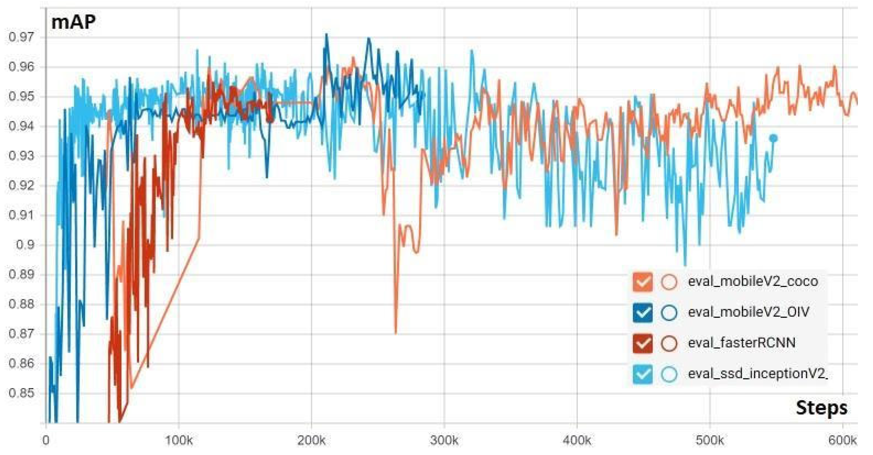
In Figure 2, the mean accuracy precision of all trained models using Pascal VOC metrics is presented. One can notice that the highest mAP is obtained for the SSD MobileNetV2 model pre-trained on the OID dataset. The SSD MobileNetV2 trained on the COCO database [40] is less accurate, although the architecture is similar to the one with best results and the parameter tuning is the same. This might happen because unlike the SSD MobileNetV2 model pre-trained on OID, the weights of the pre-trained model on COCO are frozen at the bottom layers, while the weights at the top layers, where the representative features are learned, are unfrozen in order to be updated according to the TrashNet dataset. The Inception-based SSD and Faster R-CNN model obtained mAP scores over 91%.

In Figure 3, the recall of all trained models is evaluated. As in the case of mAP, the model with the best results in terms of recall is the SSD MobileNetV2 pre-trained on the COCO dataset, followed by Faster R-CNN and Inception V2.

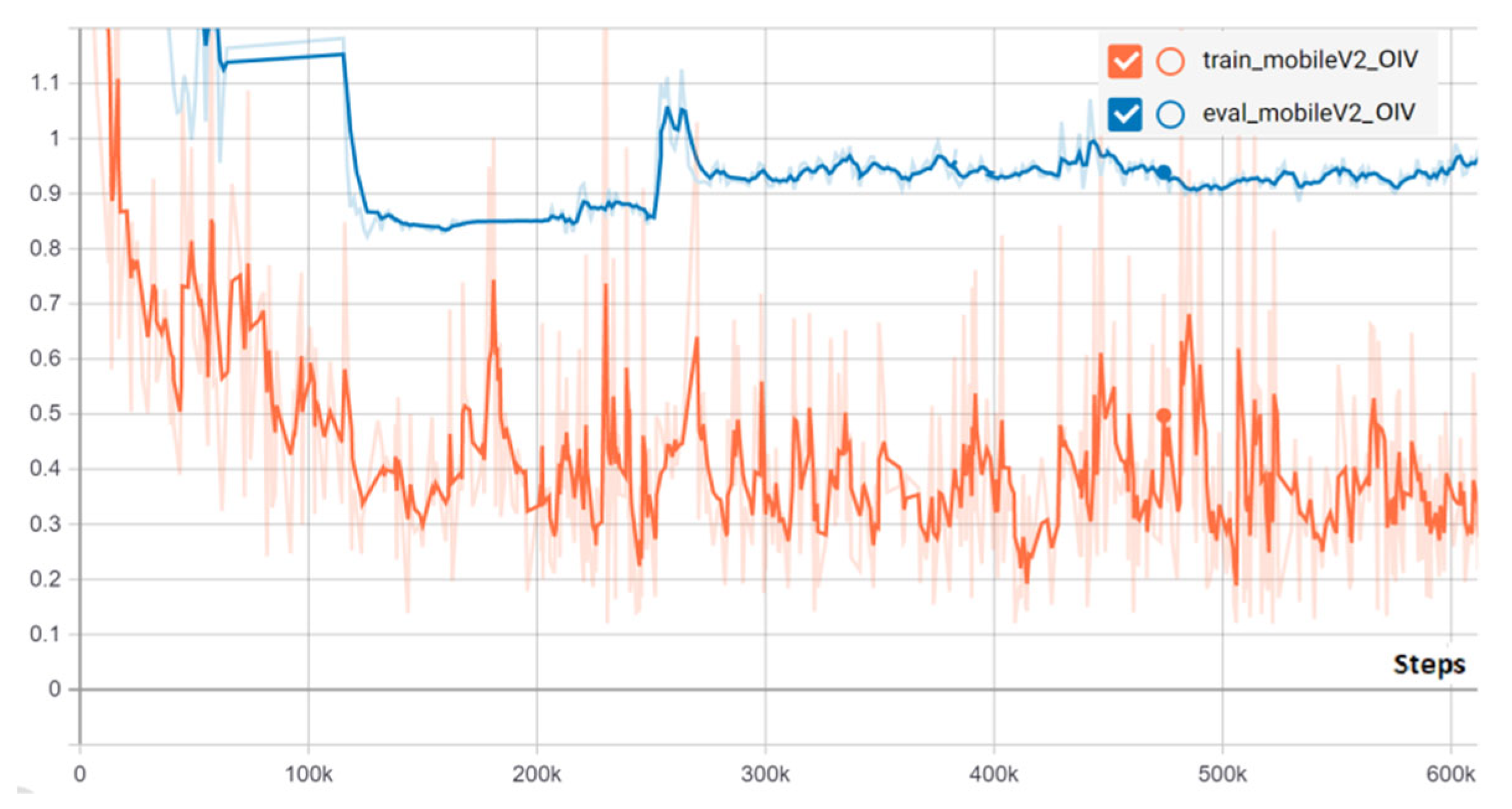
In order to check the models against overfitting, the training and evaluation losses during the entire training have been taken into account. In Figure 4, the classification loss of the most accurate model, the SSD MobileNetV2 network pre-trained on OID V4, is presented during training and evaluation. One can observe that the validation and training losses converge on the same graph, meaning that the CNN manages to generalize well and the images in the training set are accurately detected. The evaluation loss converges to a minimal value around 0.75 after 200 k steps. Due to the fact that the learning rate has been adjusted manually at some checkpoints, there are some sharp increases in the evaluation loss but returns to the prior variation when the changes are undone and meta-parameters are better adjusted. The training and evaluation errors decrease fast during the first part of training (50 k steps). After 50 k steps, the losses decrease on a smoother slope until 150 k steps. From that point on, the classification loss starts to converge until 220 k, when the model begins to overfit (the training loss fluctuates around 0.4, while the validation loss increases). The same evolution has been observed for other models. In order to avoid overfitting, the inference graph of the model has been generated from the checkpoint created at the 203 k step, when the network starts to lose its ability to generalize.

In Figure 5, the localization loss of the SSD MobileNetV2 network pre-trained on OID V4 over time is presented. The validation and training losses follow the same pattern and the error converges after 100 k steps to an average value of 0.04 mm. Just like the classification loss, the same evolution can be observed for other models. The localization loss for training and validation is very small, thus it is not taken into account when evaluating the ability to generalize of the model.

In Figure 6, the learning rates during training are presented. For two of the models, the training starts with a value of 0.004 and decreases until reaching 0.00001 (1 × 10⁻⁵), switching from an exponential to a step decrease. The other two models start from a lower value of 0.0004 until reaching 1 × 10⁻⁵.

In Figure 7, the classification losses of the architectures used in this research are presented. The lowest classification loss comes from the Faster R-CNN network, while the highest is from the SSD Inception V2 model.

3.3. Confusion Matrix

In order to follow the distribution of the true positive, false positive, true negative, and false negative detections per each class, the confusion matrix has been generated. Although the evaluation of the confusion matrix is a little bit different from the COCO and PASCAL VOC metrics, the results are useful to determine the confusion between classes. The confusion matrix for SSD-MobileNetV2 and Faster R-CNN–Inception-ResNet, respectively, are presented in

Table 1. SSD-MobileNetV2 Confusion matrix.

	Glass	Metal	Plastic	Paper	Cardboard	No Detection
Glass	96.23	1.89	0.00	1.89	0.00	0.00
Metal	4.71	90.59	1.18	1.18	0.00	2.35
Plastic	3.03	3.03	92.93	1.01	0.00	0.00
Paper	0.00	1.61	0.00	96.77	0.00	1.61
Cardboard	1.25	1.25	0.00	6.25	87.50	3.75

and

Table 2. Faster R-CNN–Inception-ResNet Confusion matrix.

	Glass	Metal	Plastic	Paper	Cardboard	No Detection
Glass	97.17	2.83	0.00	0.00	0.00	0.00
Metal	8.24	89.41	2.35	0.00	0.00	0.00
Plastic	6.06	2.02	91.92	0.00	0.00	0.00
Paper	0.00	1.61	1.61	93.55	0.00	3.23
Cardboard	0.00	3.75	0.00	10.00	83.75	2.50

. The network with the best performances, according to the confusion matrix, is the SSD-MobileNetV2, followed by Faster R-CNN–Inception-ResNet. The classes with the highest average score for our models were “glass” and “paper”. There are two important aspects that allowed such a good prediction: low variance and large dataset, with the first being the most important. The training dataset plays an important role when learning high-level attributes, but the variance was essential when it came to emphasizing key features. This can be observed as the “glass” class is not the biggest in the training dataset, being outclassed by “paper”. The “paper” class did not manage to generalize as well as “glass” for some networks, although it has the largest share of the dataset. Another thing to notice from the confusion matrices is that metal and plastic are most mistaken with glass. In addition, plastic is confused with metal, while cardboard is mistaken for paper by an average of 8%. This is not uncommon for object detectors because these classes share many similar characteristics (shape, dimensions, color, etc.)

4. Discussion

From

Table 3. Evaluation of fine-tuning object detectors on Pascal VOC metrics.

CNN Model	Precision [%]	Recall [%]	Steps	F1 Score [%]
SSD + MobileNetV2 + COCO	96.09	95.76	500 k	95.92
SSD + Inception V2 + COCO	96.69	94.79	500 k	95.73
SSD + MobileNetV2 + OID V4	97.63	94.39	300 k	95.98
Faster R-CNN + Inception V4 + OID V4	95.76	94.41	300 k	95.08

, it results that the model which achieved the highest accuracy and recall using the PASCAL VOC metrics was SSD+MobileNetV2 pre-trained on OID version 4. There is room for further improvement for this network by using different optimizers like Adam, Adadelta, or Nadam. It is interesting to notice that all the trained object detectors had a precision and F1 score over 95% with our hyper-parameter setting.

For SSD MobileNetV2 pre-trained on OID V4, the mean average precision for each class is evaluated. The highest accuracy is achieved for the glass and metal objects (

Table 4. Best model evaluation for our TrashNet classes.

Class	Accuracy [%]
Cardboard	97.5
Glass	98.33
Metal	98.28
Paper	98.18
Plastic	95.95

).

Furthermore, our best model performances are compared with the results obtained by other CNNs trained on the TrashNet dataset. The comparative evaluation from

Table 5. Evaluation with other trained or fine-tuned model on the TrashNet dataset.

CNN Model	Accuracy/mAP [%]	Object Detector	Fine-Tuning	Optimizer
SSD (MobileNetV2-OID V4)	97.63	Yes	OID V4	RMSProp
MobileNetV2	88	No	ImageNet
Faster R-CNN (Inception V2) [7]	81.6	Yes	COCO
VGG-16 [6]	88.42	No	ImageNet
ResNet50 [9]	87	No	No
RecycleNetV4 [8]	81	No	No	Adam
DenseNet121 [8]	95	No	ImageNet	Adam, SGD
Inception-ResNetV2 [8]	87	No	ImageNet	Adam, SGD

takes into account the accuracy/mAP, optimizers, and whether the models share an object detector architecture or if the networks have been fine-tuned. In terms of object detector, our best model has the highest precision, recall, and F1 score by far and obtained better results than other CNN architectures. Although the object detector architecture is more complex than an Image Classification CNN and the accuracy is measured in a different manner, all the models used in this research obtained better results than these classifiers.

It is worth mentioning that there are differences between the evaluation of Object Detectors (OD) and image classifiers (IC). In our research, we considered that the precision or the F1-Score of OD are tools of measuring the accuracy of the model, although the accuracy parameter of the IC is calculated slightly different. This is why in Table 5 there is a value named “Accuracy/mAP”. Accuracy is used to evaluate the IC and mAP for OD, but both provide insights on the performances of the models. In the same table, in column four, it is mentioned which network is the Object Detector. The reason behind choosing to measure two different types of CNN is because there is only one state-of-the-art paper that used OD for waste detection, with performances well below our results. Moreover, the IC models that have been trained on TrashNet only present the accuracy and loss, not mentioning the precision, recall, or F1-score. Therefore, taking into account that all the models in Table 5, whether they are OD or IC, are trained against the TrashNet dataset, the results provide useful insights on the performances obtained by our network.

Furthermore, in order to evaluate the generalization of our models outside the TrashNet dataset with real-time images, at the inference time, a custom small set of images has been created, consisting of 25 images of plastic and glass bottles which are completely different from the ones the model has been trained with and tested/validated against. The same evaluation has been performed in our first paper regarding municipal waste sorting using CNN [6]. Due to the fact that the detection of bottles in municipal waste is a process that involves identification of objects that have different degrees of deformation, shapes, position, and transparency, this small set of images has been taken into account for testing at the inference time. While bottles are the most common object in municipal waste, our small set consists of plastic and glass bottles.

Figure 8 presents the main case study detections successfully performed. The plastic and glass bottles in the image are placed in different positions (including bottom up), are partially obstructed, deformed, with different shapes, etc.

The evaluation at inference time has been made on our custom dataset, switching the resolution from 300 × 300 to 500 × 500. The 500 × 500 resolution is needed in order to detect small size bottles and cans. The average confidence reached 75.54%, but an object (one plastic bottle) has been misclassified as a can, although the localization was accurate (

Table 6. Evaluation on our waste test dataset at inference time.

Model	Average Confidence Custom Dataset
MobileNetV2 + SSD + OIDV4 + TrashNet	72.8
Faster R-CNN	39.83
MobileNet	27.06
MobileNetV2 + SSD + COCO + VOC	78.13
MobileNetV2 + SSD + COCO	42.31
Inception V2 + SSD + COCO	59.1

). Another thing to note is that the model with the highest average confidence, MobileNetV2 + SSD + COCO + VOC, does not distinguish between recycling waste and only can detect bottles, whether plastic or glass.

This paper focuses on the detection of one waste per each image, but object identification for different degrees of clustering has also been tested, obtaining promising results as well. Although the clutter scenario was not the main focus in this research, the preliminary results will be used for further enhancements of CNN models. For this scenario, the main types of objects encountered during waste sorting have been considered, that is: plastic, glass, and metal. In Figure 9, waste identification for a clutter scenario is presented, considering detections with a confidence score higher than the 50% threshold defined at the inference time. As expected, there are objects that the model has not been able to localize and classify, or the confidence score was lower than 50%. This is quite common for CNN models trained with one object in an image (e.g., TrashNet), instead of multiple objects. The model is biased towards recognizing fewer objects or detecting all the objects in the images as part of the same class and bounding box. Another drawback in clutter scenarios for CNN models trained on the TrashNet dataset is that there is a high aspect ratio between object size and image size, with objects filling a large portion of the image. In order to deal with these outcomes in the future, the TrashNet dataset will be further augmented with images that contain more objects with different sizes of the same class.

The small size of the TrashNet dataset affects the performances of the CNN models. In order to overcome this drawback, data augmentation, transfer learning, and fine-tuning have been used among other techniques.

The model with the best results has a high confidence score when detecting medium and large waste at the inference time but the accuracy drops when handling small objects. When using Faster R-CNN, there is a slight improvement in detecting small objects, but the speed cost is three times higher for a real-time application. To solve this issue, the mobile robot system takes pictures at different distances from the ground. We have noticed that by reducing the distance between objects and camera with 5–10 cm, small waste can be detected.

Another important issue to note is that it is (more) difficult to detect waste that is placed in uncommon positions (including bottom up), or is partially obstructed, deformed, with different shapes, translucent, etc. The confidence score at the inference time in this scenario is much lower than usual detections even lower than the 0.5 threshold. For example, the evaluation outside TrashNet, on a small dataset of uncommon waste images, led to an average confidence of only 75.54%.

The detection at the inference time has been reduced from 0.5 to 9 FPS for SSD architecture and from 0.2 to 4FPS for Faster R-CNN on a Raspberry 3+ board. The improvement of the detection time has been obtained using an extra USB neural network processor from Intel with asynchronous threading. At inference time, the asynchronous API running on the Neural Network USB can improve the overall frame rate of the application. While the accelerator is busy with the inference, the application can continue doing things on the host rather than wait for the inference to complete.

5. Conclusions and Future Work

This paper presents an extensive and in-depth study of convolutional neural network object detectors applied to municipal waste identification. The main objective was to increase the capabilities for some of these pre-trained models. The performance of the CNN object detector is determined, among others, by data augmentation, CNN model, number of images in training/testing dataset, loss optimization, hyper-parameters adjusting, evaluation metrics, transfer learning, fine-tuning, etc. Thus, in order to develop an accurate and real-time architecture, a complex set of actions has been carried out in this research.

The model which achieved the highest accuracy and recall was SSD + MobileNetV2 pre-trained on OID version 4. The performances of this network are compared with the results obtained by other CNNs trained on the TrashNet dataset. In terms of object detectors, our fine-tuned model obtained the highest precision, recall, and F1 score and obtained better results than other CNN Image Classifiers. Although the object detector architecture is more complex than a CNN for classification and the accuracy is measured in a different manner, all the models used in this research obtained better results. There is room for further improvement for this network by using different optimizers like Adam, Adadelta, or Nadam. It is interesting to notice that all the trained object detectors have shown accuracies over 90%, when using the proposed hyper-parameter setting.

In addition to the current work on the TrashNet dataset, annotations for each class are added in order to train the SSD and Faster R-CNN convolutional neural networks.

Most of the CNNs used, for waste sorting output, only the presence and classification of the trash in the picture. Due to the fact that municipal waste usually contains different waste types, an object detector has been used here in order to add localization to our detections.

In order to evaluate the generalization of our models at inference time, 25 images have been taken in laboratory conditions and the average confidence is 10% higher than the results obtained by other models. The paper focuses on the detection of one waste object per each image, but object identification for different degrees of clustering has also been tested, obtaining promising results as well.

Another important thing to note is that detection at the inference time has been reduced to 9 FPS for SSD architecture and to 4FPS for Faster R-CNN on a Raspberry 3 + board. The improvement of the detection time has been obtained using asynchronous threading and one additional neural network processor from Intel.

The model obtained during this research will be further developed so that to determine the municipal waste size and camera–object distance. The practical interest and goal is to allow the mobile robotic system to adjust the gripper stroke and position according to the detected objects. Finding the most appropriate location of the camera on the mobile robotic system will also be a further issue.