Featured Application
Precise control of actuators for transportation, automotive, health equipment…
Abstract
Thanks to their integrability and good electromechanical conversion abilities, piezoelectric actuators are a good choice for many actuation applications. However, these elements feature a frequency-dependent hysteresis response that may yield complex control implementation. The purpose of this paper is to provide the extension of a simple hysteresis model based on a system-level approach linking the strain derivative to the driving voltage derivative and taking into account the dynamic behavior of the hysteretic response of the actuator. The proposed enhancement consists of transient and harmonic regimes, allowing to extend the quasi-static model to dynamic behavior with any frequency. In particular, initial strain shift arising from stabilization and accommodation effects as well as frequency-dependent hysteresis shape are considered. The inclusion of the system dynamics in the model is obtained thanks to fractional derivatives and associated fractional transfer functions, allowing the consideration of the full actuator history as well as a fine tuning of the system dynamics over a wide frequency band. Finally, a numerical example of linearized control through compensation loop is provided, demonstrating the interest in the proposed approach for providing a computationally-efficient, simple yet efficient way for finely predicting the actuator response and thus designing appropriate controllers.
1. Introduction
Thanks to their high integration potential and energy conversion abilities, piezoelectric materials have been of rising interest over the last decades for application in actuation systems [1,2], such as medical probes [3], inkjet devices [4], or car injectors to name just a few examples. However, when actuated at high electric field, such actuators exhibit nonlinear hysteretic effects that may compromise their correct operation. Therefore, properly designing actuators and their associated control system necessitates good understanding and model of such a hysteresis response.
Many hysteresis models are available in the literature [5], mainly for magnetic devices but with possible extension to piezoelectric systems, which can be possibly divided into two kinds of approaches. The first one consists in numerical models, where hysteresis is constructed from many elementary units, called “hysterons”, that are combined together to shape the global actuator’s hysteresis response. Such approaches include the well-known Preisach model [6,7] along with its derivatives such as Krasnosel’Skii–Pokrovskii (KP) technique [8,9], as well as Maxwell–Slip methods and associated dry friction models [10,11]. Usually based on phenomenological approach, such models are effective in finely relating the piezoactuator’s behavior (including minor loops for instance), but are computationally and memory-intensive, therefore preventing their use in lightweight embedded systems. On the other hands, mathematical techniques, based on explicit or implicit formulations, offer hysteresis models with reduced parameter sets and possibly physical interpretation of their construction. This class includes Jiles–Atherton [12,13], Bouc–Wen [14,15], or Duhem [16,17] approaches for instance. However, proper parameter identification as well as stability and faithful representation of particular hysteretic behaviors may raise some issues when considering these techniques.
However, most of the previous models, at least in their initial formulations, where dedicated to quasi-static regime and did not included transient and harmonic behaviors of the actuators, which can however yield significant changes in the electromechanical response. Therefore, works aiming at enhancing such models by including time-dependent components have been proposed in order to provide more accurate representations of hysteretic behavior of piezoelectric or magnetic elements. This includes, for instance, modification of the Bouc–Wen [18], Jiles–Atherton [19], or dry friction [20] approaches, but also numerical techniques such as Preisach approaches [21]. In addition to dynamical effects such as creep or losses (potentially with nonfractional terms [22,23,24,25]), transient stage can also be related to quasi-static regime, for instance through, stabilization and accommodation that relate the partial repolarization due to irreversible polarization process that occurs in ferroelectric materials [26].
In that purpose, this paper proposes an enhancement of a simple mathematical approach inspired by the butterfly loop of piezoelectric materials previously introduced by the authors [27]. Compared to previously exposed models, this approach provides a simple and compact formulation of the hysteretic operator, allowing lightweight implementation with respect to hysteron-based models and part of mathematically-based ones, as well as efficient hysteretic behavior representation including for instance minor loops. This model is besides mainly dedicated to devices while the large majority of other approaches target material characteristics. However, this model, considering the coefficient relating the derivative of the strain with respect to the input voltage derivative, has so far been developed for quasi-static regime without any inclusion of dynamic effects directly within the model (hybrid approach was proposed in [28]). The reported study therefore proposes to directly include in the model relaxation effects as well as repolarization process for providing a generalized method allowing faithful response prediction as driving voltage frequency is varying and/or waveforms get more complex than a pure sine wave. The paper is decomposed as follows. Section 2, after recalling the original model basics, describes the proposed model refinement that takes into account both transient and harmonic effects. Then, Section 3 aims at validating this approach by comparing with experimental measurements performed on a stack actuator. As an example of application, Section 4 provides a numerical implementation of the present model in a compensation loop for precise position control, with the actuator modeled using a previously experimentally validated approach based on hybridization of the quasi-static model with Bouc–Wen approach and filtering [28]. Finally, Section 5 aims at recalling the main points of the paper and concludes about the model validity and potentials.
2. Model Principles
Based on the original model exposed in [27], this section aims at investigating and including transient and harmonic effects in order to relate the actuator behavior for more general excitation cases (waveform, frequency…).
2.1. System-Level Model Basics
The principles of the original hysteresis model for piezoelectric actuators lie in considering the coefficient linking the strain derivative to the voltage derivative as
Obviously, if is a constant, linear relationship holds. However, introducing voltage dependency in and inducing a butterfly shape of this coefficient as a function of the voltage leads to hysteresis in the voltage-strain plane. Specifically, this butterfly form is achieved by applying an effective voltage that equals the driving voltage V minus a memory voltage , set to the driving voltage value when the later reaches a local extremum, or equivalently when its derivative cancels. The coefficient is then obtained through a constant value , relating the linear part of the actuator, and a hysteretic part achieved through a predefined mathematical function h:
Note that the choice of the mathematical function allows obtaining different hysteresis shapes. Specifically, considering the absolute effective voltage in the function yields a symmetric hysteretic behavior, which will be assumed all along this study. Moreover, excluding the linear part from the hysteretic one represented by h leads to the required property for properly relating the small signal behavior. Considering the simple case of linear function such as as an example yields plots depicted in Figure 1, where the driving voltage is a unipolar shifted sine wave. As the driving voltage and memory voltage are zero (position (1)), the increase in the driving voltage to position (2) also yields a linear increase of the coefficient , so that the strain S evolves in a quadratic way. Once in position (2), corresponding to a driving voltage maximum position, the memory voltage is set to this maximal value, so that and goes back to (position (3)). Then, the driving voltage decreases, leading to an increase of (as ) and thus of , until position (4) where the driving voltage reaches a minimum value (actually 0 V in this example) to which is set , as in position (1) where .
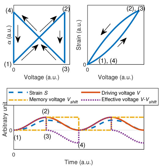
Figure 1.
Original model principle (a.u. refers to “arbitrary units”).
Therefore, this approach provides a quite simple and computationally efficient modeling method, as it only requires a few parameters (typically 1 for the low-field behavior——and 1–2 for the function h) and only one memory () while relating quite well the quasi-static behavior of actuators under various cases [27]. It also provides versatility and adaptivity as the function h can be any function (so that the strain variation is not necessarily quadratic), such as exponential or even Gaussian to get closer to material hysteresis loop [27]. One can note that in the particular case of linear function, the method is quite close to a differential form of Rayleigh hysteresis model [29], but this differential approach permits avoiding issues that arise in unipolar driving when considering the regular Rayleigh approach [30,31].
It has to be recalled here that the model targeting applicative aspects, it mainly aims at relating actuator behaviors under lower excitation magnitude compared to the case of material characterization. In other words, it is considered that compared to the full hysteretic/butterfly shape of the material, only minor material loops are under consideration. Therefore, it is assumed that no significant domain switching occurs for instance. In addition, working quantities in that high-level system view consist in strain and voltage instead of (potentially local) strain and electric field, and global average response of the whole device is under consideration. However, even under these moderate excitations, the actuator still exhibits significant hysteresis behavior.
2.2. Dynamic Effects—Electromechanical Transient Regime and Harmonic Relaxation
However, polarization mechanisms in ferroelectrics, at the origin of piezoelectricity, show time-dependent effects that are not related by the original model described above. Particular relaxation-like phenomena may yield effects such as stabilization and accommodation, creep, or change in the hysteresis loop with the frequency for instance. This study aims at enriching the previously exposed approach by including dynamical effects. In particular, two phenomena will be under focus. First, transient regime, resulting from depolarization for instance and yielding bias in strain even at rest (zero or constant applied voltage) or with time constants not directly related to the driving voltage frequency, will be under consideration. Such an effect can be seen as a change in the initial condition of the actuator. Therefore, during the first cycles upon the voltage application, a drift in the strain response may be observed, which is not related by the initial model exposed in Section 2.1. This effect can physically be partly explained by irreversible polarization and domain rearrangement. Additionally to this transient regime, frequency-dependent behavior can be observed [23], with the hysteresis shape and thus strain response changing as the voltage changes in frequency (but not in magnitude). The strategy adopted in the present study consists in treating such behaviors as particular relaxation phenomena. Furthermore, as these effects may be related to the electrical polarization state of the material, it will be assumed that these relaxations are applied to the driving voltage only (Figure 2).

Figure 2.
Global model schematics.
These transient and harmonic effects are besides related to the whole history of the actuator. Therefore, these relaxation-related effects cannot be taken into account as a classical, Debye-like relaxation model. Instead, non-integer (i.e., fractional) derivatives are good tools for relating these particular features. Indeed, such operators take into account the whole history, with an unlimited memory, of signals and are therefore well adapted to ferroelectrics. On a physical aspect, they are between energy storage terms (potential or kinetic-i.e., zero and second derivation orders of typical quantities such as strain or voltage for instance) and pure losses (first derivation order of typical quantities), therefore allowing taking into account complex phenomena that occur at the material or system level. An example of such an approach is the well-known Cole–Cole relaxation model in dielectrics [32,33], that is, however, classically only considered in the frequency domain (and without hysteresis as well). It could also be noted that, compared to the present approach, the Cole–Cole representation assesses the material behavior at low-field excitation (dielectric spectroscopy for instance), and cannot represent the hysteretic behavior at a system-level as the presently proposed model.
Mathematically, fractional derivatives arise from pseudo-differential operators, and correspond to the fact that, to obtain a classical first-order derivation, a n-fractional derivative operator (with n the possibly non-integer derivation order) has to be applied n times. For example, for , the fractional derivation operator should be applied three times to obtain the first-order derivative of a function f:
with ∘ the composition operator. Consistently with Laplace and Fourier transforms, these fractional operators in the time-domain (as physical systems are ruled by—potentially non-integer—partial differential equations in time-domain) yield a multiplication by and (respectively, in Laplace and Fourier spaces), with s the Laplace variable, the angular frequency and j the unit imaginary number. As an illustration, Figure 3 and Figure 4 show the frequency response and transfer characteristics of the fractional order unit relaxor H defined in the Laplace domain as:
where s is recalled as the Laplace variable and n is the fractional order (). and , respectively, denote the input and output signals of the system represented by the transfer function . These illustrative results have been obtained using the FOMCON (Fractional-order Modeling and Control - version 1.22.0.0, Tallinn University of Technology, Tallinn, Estonia) toolbox for MATLAB® (version R2020a, Mathworks, MA, USA) developed by Tepljakov et al. [34,35]. Therefore, it can be seen from Figure 3 that the frequency response can be finely tuned both in terms of magnitude response and phase, allowing changing the attenuation slope and bandwidth in a precise way. Phase tuning through the fractional order n also permits shaping differently the elliptical input-output characteristics and its frequency behavior as shown in Figure 4. Moreover, a remarkable property when considering unipolar input (Figure 4b) is the ability of relating an almost constant shift after a transient stage, while the entire derivative order yields offsets that significantly change as the frequency increases. Finally, the possibility of finely controlling the system dynamics can also be observed from the step response depicted in Figure 5, showing that low fractional order expands the settling time and thus well relates long-term phenomena.
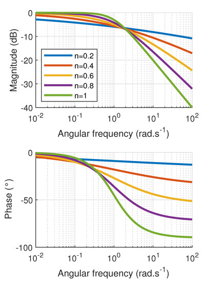
Figure 3.
Frequency response of fractional order unit relaxors (n is the fractional order).
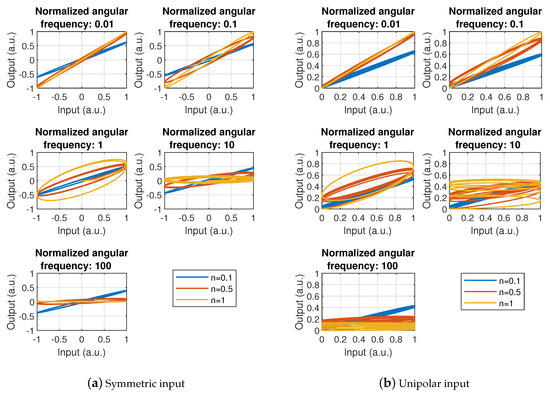
Figure 4.
Input (“”)-output (“”) characteristics of fractional order unit relaxors (n is the fractional order) at several frequencies (a.u. refers to “arbitrary units”).
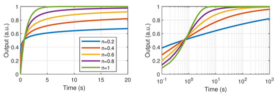
Figure 5.
Step responses of fractional order unit relaxors (n is the fractional order). (Left) linear time scale; (Right) logarithmic time scale (a.u. refers to “arbitrary units”; “Input” and “Output”, respectively, refer to the input and output signal of the system represented by the transfer function (i.e., and ).
Therefore, in order to take into account transient and harmonic effects into the static model and according to Figure 2, the driving voltage V is changed into an equivalent static model input voltage that is obtained after two filtering processes: one representing the transient effect whose transfer function is denoted and the other harmonic phenomena with an associated transfer function . This, therefore, yields in the Laplace domain:
with and , respectively, defined as
with and () the time constant and fractional order associated to each effect, respectively. Obviously, as the transient effect is expected to have a response spanning a wider time period compared to harmonic losses and conversion, one can expect that for relatively small value of s and with .
Alternatively, instead of computing the voltage response in Laplace domain to go back in time domain (with time variable t) for applying the hysteresis model, it is possible to obtain the equivalent voltage by convolution of the impulse responses and , respectively associated with and :
where ∗ is the convolution operator, and and are defined as [36]
with the Mittag–Leffler function:
3. Experimental Validation
3.1. Set-Up and Model Identification
This section details an evaluation of the model performance considering measurements performed on an experimental apparatus. As a system-oriented approach, the objective of this experimental validation is to asses to what extent the model provides a flexible tool to be implemented in a wide variety of control systems for instance.
In order to experimentally investigate the validity of the proposed model, a piezoelectric stack actuator (PICMA® P-888.51 from PI™ Ceramic GmbH, Lederhose, Germany, with an internal capacitance of 6 F and 0–100 V unipolar driving voltage) has been considered. The actuator, that is left in stress-free conditions, is driven by a dSPACE™, Inc, Paderborn, Germany, DS2003/DS2102 acquisition/control system through an amplifying module (PI™ Ceramic GmbH, Lederhose, Germany, E-503). Strain is monitored using a 120.3 strain gauge (BQ120-3CA, Donghua Testing Technology, Jingjiang, China) with a sensitivity of 1.085 mV connected to a signal conditioning module (Donghua Testing Technology, Jingjiang, China, DH 3840). Finally, an oscilloscope (Tektronix™, OR, États-Unis, TDS 1002) is used for additional monitoring of actuator driving voltage. Experimental set-up schematic is depicted in Figure 6.
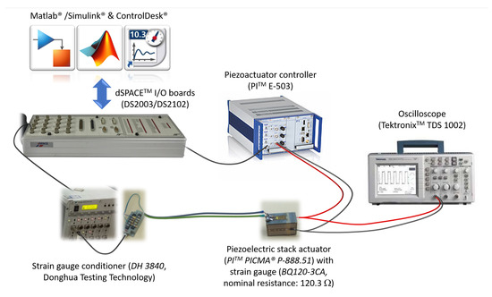
Figure 6.
Experimental set-up.
Experiments consisted in varying applied voltage magnitude (50 and 100 V) and frequency (1, 5, 10, 20, and 40 Hz). Exponential function has been considered for the quasi-static model:
as it relates the hysteresis behavior of the considered actuator with better accuracy than the linear model [27]. In Equation (10), is the maximal variation of the strain derivative-voltage derivative coefficient, and refers to the voltage coefficient allowing the control of the saturation occurrence of the function h. Identification procedure first consisted in characterizing static model parameters (, , and ) by considering steady state at low frequency (1 Hz). More precisely, the procedure consisted in identifying these parameters through the experimentally evaluated value of , as depicted in Figure 7. It can be noted that the parameter for has been found to 6 V, which is quite far from the manufacturer’s datasheet (8.33 V). This is explained by the fact that transient effect still arises at this frequency. Hence, next procedures will need to include a refinement for .
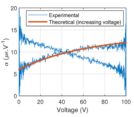
Figure 7.
Low frequency characterization. Theoretical plot has been obtained using Equation (10).
Then, still at the same frequency, transient response (strain shift) was used for finding the values of transient regime fractional derivative order () and time constant (), as well as refining (Figure 8). Finally, high frequency excitation (5–40 Hz) permitted extracting the values of the harmonic regime fractional derivative order () and time constant (). Model parameters are listed in Table 1. It is interesting to note that the best value found for the harmonic regime fractional derivation order, , is greater than 1, meaning that the associated behavior is between losses and kinetic energy, while one may expect it to be between potential energy and losses (i.e., ). However, the fractional derivation order associated to transient regime follows this expectation quite well, with a quite small value well denoting a slowly varying process with frequency. It could also be noted that the use of the strain derivative-voltage derivative coefficient in the characterization procedure may yield some inaccuracy in the identification procedure as a numerical differentiation is performed (in Figure 7 and Figure 8 a 10-point smoothing is applied, which, however, does not yield a significant distortion, as the sampling frequency of 1 ms is 1000 times the driving signal frequency). However, the fact that the theoretical results match these experimental data over a wide voltage range implies a quite high confidence in the found parameter values.
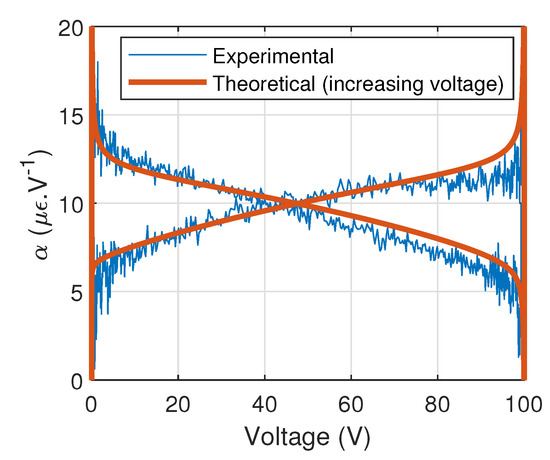
Figure 8.
Low-frequency characterization taking into account transient stage. Theoretical plot has been obtained using Equation (10).

Table 1.
Model parameters.
3.2. Results
3.2.1. Harmonic Excitation at Different Amplitudes and Frequencies
First experimental measurement set consisted in applying a 50 or 100 V driving voltage magnitude at varying frequencies. Maximal frequency is limited by the maximal output current of the E-503 amplifier [37], yielding a limit approximately equal to 55 Hz for the considered actuator and maximal driving voltage. Therefore, experimental driving frequency has been limited to 40 Hz to ensure that no distortion occurs.
Experimental results, along with model predictions (where the fractional derivatives were obtained using FOMCON toolbox [34,35]), are depicted in Figure 9. Therefore, results show very good agreement between experimentally measured responses and predicted ones. In particular, the model shows good abilities in relating the change in the hysteresis loop, as also illustrated by Figure 10a that depicts the hysteresis loop area, which appears to follow, in the considered frequency range, a rather linear increase. Such an accurate description is enabled by the fractional derivative approach along with its combination with the static model which permits shaping the hysteresis loops as well as its dependence with the driving voltage magnitude.
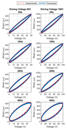
Figure 9.
Experimental results and comparison with model predictions under sine excitation for several driving voltage magnitudes and frequencies.
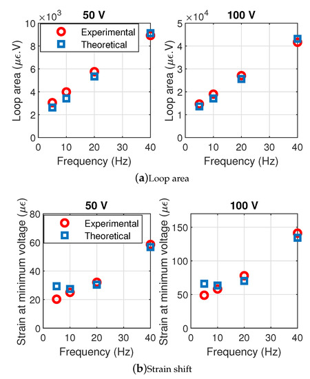
Figure 10.
Experimental and predicted loop areas in steady state and strain shifts.
In addition to this harmonic regime consideration, the transient stage, which yields a bias in the strain response in spite of zero minimal voltage due to accommodation and stabilization effects for instance, is also well related by the proposed approach. This can also be demonstrated by the zero-voltage strain depicted in Figure 10b. Again, this ability of relating transient regime are permitted by the fractional derivative included in the quasi-static hysteresis model; considering a first-order integer derivative would lead to a transient regime that would exhibit too important variations in the strain shift as the frequency is changing.
3.2.2. Varying Voltage Magnitude
In addition to the previously exposed harmonic response, the second experimental investigation aimed at assessing the effect of a non-sinusoidal excitation, by introducing a vanishing envelope to the driving voltage (Figure 11). Considering a center frequency of 1 Hz, results are shown in Figure 12, both in terms of voltage–strain curve and strain time-domain waveforms. Again, good agreement between experimental measurements and model prediction can be observed, with a slight overestimation of the strain when considering the theoretical analysis. Still, the model quite accurately relates the hysteretic effect of the actuator, including minor loops. It can be noted that while the sole quasi-static model would yield minor loops sticking to the main one, the introduction of time-dependent fractional derivatives allows predicting detachment of such minor loops from the main path, as well as smooth strain rate reversal.
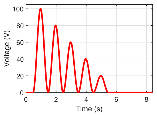
Figure 11.
Experimental driving voltage with varying amplitude.
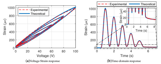
Figure 12.
Experimental and predicted response for varying voltage amplitude.
Nevertheless, one of the major assets of the enhancement provided by this study is the ability to relate well the strain offset that appears. In particular, time-domain waveforms in Figure 12b show that the proposed approach permits assessing the change in such a strain shift as the voltage magnitude decreases. Moreover, it can be noted that, even when the driving voltage keeps zero value, strain continues to decrease (time longer than 5.5 s), which is also very well predicted by the model as shown in the enlargement in Figure 12b.
4. Numerical Example: Application to Linearized Control
Based on the previous model that includes static, transient, and harmonic regimes, it is proposed in this section to illustrate the interest in the exposed approach for providing a mean for efficiently and accurately controlling a piezoelectric actuator with respect to a given strain command. This illustrative example will be numerically evaluated by considering an experimentally validated model of the same actuator used in the previous section and exposed in [28], using a Bouc–Wen model for relating the transient regime and a fourth-order transfer function for the harmonic behavior (Figure 13). Note that compared to the work in [28], the harmonic transfer function has been converted to Laplace domain through bilinear transform as:
with S the actuator output strain and the output of the quasi-static model (made of linear, system-level, and Bouc–Wen blocks). Also, to accommodate with the slight discrepancies between the hybrid model in [28] and actual experimental device, the values of , , and have been marginally changed to 0.2, 32 × 10 s and 2.2 × 10 s, respectively (note that for the transient-related fractional transfer function, this changes the coefficient of the frequency-dependent term from 0.19 s to 0.2 s). All the other parameters are kept the same as per Table 1.
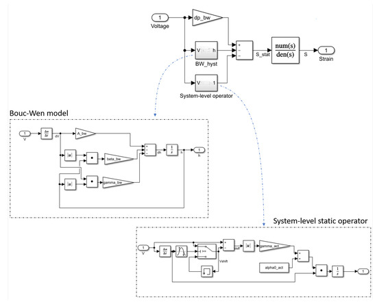
Figure 13.
Considered model of the piezoelectric actuator for the control assessment.
The principles of the proposed control scheme lie in a compensation approach as exposed in [38]. More precisely, based on the model related in this study (Figure 2), the expression of the strain S in the Laplace domain yields:
with the hysteresis operator (defined by the function h and voltage memory , but not including the linear part given by ). Therefore, considering that is the desired output strain, the corresponding required voltage can be found from Equation (12) as
The corresponding implementation for the control is depicted in Figure 14 (the fractional derivative blocks being also part of the FOMCON toolbox [34,35]), along with the actuator model of [28] presented in Figure 13 and a direct control path consisting of the inversion of the sole linear part. Note that compared to Equation (12), model reduction was performed by including the compensation loop before the inverse transient and harmonic functions, and thus removing the associated direct functions before the hysteresis block.
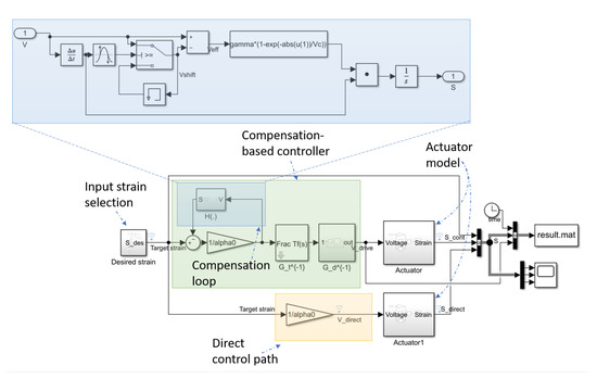
Figure 14.
Schematic of the application example to linearized control.
Figure 15 shows the system response under sine excitation at various frequencies. Therefore, it can be seen that the compensation approach including the proposed model allows significantly limiting the hysteretic response of the actuator and provides a mean of allowing a good and accurate control from a desired strain. Additionally, it can be observed that the proposed approach also addresses well the strain drift, as the strain bias at zero voltage appearing in the direct control case is significantly suppressed when using the compensation technique. Slightly lower and larger strains can be noted however at low and high frequencies respectively, which can however be attributed to slight deviation of the actuator model compared to the real one [28].
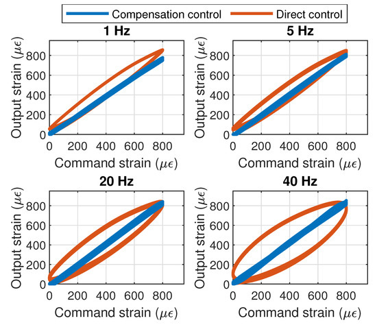
Figure 15.
Control using compensation in sine case.
Moreover, the case of a sine input strain with exponential vanishing magnitude is depicted in Figure 16. In addition to the significant hysteresis reduction including minor loops, such results also show the ability of ensuring that the strain goes back to zero as the command vanishes towards this value, thanks to the inclusion of the fractional transient term. Such characteristics can also be observed on the driving voltage obtained in the compensation approach and depicted in Figure 17, where the strain shift in open loop is efficiently addressed by computed voltages below 0 V.
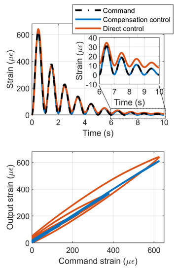
Figure 16.
Control using compensation considering time-dependent magnitude strain command.
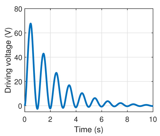
Figure 17.
Control voltage considering time-dependent magnitude strain command.
5. Conclusions
This study reported the enhancement of a system-level hysteresis model for piezoelectric actuators based on voltage-dependent strain derivative/voltage derivative coefficient, and using shift and reversal of a mathematical function, therefore providing a simple yet efficient way for assessing the actuator behavior. While the original model works in quasi-static regime only, this paper extended its applicability to transient and harmonic regimes. To this end, fractional transfer functions applied to the driving voltage were considered. Thanks to their ability of taking into account the whole history of the actuator and their capability of providing finely tunable system dynamics, fractional derivatives have been shown to allow taking into account transient strain shift effects as well as frequency-dependence of the hysteresis shape in harmonic regime, without compromising the model simplicity. Finally, a numerical example of the application of this model to linearized actuator control based on compensation approach was provided. Therefore, it was demonstrated that the model provides a computationally-efficient yet accurate way for describing the behavior of piezoelectric actuators (but with possible extension to any other kind of actuators, e.g., electromagnetic) including transient and harmonic aspects, with potential use in embedded controllers for instance. To further enhance the model applicability, other effects such as loading or temperature dependent behaviors can be considered as potential further works. In particular, regarding the latter aspect (temperature dependence), it is possible to take advantage of the proposed model. As an example, the effect of temperature on polarization (e.g., working near Curie temperature) can be included in the hysteretic operator (strain derivative/voltage derivative coefficient ) while the potential additional losses may be better included in the fractional terms.
Author Contributions
Conceptualization, M.L.; methodology, M.L.; software, M.L. and K.L.; validation, K.L.; formal analysis, M.L.; investigation, K.L.; resources, Z.Y.; data curation, M.L. and K.L.; writing—original draft preparation, M.L.; writing—review and editing, M.L., S.Z. and Z.Y.; visualization, M.L.; supervision, Z.Y., M.L., and S.Z.; project administration, S.Z. and Z.Y.; funding acquisition, Z.Y. and S.Z. All authors have read and agreed to the published version of the manuscript.
Funding
This research was supported by 111 project No. BP0719007.
Conflicts of Interest
The authors declare no conflict of interest.
References
- Lallart, M. (Ed.) Ferroelectrics–Applications; Sciyo/Intech: Rijeka, Croatia, 2011; ISBN 978-953-307-456-6. [Google Scholar]
- Wu, J.; Gao, X.; Chen, J.; Wang, C.-M.; Zhang, S.; Dong, S. Review of high temperature piezoelectric materials, devices, and applications. Acta Phys. Sin. 2018, 67, 207701. [Google Scholar]
- Chorsi, M.T.; Curry, E.J.; Chorsi, H.T.; Das, R.; Baroody, J.; Purohit, P.K.; Ilies, H.; Nguyen, T.D. Piezoelectric Biomaterials for Sensors and Actuators. Adv. Mater. 2019, 31, 1802084. [Google Scholar] [CrossRef] [PubMed]
- Chiatto, M.; Capuano, F.; Coppola, G.; De Luca, L. LEM Characterization of Synthetic Jet Actuators Driven by Piezoelectric Element: A Review. Sensors 2017, 17, 1216. [Google Scholar] [CrossRef] [PubMed]
- Hassani, V.; Tjahjowidodo, T.; Do, T.N. A survey on hysteresis modeling, identification and control. Mech. Syst. Sig. Proc. 2014, 49, 209–233. [Google Scholar] [CrossRef]
- Preisach, F. Uber die magnetische nachwirkung. Z. Phys. 1935, 94, 277–302. [Google Scholar] [CrossRef]
- Song, X.; Duggen, L.; Lassen, B.; Mangeot, C. Modeling and identification of hysteresis with modified Preisach model in piezoelectric actuator. In Proceedings of the 2017 IEEE International Conference on Advanced Intelligent Mechatronics (AIM), Munich, Germany, 3–7 July 2017. [Google Scholar] [CrossRef]
- Krasnosel’Skii, M.A.; Pokrovskii, A.V. Systems with Hysteresis; Springer: Berlin, Germany, 1989. [Google Scholar]
- Qin, Y.; Zhao, X.; Zhou, L. Modeling and Identification of the Rate-Dependent Hysteresis of Piezoelectric Actuator Using a Modified Prandtl-Ishlinskii Model. Micromachines 2017, 8, 114. [Google Scholar] [CrossRef]
- Sebald, G.; Boucher, E.; Guyomar, D. A model based on dry friction for modeling hysteresis in ferroelectric materials. J. Appl. Phys. 2004, 96, 2785–2791. [Google Scholar] [CrossRef]
- Al-Bender, F.; Lampaert, V.; Swevers, J. The generalized Maxwell-slip model: A novel model for friction simulation and compensation. IEEE Trans. Autom. Control 2005, 50, 1883–1887. [Google Scholar] [CrossRef]
- Jiles, D.C.; Atherton, D.L. Theory of the magnetisation process in ferromagnets and its application to the magnetomechanical effect. J. Phys. D Appl. Phys. 1984, 17, 1265–1281. [Google Scholar] [CrossRef]
- Jiles, D.C.; Atherton, D.L. Theory of ferromagnetic hysteresis (invited). J. Phys. D Appl. Phys. 1984, 55, 2115–2120. [Google Scholar] [CrossRef]
- Bouc, R. Forced vibration of mechanical systems with hysteresis. In Proceedings of the Fourth Conference on Nonlinear Oscillation, Prague, Czech Republic, 5–9 September 1967; p. 315. [Google Scholar]
- Wen, Y.K. Method for random vibration of hysteretic systems. J. Eng. Mech. 1976, 102, 249–263. [Google Scholar]
- Duhem, P. Die dauernden aenderungen und die thermodynamik. Z. Phys. Chem. 1897, 22, 543–589. [Google Scholar] [CrossRef]
- Wang, G.; Chen, G. Identification of piezoelectric hysteresis by a novel Duhem model based neural network. Sens. Actuators A Phys. 2017, 264, 282–288. [Google Scholar] [CrossRef]
- Zhu, W.; Rui, X.-T. Hysteresis modeling and displacement control of piezoelectric actuators with the frequency-dependent behavior using a generalized Bouc–Wen model. Precis. Eng. 2016, 43, 299–307. [Google Scholar] [CrossRef]
- Szewczyk, R.; Frydrych, P. Extension of the Jiles–Atherton model for modelling the frequency dependence of magnetic characteristics of amorphous alloy cores for inductive components of electronic devices. Acta Phys. Pol. A 2010, 118, 782–784. [Google Scholar] [CrossRef]
- Ducharne, B.; Guyomar, D.; Sebald, G. Low frequency modelling of hysteresis behaviour and dielectric permittivity in ferroelectric ceramics under electric field. J. Phys. D Appl. Phys. 2007, 40, 551–555. [Google Scholar] [CrossRef]
- Bernard, Y.; Mendes, E.; Bouillault, F. Dynamic hysteresis modeling based on Preisach model. IEEE Trans. Magn. 2002, 38, 885–888. [Google Scholar] [CrossRef]
- Guyomar, D.; Ducharne, B.; Sebald, G. Time fractional derivatives for voltage creep in ferroelectric materials: Theory and experiment. J. Phys. D Appl. Phys. 2008, 41, 3143–3153. [Google Scholar] [CrossRef]
- Ducharne, B.; Zhang, B.; Guyomar, D.; Sebald, G. Fractional derivative operators for modeling piezoceramic polarization behaviors under dynamic mechanical stress excitation. Sens. Actuators A 2013, 189, 74–79. [Google Scholar] [CrossRef]
- Liu, Y.; Shan, J.; Qi, N. Creep modeling and identification for piezoelectric actuators based on fractional-order system. Mechatronics 2013, 23, 840–847. [Google Scholar] [CrossRef]
- Ding, C.; Cao, J.; Chen, Y.Q. Fractional-order model and experimental verification for broadband hysteresis in piezoelectric actuators. Nonlinear Dyn. 2019, 98, 3143–3153. [Google Scholar] [CrossRef]
- Iványi, A. Hysteresis Models in Electromagnetic Computation; Akadémiai Kiadó: Budapest, Hungary, 1997; ISBN 963-05-7416-0. [Google Scholar]
- Lallart, M.; Li, K.; Yang, Z.; Wang, W. System-level modeling of nonlinear hysteretic piezoelectric actuators in quasi-static operations. Mech. Syst. Signal Process. 2019, 116, 985–14996. [Google Scholar] [CrossRef]
- Li, K.; Yang, Z.; Lallart, M.; Zhou, S.; Chen, Y.; Liu, H. Hybrid hysteresis modeling and inverse model compensation of piezoelectric actuators. Smart Mater. Struct. 2019, 28, 115038. [Google Scholar] [CrossRef]
- Lord, R. On the behaviour of iron and steel under the operation of feeble magnetic forces. Philos. Mag. Ser. 1887, 1, 225–248. [Google Scholar]
- Park, J.; Moon, W. Hysteresis compensation of piezoelectric actuators: The modified Rayleigh model. Ultrasonics 2010, 50, 335–339. [Google Scholar] [CrossRef]
- Zhang, M.; Damjanovic, D. A quasi-rayleigh model for modeling hysteresis of piezoelectric actuators. Smart Mater. Struct. 2020, 29, 075012. [Google Scholar] [CrossRef]
- Cole, K.S.; Cole, R.H. Dispersion and Absorption in Dielectrics-I Alternating Current Characteristics. J. Chem. Phys. 1941, 9, 341–352. [Google Scholar] [CrossRef]
- Cole, K.S.; Cole, R.H. Dispersion and Absorption in Dielectrics-II Direct Current Characteristics. J. Chem. Phys. 1942, 10, 98–105. [Google Scholar] [CrossRef]
- Tepljakov, A.; Petlenkov, E.; Belikov, J. FOMCON: A MATLAB toolbox for fractional-order system identification and control. Int. J. Microelectron. Comput. Sci. 2011, 2, 51–62. [Google Scholar]
- Tepljakov, A. FOMCON: Fractional-Order Modeling and Control. 2012. Available online: http://www.fomcon.net/ (accessed on 16 October 2020).
- Petráš, I. Fractional Derivatives, Fractional Integrals, and Fractional Differential Equations in Matlab. In Engineering Education and Research Using MATLAB; Assi, A., Ed.; Intech: London, UK, 2011; pp. 239–264. [Google Scholar]
- PI™ E-503 Piezo Amplifier Module Datasheet. Available online: https://static.piceramic.com/fileadmin/user_upload/physik_instrumente/files/datasheets/E-503-Datasheet.pdf (accessed on 12 August 2020).
- Rakotondrabe, M. Bouc-Wen modeling and inverse multiplicative structure to compensate hysteresis nonlinearity in piezoelectric actuators. IEEE Trans. Autom. Sci. Eng. 2011, 8, 428–431. [Google Scholar] [CrossRef]
Publisher’s Note: MDPI stays neutral with regard to jurisdictional claims in published maps and institutional affiliations. |
© 2020 by the authors. Licensee MDPI, Basel, Switzerland. This article is an open access article distributed under the terms and conditions of the Creative Commons Attribution (CC BY) license (http://creativecommons.org/licenses/by/4.0/).