Multi-Body Dynamics Modeling and Control for Strapdown Inertially Stabilized Platforms Considering Light Base Support Characteristics

Abstract

The dynamics model used for inertially or strapdown inertially stabilized platforms is based on the rotor and motor load, and it either does not consider the stator or it implicitly assumes a fixed stator. It has been determined that vibrations occur in the system when a controller is used in strapdown inertially stabilized platforms with a light base support. As the system is also affected by multi-source disturbances, which are the main factors that affect the control accuracy. For the above two problems, this paper originally establishes a multi-body dynamics model including the controller. The composite controller not only suppresses the vibration successfully, but also greatly improves the disturbance compensation and tracking performance of the strapdown inertially stabilized platforms. Specifically, a modified feedback controller is used to suppress the vibrations analyzed according to the dynamics model. The friction feedforward and residual disturbance observer facilitates the design of compound disturbance compensation on the basis of composite hierarchical anti-disturbance control. To emphasize the advantages of strapdown inertially stabilized platforms, the feedforward controller employs feedforward angular velocity and acceleration. The results of the numerical analysis and experiments indicate that vibrations are successfully suppressed and tracking accuracy and disturbance isolation ability are improved.

1. Introduction

Inertially stabilized platforms (ISPs) are installed on moving carriers, such as aircraft and ships. ISPs provide stable direction for the photoelectric equipment inside the platform in inertial space. They are used extensively in airborne remote sensing, photoelectric detection, target tracking, navigation, and optical communication [1]. Generally, the stable platform is composed of three orthogonal mechanical frames: outer, middle, and inner frames. The photoelectric device and gyroscope sensor are often installed in the inner frame. The gyroscope directly measures the photoelectric equipment inertial angular velocity, and achieves inertial stable imaging by controlling the torque motor rotation in each frame. The platform compensates for the carrier attitude influence, external environment disturbance, and internal disturbance of the system [2]. When the photoelectric equipment operates with a small field of view, the system needs a higher degree of stability accuracy to obtain clearer images. Therefore, designing an effective control method is significant for improving the overall system performance.

Currently, the most commonly used control schemes in research and engineering utilize a gyroscope to calculate the photoelectric equipment angular velocity error in inertial space and to achieve closed-loop feedback control [3,4]. This scheme is simple and effective; however, to achieve high-precision control, feedforward control is also needed in addition to feedback control. The feedforward controller comes from the control command. However, because of the limitation of gyro location, the control command is zero in the process of inertial stabilization, making it difficult to design a feedforward controller. This limitation prevents further system performance improvements. Besides being installed in the inner frame, the gyroscope can also be installed on the platform base to measure its attitude change. The encoder sensor on the motor can be used to achieve the strapdown inertial stabilization with reverse compensation [5,6]. This scheme is directly sensitive to base rotation. It can effectively use the base motion information to construct the feedforward controller and achieve perfect tracking via the reverse motion of each motor. In theory, it can achieve zero-error control performance for some bandwidths [7].

Nevertheless, environmental and mechanical structural factors cause the platform to be disturbed by multi-source disturbances, which include the platform base attitude change, external environment disturbances, and internal system disturbances. Among them, the internal system disturbances, such as nonlinear friction, wire-wound torque, mass unbalance, and model uncertainty, are more complex. In addition, they seriously affect the stability accuracy of the line of sight (LOS).

To deal with these disturbances, a variety of methods have been independently proposed and applied in related fields [8]. These include disturbance observer control (DOBC) [9], active disturbance rejection control (ADRC) [10,11], disturbance accommodation control [12], and nonlinear disturbance observer control (NDOBC) [13]. However, most control methods focus on one type of disturbance or they consider multiple disturbances as an equivalent disturbance. This may lead to conservative disturbance compensation in the presence of multiple disturbances [14,15]. For multi-source disturbances, composite hierarchical anti-disturbance control (CHADC) is an important means to address the above-mentioned problems. The idea is to design multiple loops to compensate for the different types of disturbances, so that high-precision disturbance compensation can be achieved. Furthermore, $H_{\infty }$ control [16], sliding mode control (SMC) [17,18], or adaptive control [19] is integrated with the disturbance compensation method to achieve tracking performance and for disturbance attenuation. The disturbance compensation loop based on CHADC is designed inside the velocity loop; the velocity loop focuses on tracking the performance, and the compensation loop focuses on the disturbance separately [20].

Recently, several researchers have proposed a variety of methods to handle disturbances in IS/SISPs. The traditional design controller method focuses on feedback loops. The proportional integral derivative (PID) control method has been widely used in industrial control systems owing to its simple structure and parameter adjustment capabilities. A SMC has been proposed to achieve a better steady-state accuracy than PID control [21]. As the system is affected by matched and unmatched uncertainties, a modified feedforward-based extended state observer has also been proposed to achieve high tracking performance [22]. Owing to nonlinear factors, such as friction, wire-wound restraint, sensor noise, un-modeled parts, or the varying system parameter, the system stability accuracy cannot be guaranteed by using the velocity loop. To address this problem, a novel discrete-time direct model reference adaptive control based on nonlinear friction compensation has been introduced into the original PI control system [23]. A stable control method based on ADRC and a noise reduction method based on the disturbance observer (DOB) have been proposed to handle the system disturbance and to improve the anti-disturbance capability in a strapdown inertially stabilized platform (SISP) [24].

To achieve better disturbance compensation, the main disturbance needs to be analyzed. Then, an effective control method should be designed on the basis of the model. The primary nonlinear disturbance in the SISP system with a harmonic drive is friction caused by the transmission mechanism relative motion. The traditional friction compensation method measures the relative angular velocity and fits the friction model. The feedback controller contains the negative friction compensation on the basis of the model [25]. The work in [26] adopted a LuGre model-based friction compensation method to design the controller. The disadvantage of this method is the existence of a delay in the sampling period in the control system. As the nonlinear friction torque forms the feedback loop, the instability problem is apparent [27].

In addition to multi-source disturbances, we found that SISP systems supported by light bases will vibrate when using a PI feedback controller only. The vibration of the closed-loop control system seriously affects the performance of the system, and so does adding a disturbance compensation controller or other advanced controllers. Therefore, we need to design a controller to suppress the vibration before disturbance compensation. To suppress the vibration, the model of this system should be analyzed carefully. The conventional system dynamics model employs motor rotor and load only, without considering the stator, or it implicitly assumes a fixed stator. The base of the SISP is connected with the motor stator, and the control system command emerges from the base movement, that is, the motor stator movement, in the inertial space. The control value corresponds to the motor output torque, it acts on the rotor and load, and the reaction torque also acts on the base. The reason for the vibration is that the influence of the light base support and the control on the dynamic characteristics of the whole system is not considered. This is highlighted by the location of the gyroscope in the SISP.

To solve the multi-source disturbance and vibration problem, we first consider the motor stator (platform base), motor rotor, and load as three rigid bodies and establish a multi-body dynamics model by the Euler method, which is commonly used in robotics [28,29]. This model can describe the interaction of the system better. Inspired by CHADC [16] and the triple-step control method [30], this study establishes a composite controller comprising three parts: a modified feedback controller, a compound disturbance compensation controller, and a feedforward controller. The modified feedback controller is designed to suppress the vibration analyzed in the dynamics model. The compound disturbance compensation controller is designed by the friction feedforward method and the residual disturbance observation. On the basis of suppressing the vibration and the composite anti-disturbance control, this study emphasizes the structural advantages of SISP, and further enhances the dynamic performance via the feedforward controller.

In summary, compared with the current state-of-the-art research, the major contributions of this study are as follows.

(a)

To analyze the vibration, the platform base and the motor rotor are treated as an interaction subsystem and the motor rotor and the load are treated as a two-mass-like subsystem. Consequently, this study proposes a multi-body dynamics model including the controller for SISP.

(b)

To suppress the vibration, compensate the multi-source disturbances, and to achieve high performance, the composite controller is designed by three components based on the idea of triple-step control. The proposed method sets the basis for the engineering design of SISPs with a light base support.

The remaining sections of this paper are organized as follows. In Section 2, the dynamics model for SISP is established. In Section 3, the SISP model considering light base support characteristics is analyzed to evaluate the vibration. Section 4 proposes an improved control method that comprises the modified PI feedback controller, the compound disturbance compensation controller, and the feedforward controller. The experimental setup and results are described in Section 5. Finally, Section 6 presents the conclusions of this study.

2. Dynamics Modeling for the SISP

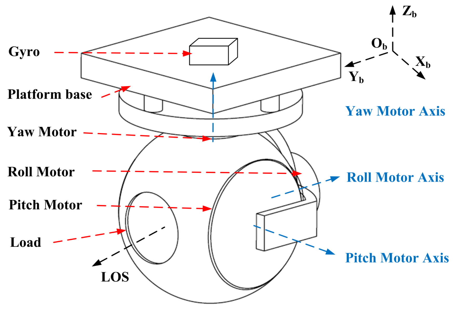
There are many kinds of SISPs according to the application, Figure 1 shows a typical three-axis SISP for the moving base carrier.

Figure 1 shows that the gyroscope mounted on the platform base is used to measure the base inertial angular velocity. The gyroscope generates the command in real-time to make the three motors reverse its motion to stabilize the LOS. The platform consists of three frames: yaw, roll, and pitch. The moment of inertia balance of each frame is typically considered in the ISP/SISP design process; furthermore, each frame uses the same motor, driver, and control method. Thus, this study takes the yaw frame as an example to expand the analysis.

Presently, the model in the ISP/SISP is regarded as a common model of a motor and a load in engineering applications and academic research. However, the traditional model used in the SISP system with light base support is limited by the vibration. A complete SISP system dynamics model comprises the platform base, motor rotor, and load, which are treated as several rigid bodies. To amplify the driver torque in a SISP with a heavy load, a motor with a harmonic drive is used, as shown in Figure 2.

The core of the control system comprises three parts: motor rotor (a), harmonic drive (b), and load (c). Here, the platform base and the motor rotor (a) form an interaction subsystem, while the motor rotor (a) and the load (c) form a two-mass-like subsystem. The harmonic drive (b) mechanism consists of a wave generator, flex spline, and circular spline [31,32]. The motor electromagnetic torque $T_m$ acts on the wave generator in the harmonic drive. The encoder is installed between the motor rotor (a) and the harmonic drive (b). The encoder data represent the relative rotation angle between the motor rotor and stator.

Each part of the system is then modeled and analyzed. The armature voltage balance equation and the electromagnetic torque equation can be described as follows,

$$u_a\left(t\right)-e_a\left(t\right)=L_a{\dot{i}}_a\left(t\right)+R_a{i}_a\left(t\right)$$

(1)

$$K_t{i}_a\left(t\right)=T_m\left(t\right)$$

(2)

where $u_a\left(t\right)$ is the armature voltage, $e_a\left(t\right)$ is the back-EMF, $L_a$ is the armature inductance, $i_a\left(t\right)$ is the armature current, $R_a$ is the armature resistance, and $K_t$ is the electromagnetic torque constant. $T_m\left(t\right)$ is the motor electromagnetic torque acting on the wave generator in the harmonic drive.

The SISP control system typically includes the position, velocity, and current loops. The velocity loop is the most important component; it determines the disturbance isolation capability and the command tracking performance. Because SISP typically operates at a low velocity, the influence of the back-EMF $e_a\left(t\right)$ can be ignored. The DC electric part is a first-order inertial object. On the other hand, the current closed-loop system model is equivalent to a low-pass filter with a high cut-off frequency. Therefore, for the velocity loop, the subsystem from the control voltage $u\left(t\right)$ to the electromagnetic torque $T_m\left(t\right)$ can be regarded as a linear function:

$$K_{a}u\left(t\right)=T_m\left(t\right)$$

(3)

where $u\left(t\right)$ is the control voltage as the input to the current driver and $K_a$ is the coefficient from the control voltage to the electromagnetic torque.

The torque balance equation for the motor rotor can be expressed as follows,

$$T_m\left(t\right)-F_m\left(t\right)=J_m{\ddot{\theta }}_m\left(t\right)+B_m{\dot{\theta }}_m\left(t\right)+T_{wg}\left(t\right)$$

(4)

where $F_m\left(t\right)$ is the total disturbance torque, $J_m$ is the motor rotor equivalent moment of inertia, $B_m$ is the motor rotor equivalent damping coefficient, ${\theta }_m\left(t\right)$ is the motor rotor angle in the inertial space, and $T_{wg}\left(t\right)$ is the wave generator input torque.

The harmonic drive enlarges $T_{wg}\left(t\right)$ by N times and, at the same time, it reduces the angle by N times [33]. The relationship is as follows,

$$N{\theta }_m\left(t\right)={\theta }_m^{{}^{\prime }}\left(t\right)$$

(5)

$$N{T}_{wg}\left(t\right)=T_{fs}\left(t\right)$$

(6)

where $T_{fs}\left(t\right)$ and ${\theta }_m^{{}^{\prime }}\left(t\right)$ are the output torque and the output angle of the flex spline in the harmonic drive, respectively.

The angular deformation in the harmonic drive $\Delta \theta \left(t\right)$ [34] is expressed as follows,

$$\Delta \theta \left(t\right)={\theta }_m^{{}^{\prime }}\left(t\right)-{\theta }_l\left(t\right)$$

(7)

where ${\theta }_l\left(t\right)$ is the load inertial angle.

The transmission compliance acting between $\Delta \theta \left(t\right)$ and $T_{fs}\left(t\right)$ is [35,36] expressed as follows,

$$T_{fs}\left(t\right)=f(\Delta \theta \left(t\right))$$

(8)

where $f(\Delta \theta (t\left)\right)$ is a nonlinear function.

The stiffness in the harmonic drive exhibits significant compliance when it is externally loaded [37]. The torque hysteresis nonlinear characteristic is approximated by a linear function of the torsion angle as a spring-damper element with stiffness and internal damping as described by $K_s$ and $B_s$. The nonlinear function (8) is presented as follows,

$$T_{fs}\left(t\right)=K_s({\theta }_m^{{}^{\prime }}\left(t\right)-{\theta }_l\left(t\right))+B_s({\dot{\theta }}_m^{{}^{\prime }}\left(t\right)-{\dot{\theta }}_l\left(t\right))$$

(9)

The load rotation equation is as follows,

$$T_{fs}\left(t\right)=J_l{\ddot{\theta }}_l\left(t\right)+B_l{\dot{\theta }}_l\left(t\right)$$

(10)

where $J_l$ and $B_l$ are the load equivalent moment of inertia and the equivalent damping coefficient, respectively.

When the motor drives the rotor and load to rotate, the reaction torque will also drive the base to rotate in reverse. The base rotation equation is expressed as follows,

$$T_z\left(t\right)+T_m\left(t\right)-F_m\left(t\right)=J_b{\ddot{\theta }}_b\left(t\right)+B_b{\dot{\theta }}_b\left(t\right)$$

(11)

where $T_z\left(t\right)$ is the external torque on the base, $J_b$ is the base equivalent moment of inertia, $B_b$ is the base equivalent damping coefficient, and ${\theta }_b\left(t\right)$ is the base inertial angle.

In the inertial space, the relative angle between the base and the load is measured by the encoder ${\theta }_e\left(t\right)$:

$${\theta }_e\left(t\right)={\theta }_m^{{}^{\prime }}\left(t\right)-{\theta }_b\left(t\right)$$

(12)

Therefore, by sorting Equations (3)–(12), the dynamics model differential equations can be expressed as follows,

$$\mathbf{I}\left\{\begin{array}{c}\frac{J_{b_{}}}{K_a}{\ddot{\theta }}_b\left(t\right)+\frac{B_b}{K_a}{\dot{\theta }}_b\left(t\right)=\frac{T_z\left(t\right)}{K_a}+u\left(t\right)-\frac{F_m\left(t\right)}{K_a}\hfill \\ \frac{J_m}{N{K}_a}({\ddot{\theta }}_e\left(t\right)+N{\ddot{\theta }}_b\left(t\right))+\frac{B_m}{N{K}_a}({\dot{\theta }}_e\left(t\right)+N{\dot{\theta }}_b\left(t\right))+\frac{J_l}{N{K}_a}{\ddot{\theta }}_l\left(t\right)+\frac{B_l}{N{K}_a}{\dot{\theta }}_l\left(t\right)=u\left(t\right)-\frac{F_m\left(t\right)}{K_a}\hfill \\ J_l{\ddot{\theta }}_l\left(t\right)+(B_l+B_s){\dot{\theta }}_l\left(t\right)-B_s({\dot{\theta }}_e\left(t\right)+{\dot{\theta }}_b\left(t\right))-K_s({\theta }_e\left(t\right)+{\theta }_b\left(t\right)-{\theta }_l\left(t\right))=0\hfill \end{array}\right.$$

(13)

Further, it can be written more generally as follows,

$$\mathbf{J}\ddot{\Theta }\left(t\right)+\mathbf{B}\dot{\Theta }\left(t\right)+\mathbf{K}\Theta \left(t\right)=\mathbf{p}\left(t\right)+\mathbf{f}\left(t\right)+\mathbf{u}\left(t\right)$$

(14)

where $\Theta \left(t\right)={\left[{\theta }_b\left(t\right){\theta }_e\left(t\right){\theta }_l\left(t\right)\right]}^T$ is the angular vector. The constant matrices are defined below,

$$\mathbf{J}=\left[\begin{array}{ccc}{J}_b& 0& 0\\ N{J}_m& J_m& J_l\\ 0& 0& J_l\end{array}\right]$$

(15)

$$\mathbf{B}=\left[\begin{array}{ccc}{B}_b& 0& 0\\ N{B}_m& B_m& B_l\\ -B_s& -B_s& B_l+B_s\end{array}\right]$$

(16)

$$\mathbf{K}=\left[\begin{array}{ccc}0& 0& 0\\ 0& 0& 0\\ -K_s& -K_s& K_s\end{array}\right]$$

(17)

with the time-variant vectors

$$\mathbf{p}\left(t\right)={\left[\begin{array}{c}{T}_z\left(t\right)00\end{array}\right]}^T$$

(18)

$$\mathbf{f}\left(t\right)={\left[\begin{array}{c}-F_m\left(t\right)-N{F}_m\left(t\right)0\end{array}\right]}^T$$

(19)

$$\mathbf{u}\left(t\right)={\left[\begin{array}{c}{K}_{a}u\left(t\right)N{K}_{a}u\left(t\right)0\end{array}\right]}^T$$

(20)

The traditional dynamics model simply considers the system as an ideal electromechanical system, which is equivalent to a second order differential equation. However, for the SISP system with a light base support, the traditional model has made some approximations and several problems cannot be clearly explained. In this study, a more precise model of the SISP system with light base support is obtained by establishing the interaction between multi-rigid bodies.

3. Model Analysis

The SISP model considering light base support characteristics is analyzed when the feedback controller is used. If the platform base equivalent moment of inertia is light, the performance is limited owing to the vibration. This paper takes the PI feedback controller as an example, as it is that most commonly used in engineering. For the dynamics model (13), the traditional velocity loop uses the PI feedback controller, which is described as follows,

$$u\left(t\right)=K_{p}e\left(t\right)+K_i{\int }_0^{t}e\left(\tau \right)d\tau$$

(21)

where the angular velocity error is $e\left(t\right)=r_v\left(t\right)-{\theta }_m^{{}^{\prime }}\left(t\right)$, $r_v\left(t\right)$ is the velocity command, and $K_p$ and $K_i$ are the PI controller proportion and integral parameters, respectively. Because the gyro is mounted on the platform base, we can use the indirect measurement method to obtain the feedback signal by Equation (12), e.g., $e\left(t\right)=r_v\left(t\right)-{\dot{\theta }}_e\left(t\right)-{\dot{\theta }}_b\left(t\right)$.

Substituting (21) into (13), the multi-body dynamics model with the PI controller is described as follows,

$$\begin{array}{c}\left\{\begin{array}{cc}& J_b{\ddot{\theta }}_b\left(t\right)+B_b{\dot{\theta }}_b\left(t\right)+K_p{K}_a({\dot{\theta }}_e\left(t\right)+{\dot{\theta }}_b\left(t\right))+K_i{K}_a({\theta }_e\left(t\right)+{\theta }_b\left(t\right))=T_z\left(t\right)-F_m\left(t\right)+K_p{K}_a{r}_v\left(t\right)+K_i{K}_a{r}_p\left(t\right)\hfill \\ & J_m({\ddot{\theta }}_e\left(t\right)+N{\ddot{\theta }}_b\left(t\right))+B_m({\dot{\theta }}_e\left(t\right)+N{\dot{\theta }}_b\left(t\right))+N{K}_p{K}_a({\dot{\theta }}_e\left(t\right)+{\dot{\theta }}_b\left(t\right))+J_l{\ddot{\theta }}_l\left(t\right)+B_l{\dot{\theta }}_l\left(t\right)+N{K}_i{K}_a({\theta }_e\left(t\right)+{\theta }_b\left(t\right))\hfill \\ & =N{K}_p{K}_a{r}_v\left(t\right)+N{K}_i{K}_a{r}_p\left(t\right)-N{F}_m\left(t\right)\hfill \\ & J_l{\ddot{\theta }}_l\left(t\right)+(B_l+B_s){\dot{\theta }}_l\left(t\right)-B_s({\dot{\theta }}_e\left(t\right)+{\dot{\theta }}_b\left(t\right))-K_s({\theta }_e\left(t\right)+{\theta }_b\left(t\right)-{\theta }_l\left(t\right))=0\hfill \end{array}\right.\hfill \end{array}$$

(22)

As a result, the general form is changed to the following expression.

$$\mathbf{J}\ddot{\Theta }\left(t\right)+{\mathbf{B}}^{{}^{\prime }}\dot{\Theta }\left(t\right)+{\mathbf{K}}^{{}^{\prime }}\Theta \left(t\right)=\mathbf{p}\left(t\right)+\mathbf{f}\left(t\right)+{\mathbf{R}}^{{}^{\prime }}{\mathbf{r}}_c^T\left(t\right)$$

(23)

where the command vector ${\mathbf{r}}_c\left(t\right)$ is $\left[r_p\left(t\right)r_v\left(t\right)r_a\left(t\right)\right]$. $r_p\left(t\right),r_v\left(t\right),r_a\left(t\right)$ are the position, velocity, and acceleration commands, respectively. The matrices $\mathbf{B}$ and $\mathbf{K}$ are changed into ${\mathbf{B}}^{{}^{\prime }}$ and ${\mathbf{K}}^{{}^{\prime }}$.

$${\mathbf{B}}^{{}^{\prime }}=\left[\begin{array}{ccc}{B}_b+K_p{K}_a& K_p{K}_a& 0\\ N{B}_m+N{K}_p{K}_a& B_m+N{K}_p{K}_a& B_l\\ -B_s& -B_s& B_l+B_s\end{array}\right]$$

(24)

$${\mathbf{K}}^{{}^{\prime }}=\left[\begin{array}{ccc}{K}_i{K}_a& K_i{K}_a& 0\\ N{K}_i{K}_a& N{K}_i{K}_a& 0\\ -K_s& -K_s& K_s\end{array}\right]$$

(25)

The command matrix is expressed as follows,

$${\mathbf{R}}^{{}^{\prime }}=\left[\begin{array}{ccc}{K}_i{K}_a& K_p{K}_a& 0\\ N{K}_i{K}_a& N{K}_p{K}_a& 0\\ 0& 0& 0\end{array}\right]$$

(26)

To reproduce the vibration phenomenon in the SISP with a light base support, an Euler method numerical analysis was performed in MATLAB. The relative angular velocity was obtained via the angle measured by the encoder and the differentiator. The base angular velocity is a sine signal (1 Hz, 10${}^{\circ }$/s). The gains of the PI feedback controller are tuned as $K_p=1$ and $K_i=1$. The total disturbance torque $F_m$ employed the Stribeck friction model, including Coulomb friction, viscous friction, and Stribeck phenomenon, which is a nonlinear low-velocity friction effect [38]. The numerical analysis parameters and results are presented in

Table 1. Numerical analysis parameters.

Symbol	Parameter	Values
$J_m,J_b$	Motor rotor and platform base equivalent moment of inertia	0.0015, 0.002 [kg m${}^2$]
$J_l$	Load equivalent moment of inertia	0.001/0.01 [kg m${}^2$]
$B_m,B_b,B_l$	Motor rotor, platform base, and load equivalent damping coefficient	0.01, 0.01, 0.01 [kg m${}^2$/s]
$K_s$	Stiffness coefficient of the flex spline in Harmonic drive	10 [kg m${}^2$/s${}^2$]
$B_s$	Internal damping coefficient of the flex spline in Harmonic drive	0.01 [kg m${}^2$/s]
N	Ratio reduction in Harmonic drive	100
$K_a$	Coefficient from the control voltage to the electromagnetic torque	1 [kg m${}^2$/(s${}^2$V)]

and Figure 3, respectively.

The simulation results reveal that when the load-equivalent moment of inertia $J_l$ is light, the system works normally; however, when $J_l$ is heavy, the system vibrates. If the feedback controller gain is reduced properly, the vibration still exists. Thus, the vibration here is not caused by the closed-loop system large parameters. Generally, in most SISPs, the equivalent moment of inertia on the load is much lower than that on the base; therefore, there is no problem in the controller design that is based on the traditional model. However, when the load of the SISP is heavy, the control voltage will increase correspondingly and cause the base to rotate with a small reverse rotation. At this time, the strapdown mounted gyroscope measures this effect due to the light base support, and it enters the control voltage via angular velocity deviation. The loop will cause the system to vibrate. Specifically, it is caused by the coupling of the light base support and the SISP structure. Therefore, the PI controller and the other controllers for the SISP with a light base support are ineffective.

4. Improved Control Method

To address the aforementioned problems and to improve the system performance, in this study, we designed a composite controller that includes three parts based on the structure of triple-step control:

$$u\left(t\right)=u_c^{*}\left(t\right)+u_o\left(t\right)+u_f\left(t\right)$$

(27)

where $u_c^{*}\left(t\right)$ is the modified PI feedback controller, which is used to suppress the vibration; $u_o\left(t\right)$ is the compound disturbance compensation controller, which is used to compensate for the nonlinear friction and residual disturbance; and $u_f\left(t\right)$ is the feedforward controller, which is used to enhance the system dynamic performance.

4.1. Vibration Suppression by the Feedback Controller

To suppress the vibration, the velocity feedback PI controller is redesigned as follows,

$$u_c^{*}\left(t\right)=K_p{e}^{*}\left(t\right)+K_i{\int }_0^t{e}^{*}\left(\tau \right)d\tau$$

(28)

where $e^{*}\left(t\right)=r_v\left(t\right)-{\dot{\theta }}_e\left(t\right)-{\dot{\theta }}_b^{*}\left(t\right)$ is the new angular velocity error. When compared with the PI controller described by (21), the modified controller uses the modified base angular velocity ${\dot{\theta }}_b^{*}\left(t\right)$. The system from ${\dot{\theta }}_b\left(t\right)$ to ${\dot{\theta }}_b^{*}\left(t\right)$ is obtained via the following state space description,

$$\left\{\begin{array}{c}\dot{\mathbf{x}}\left(t\right)=\mathbf{A}\mathbf{x}\left(t\right)+\mathbf{B}{\dot{\theta }}_b\left(t\right)\hfill \\ {\dot{\theta }}_b^{*}\left(t\right)=\mathbf{C}\mathbf{x}\left(t\right)+\mathbf{D}{\dot{\theta }}_b\left(t\right)\hfill \end{array}\right.$$

(29)

where $\mathbf{x}\left(t\right)$ is a state variable and the constant matrices are expressed in the controllable standard form.

$$\mathbf{A}=\left[\begin{array}{cc}0& 1\\ a_{21}& a_{22}\end{array}\right]$$

(30)

$$\mathbf{B}={\left[01\right]}^T$$

(31)

$$\mathbf{C}=\left[0c_{12}\right]$$

(32)

$$\mathbf{D}=1$$

(33)

where $a_{21},a_{22},c_{12}$ are all constants in the state space equation, and they satisfy the following conditions, $a_{21}<0$, $a_{22}<0$, $c_{12}=a+a_{22}<0$, and $a>0$.

Here, Equation (29) describes the conversion of the control signal from the base angular velocity ${\dot{\theta }}_b\left(t\right)$ to the modified angular velocity ${\dot{\theta }}_b^{*}\left(t\right)$. As this is a single-input single-output (SISO) system, the input signal is a sine wave with a frequency of $\omega$ Hz, and the modified angular velocity ${\dot{\theta }}_b^{*}\left(t\right)$ is represented as follows,

$$\begin{array}{cc}\hfill {\dot{\theta }}_b^{*}\left(t\right)=& k_1\left(\omega \right)sin\omega t+k_2\left(\omega \right)cos\omega t-k_2\left(\omega \right)e^{\frac{1}{2}{a}_{22}t}(coskt+k_3\left(\omega \right)sinkt),\hfill \end{array}$$

(34)

where k is a constant $\sqrt{\frac{1}{4}{a}_{22}^2+a_{21}}$. Further, the variable parameters are as follows,

$$k_1\left(\omega \right)=\frac{{\omega }^4+2a_{21}{\omega }^2+a_{22}^2{\omega }^2-a_{22}{c}_{12}{\omega }^2+a_{21}^2}{{\omega }^4+2a_{21}{\omega }^2+a_{22}^2{\omega }^2+a_{21}^2}$$

(35)

$$k_2\left(\omega \right)=\frac{-c_{12}{\omega }^3-a_{21}{c}_{12}\omega }{{\omega }^4+2a_{21}{\omega }^2+a_{22}^2{\omega }^2+a_{21}^2}$$

(36)

$$k_3\left(\omega \right)=\frac{1}{2}{a}_{22}-\frac{a_{21}{a}_{22}{c}_{12}\omega }{c_{12}{\omega }^3+a_{21}{c}_{12}\omega }.$$

(37)

By indicating that the parameter $\sqrt{-a_{21}}$ is close to $\omega$, the state space function can rapidly attenuate the input signal amplitude; however, it has minimal effect on the signal far from $\omega$. The vibration frequency is limited by the above method to suppress the vibration.

Furthermore, we introduce Lemmas 1 and 2 to prove the stability of the control signal conversion system (29) [39].

Lemma 1.

Let us consider the following linear and time-invariant system,

$$\left\{\begin{array}{c}\dot{\mathit{x}}\left(t\right)=\mathit{A}\mathit{x}\left(t\right)+\mathit{B}\mathit{b}\left(t\right),\mathit{x}\left(0\right)=x_0\hfill \\ \mathit{y}\left(t\right)=\mathit{C}\mathit{x}\left(t\right)+\mathit{D}\mathit{b}\left(t\right)\hfill \end{array}\right.$$

(38)

where the state $\mathit{x}\left(t\right)\in {\mathbb{R}}^n$, the input $\mathit{b}\left(t\right)\in {\mathbb{R}}^p$, and the output $\mathit{y}\left(t\right)\in {\mathbb{R}}^q$. If the system is internally stable or asymptotically stable in the sense of Lyapunov, it must be a bounded input bounded output (BIBO) system that is stable or externally stable.

Lemma 2.

For the n-dimensional linear and time-invariant system $\dot{\mathit{x}}\left(t\right)=\mathit{A}\mathit{x}\left(t\right)$, the necessary and sufficient conditions for the origin equilibrium state to be asymptotically stable is provided by the Lyapunov equation, which is given for any positive symmetric $\mathit{Q}$.

$${\mathit{A}}^T\mathit{P}+\mathit{PA}=-\mathit{Q}$$

(39)

has a unique positive symmetric matrix $\mathit{P}$.

Theorem 1.

If the parameters $a_{21},a_{22},c_{12}$, and a satisfy the relations $a_{21}<0,a_{22}<0,c_{12}<0,$ and $a>0$, the system described by (29) is a BIBO system.

Proof of Theorem 1. 

According to Lemma 2, let the matrix $\mathbf{Q}$ equal the unit matrix, $\mathbf{Q}=\mathbf{I}$, and the solutions to Equation (39) can easily be obtained.

$$\mathbf{P}=\left[\begin{array}{cc}\frac{-a_{21}+a_{21}^2+a_{22}^2}{2a_{21}{a}_{22}}& -\frac{1}{2a_{21}}\\ -\frac{1}{2a_{21}}& \frac{1-a_{21}}{2a_{21}{a}_{22}}\end{array}\right]$$

(40)

Consider the following conditions in the matrix.

$$\frac{-a_{21}+a_{21}^2+a_{22}^2}{2a_{21}{a}_{22}}>0,\mathrm{and}det\mathbf{P}>0$$

(41)

Because $\mathbf{P}$ is a positive matrix, asymptotic stability is achieved according to Lemma 2. Subsequently, if the state function of a system is asymptotically stable, it is a BIBO system according to Lemma 1. It is a practical notion of BIBO stability in the sense that tracking errors can be minimized. Thus, the state space function from the PI controller to the modified one described by (29) is a BIBO system. □

After the modified signal ${\dot{\theta }}_b^{*}\left(t\right)$ is obtained, the performance of the closed-loop system depends on the correct selection of the PI controller parameters, $K_p$ and $K_i$. We can set these parameters on the basis of engineering experience or simulate and calculate the ideal controller parameters on the basis of the model. Herein, we employ the engineering method to adjust the parameters in four steps. First, the sine command is used as the input signal, in which case the changes in the amplitude and phase can be easily observed. Second, the proportional gain is increased until it reaches a critically stable state. In this state, the control system may produce weak vibrations, and occasionally, we could judge whether the system is close to the critical stable state by the weak vibration. Third, the proportional gain is reduced appropriately (i.e., by 0.6–0.8 times) and the integral gain is added. Finally, the steady-state error of the system is observed, and a larger integral gain is selected under the condition that the system does not diverge. If the system requirements for overshooting exist, the step signal can be used as the input, and the integral gain can be properly reduced.

4.2. Compound Disturbance Compensation Controller

The compound disturbance compensation controller consists of two parts: a feedforward compensation part, which is based on the major disturbance model, and a residual disturbance observer based on the nonlinear disturbance observer (NDOB). For the electromechanical system that includes the harmonic drive, friction nonlinearity $F_f\left(t\right)$ is the main disturbance in $F_m\left(t\right)$. It is the sum of the friction at the rotor end, friction in the harmonic drive, and friction at the load end that has a direct influence on the velocity loop. The effective method to reduce the nonlinear friction negative effect is the friction feedback compensation based on the model. We use the arctangent function and the viscous model to describe the nonlinear friction, which is continuous and derivable [8].

$$\left\{\begin{array}{c}{F}_f\left(t\right)=A_{c1}arctan\left(\gamma V_{in}\left(t\right)\right)/\pi +K_{v1}{V}_{in}\left(t\right),V_{in}\left(t\right)\ge 0\hfill \\ F_f\left(t\right)=A_{c2}arctan\left(\gamma V_{in}\left(t\right)\right)/\pi +K_{v2}{V}_{in}\left(t\right),V_{in}\left(t\right)<0\hfill \end{array}\right.$$

(42)

$\gamma$ is used as a large constant, $V_{in}\left(t\right)$ denotes the angular velocity, and $A_{c1}$ and $A_{c2}$ denote the positive and negative coulomb friction magnitudes, respectively. $K_{v1}$ and $K_{v2}$ denote the viscous friction magnitudes in the positive and negative direction, respectively. In this study, the friction feedforward compensation method is used, which is from the command of the control system.

For the analysis above, the total disturbance compensation based on the friction feedforward and the residual disturbance observer is as follows,

$$u_o\left(t\right)=F_f\left(t\right)+{\widehat{\tau }}_d\left(t\right)$$

(43)

where $F_f\left(t\right)$ is obtained by Equation (42). We also use the angular velocity command $r_v\left(t\right)$ instead of $V_{in}\left(t\right)$, where ${\widehat{\tau }}_d\left(t\right)$ is the estimation of ${\tau }_d\left(t\right)$ and ${\tau }_d\left(t\right)$ is the residual disturbance after the friction feedforward compensation.

$${\tau }_d\left(t\right)=F_m\left(t\right)-F_f\left(t\right)$$

(44)

Assuming that the friction feedforward compensation $F_f\left(t\right)$ negates the main disturbance, the dynamics model (13) can be described as follows,

$$\mathbf{J}\ddot{\Theta }\left(t\right)+\mathbf{B}\dot{\Theta }\left(t\right)+\mathbf{K}\Theta \left(t\right)=\mathbf{p}\left(t\right)-\mathbf{d}\left(t\right)$$

(45)

where $\mathbf{d}\left(t\right)={\left[0{\tau }_d\left(t\right)N{\tau }_d\left(t\right)\right]}^T$ represents the residual disturbance vector. An NDOB can be designed by using the known dynamics model of a SISP as follows [40],

$$\widehat{\mathbf{d}}\left(t\right)=\mathbf{z}\left(t\right)-L\dot{\Theta }\left(t\right)$$

(46)

where $\widehat{\mathbf{d}}\left(t\right)={\left[0{\widehat{\tau }}_d\left(t\right)N\widehat{{\tau }_d}\left(t\right)\right]}^T$ is the estimation vector of $\mathbf{d}\left(t\right)$, L is the NDOB gain, and $\mathbf{z}\left(t\right)$ represents the auxiliary vector, which can be determined from the following expression.

$$\dot{\mathbf{z}}\left(t\right)=L{\mathbf{J}}^{-1}(\mathbf{p}\left(t\right)-\mathbf{B}\dot{\Theta }\left(t\right)-\mathbf{K}\Theta \left(t\right)-\widehat{\mathbf{d}}\left(t\right))$$

(47)

L is selected in the trade-off between the disturbance compensation and noise sensitivity. The larger the parameter is, the stronger the anti-disturbance ability is. However, the influence of noise is more significant in the real system. Therefore, we can adjust this parameter according to the bandwidth of the sensor and the system requirements.

4.3. Feedforward Controller

On the basis of suppressing the vibration and composite anti-disturbance control, to emphasize the structural advantages of the SISP and to improve the control system dynamic performance, the angular velocity and acceleration feedforward controller is designed based on the idea of perfect tracking control.

$$u_f\left(t\right)=r_a\left(t\right)J_m+r_v\left(t\right)B_m$$

(48)

This can improve the system dynamic performance and it can simplify the friction feedforward form.

4.4. Controller Analysis

First, the feedforward controller does not affect the stability of the control system. By substituting the feedforward controller $u_f\left(t\right)$ into the dynamics model (13), only the matrix ${\mathbf{R}}^{{}^{\prime }}$ is changed, which has nothing to do with system stability. Second, the compensate loop and outer loop stability are proven separately [14,24,40]. The model after the disturbance compensation of the inner loop is very close to the system nominal model. Thus, in the practical application process, the controller is designed from the inner loop to the outer loop. The velocity loop controller parameters, i.e., $K_p$ and $K_i$, are tuned by considering only the nominal dynamics model because the disturbances are well attenuated by the compound anti-disturbance controller in the compensate loop.

Assumption 1.

The friction model (42) is in compliance with the actual system friction, and the residual disturbance $\mathit{d}\left(t\right)$ and its deviation $\dot{\mathit{d}}\left(t\right)$ are bounded:

$$\parallel \mathit{d}\left(t\right)\parallel \le {\delta }_d\mathrm{and}\parallel \dot{\mathit{d}}\left(t\right)\parallel \le {ϵ}_d$$

(49)

where ${\delta }_d$ and ${ϵ}_d$ are small constants, ${\delta }_d,{ϵ}_d\in {\mathbb{R}}^{+}$, $\parallel ·\parallel$ is the 2-norm function.

As the NDOB discussed above is the minimum order observer, we make a practical assumption and give the convergence theorem of this NDOB.

Theorem 2.

For the dynamics model (45) with the NDOB (46) and (47), when the gain L of the NDOB is strictly positive andAssumption 1is satisfied, the disturbance estimation error ${\mathit{e}}_d$ of residual NDOB is convergent, and there is a positive $K\in \mathbb{R}$, which makes it converge to a small positive constant.

$$\underset{t\to \infty }{lim}\parallel {\mathit{e}}_d\left(t\right)\parallel =\frac{{ϵ}_d}{K}$$

(50)

Proof of Theorem 2. 

The disturbance estimation error has the following expression.

$${\mathbf{e}}_d\left(t\right)=\widehat{\mathbf{d}}\left(t\right)-\mathbf{d}\left(t\right)$$

(51)

The time derivative of (51) is derived as follows,

$${\dot{\mathbf{e}}}_d\left(t\right)=\dot{\widehat{\mathbf{d}}}\left(t\right)-\dot{\mathbf{d}}\left(t\right)$$

(52)

Substituting (46) and (47) into (52) leads to the following equation.

$$\begin{array}{cc}\hfill {\dot{\mathbf{e}}}_d\left(t\right)& =L{\mathbf{J}}^{-1}(\mathbf{p}\left(t\right)-\mathbf{B}\dot{\Theta }\left(t\right)-\mathbf{K}\Theta \left(t\right)-\widehat{\mathbf{d}}\left(t\right))-L\ddot{\Theta }\left(t\right)-\dot{\mathbf{d}}\left(t\right)\hfill \\ \hfill & =L{\mathbf{J}}^{-1}(\mathbf{p}\left(t\right)-\mathbf{B}\dot{\Theta }\left(t\right)-\mathbf{K}\Theta \left(t\right)-\widehat{\mathbf{d}}\left(t\right)-\mathbf{J}\ddot{\Theta }\left(t\right))-\dot{\mathbf{d}}\left(t\right)\hfill \\ \hfill & =-L{\mathbf{J}}^{-1}{\mathbf{e}}_d\left(t\right)-\dot{\mathbf{d}}\left(t\right)\hfill \end{array}$$

(53)

Make $\mathbf{M}=L{\mathbf{J}}^{-1}$, the corresponding first-order differential Equation (53) is as follows,

$${\dot{\mathbf{e}}}_d\left(t\right)+\mathbf{M}{\mathbf{e}}_d\left(t\right)+\dot{\mathbf{d}}\left(t\right)=0$$

(54)

When $\dot{\mathbf{d}}\left(t\right)=\mathbf{0}$, by choosing $\frac{1}{2}{\mathbf{e}}_d{\left(t\right)}^T{\mathbf{e}}_d\left(t\right)>0$ as the Lyapunov function $V\left(t\right)$, the time derivative of $V\left(t\right)$ is obtained:

$$\begin{array}{cc}\hfill \dot{V}\left(t\right)& =\frac{1}{2}{\dot{\mathbf{e}}}_d{\left(t\right)}^T{\mathbf{e}}_d\left(t\right)+\frac{1}{2}{\mathbf{e}}_d{\left(t\right)}^T{\dot{\mathbf{e}}}_d\left(t\right)\hfill \\ \hfill & ={\mathbf{e}}_d{\left(t\right)}^T{\dot{\mathbf{e}}}_d\left(t\right)\hfill \\ \hfill & ={\mathbf{e}}_d{\left(t\right)}^T(-\mathbf{M}){\mathbf{e}}_d\left(t\right)\hfill \end{array}$$

(55)

According to the Equation (15), the eigenvalues of $\mathbf{J}$ can be obtained by $\mid \lambda \mathbf{I}-\mathbf{J}\mid =0$, where I is an unit diagonal matrix. The three eigenvalues of $\mathbf{J}$ are $J_b,J_m$, and $J_l$. In the model of SISP, the three parameters are positive definite real numbers with physical meaning. Thus, the square matrix $\mathbf{J}$ is real and positive definite.

As $\mathbf{J}$ is positive, if L is positive, $\dot{V}\left(t\right)<0$ is obtained. It shows that asymptotic stability is achieved if L is strictly positive.

When $\dot{\mathbf{d}}\left(t\right)\ne \mathbf{0}$ and Assumption 1 are satisfied, the general solution of linear time-invariant differential Equation (54) is proposed.

$${\mathbf{e}}_d\left(t\right)=exp(-\mathbf{M}t){\mathbf{e}}_d\left(0\right)+{\int }_0^{t}exp(-\mathbf{M}·(t-\tau ))(-\dot{\mathbf{d}}\left(t\right))d\tau$$

(56)

where ${\mathbf{e}}_d\left(0\right)$ is the initial error vector at a zero initial time.

$$\begin{array}{cc}\hfill \parallel {\mathbf{e}}_d\left(t\right)\parallel & \le \parallel exp(-\mathbf{M}t){\mathbf{e}}_d\left(0\right)\parallel +\parallel {\int }_0^{t}exp(-\mathbf{M}·(t-\tau ))(-\dot{\mathbf{d}}\left(t\right))d\tau \parallel \hfill \\ \hfill & \le \parallel exp(-\mathbf{M}t)\parallel ·\parallel {\mathbf{e}}_d\left(0\right)\parallel +{\int }_0^t\parallel exp(-\mathbf{M}·(t-\tau ))(-\dot{\mathbf{d}}\left(t\right))\parallel d\tau \hfill \\ \hfill & \le \parallel exp(-\mathbf{M}t)\parallel ·\parallel {\mathbf{e}}_d\left(0\right)\parallel +{\int }_0^t\parallel exp(-\mathbf{M}·(t-\tau ))\parallel ·\parallel \dot{\mathbf{d}}\left(t\right)\parallel d\tau \hfill \end{array}$$

(57)

where $exp(-\mathbf{M}t)$ is the exponential function of matrix $\mathbf{M}$.

Because $\mathbf{J}$ is a real positive definite square matrix, $\mathbf{M}=L{\mathbf{J}}^{-1}$ is also a real positive definite square matrix.

$$\mathbf{M}=\left[\begin{array}{ccc}\frac{L}{Jb}& 0& 0\\ -\frac{NL}{Jb}& \frac{L}{Jm}& -\frac{L}{Jm}\\ 0& 0& \frac{L}{Jl}\end{array}\right]$$

(58)

We can easily get the three positive eigenvalues of $\mathbf{M},{\lambda }_1=\frac{L}{Jb},{\lambda }_2=\frac{L}{Jm},{\lambda }_3=\frac{L}{Jl},{\lambda }_1,{\lambda }_2,{\lambda }_3\in {\mathbb{R}}^{+}$. Subsequently, the results of the matrix exponential of M has three cases, according to the eigenvalues of M. However, in the actual system, the three inertia parameters $J_b,J_m,J_l$ usually do not appear to be equal, so this paper mainly considers the eigenvalues which are different from each other.

$$\begin{array}{c}\hfill exp(-\mathbf{M}t)=\begin{array}{c}{\mathbf{P}}_{\lambda }\overline{\mathbf{M}}{\mathbf{P}}_{\lambda }^{-1}={\mathbf{P}}_{\lambda }\left[\begin{array}{ccc}exp(-{\lambda }_{1}t)& 0& 0\\ 0& exp(-{\lambda }_{2}t)& 0\\ 0& 0& exp(-{\lambda }_{3}t)\end{array}\right]{\mathbf{P}}_{\lambda }^{-1},{\lambda }_1\ne {\lambda }_2,{\lambda }_2\ne {\lambda }_3,{\lambda }_1\ne {\lambda }_3\hfill \end{array}\end{array}$$

(59)

where ${\mathbf{P}}_{\lambda }$ is a nonsingular transformation matrix from $\overline{\mathbf{M}}$ to $exp(-\mathbf{M}t)$. $\overline{\mathbf{M}}$ is a diagonal form. Using the norm inequality theorem, we can obtain the following inequality.

$$\parallel exp(-\mathbf{M}t)\parallel \le \parallel {\mathbf{P}}_{\lambda }\parallel ·\parallel \overline{\mathbf{M}}\parallel ·\parallel {\mathbf{P}}_{\lambda }^{-1}\parallel$$

(60)

As $\parallel \overline{\mathbf{M}}\parallel$ is a real diagonal matrix, its 2-norm is as follows,

$$\begin{array}{cc}\hfill \parallel \overline{\mathbf{M}}\parallel & =\sqrt{f_{max}({\overline{\mathbf{M}}}^H\ast \overline{\mathbf{M}})}\hfill \\ \hfill & =\sqrt{f_{max}(\overline{\mathbf{M}}\ast \overline{\mathbf{M}})}\hfill \\ \hfill & =\sqrt{exp(-2{\lambda }_{min}t)}\hfill \\ \hfill & =exp(-{\lambda }_{min}t)\hfill \end{array}$$

(61)

where ${\overline{\mathbf{M}}}^H$ is a conjugate transposition matrix of $\overline{\mathbf{M}}$, $f_{max}(·)$ presents the largest eigenvalue of the matrix ${\overline{\mathbf{M}}}^H\ast \overline{\mathbf{M}}$, ${\lambda }_{min}$ is the minimum eigenvalue of matrix M. Therefore, the inequality (60) is reduced as follows,

$$\begin{array}{cc}\hfill \parallel exp(-\mathbf{M}t)\parallel & \le \parallel {\mathbf{P}}_{\lambda }\parallel exp(-{\lambda }_{min}t)\parallel {\mathbf{P}}_{\lambda }^{-1}\parallel =K_{\lambda }exp(-{\lambda }_{min}t)\hfill \end{array}$$

(62)

where $K_{\lambda }=\parallel {\mathbf{P}}_{\lambda }\parallel ·\parallel {\mathbf{P}}_{\lambda }^{-1}\parallel$ is a positive constant, related to the eigenvectors of matrix M.

Similarly, the norm of $exp(-\mathbf{M}·(t-\tau \left)\right)$ is obtained.

$$\parallel exp(-\mathbf{M}·(t-\tau ))\parallel \le K_{\lambda }exp(-{\lambda }_{min}·(t-\tau ))$$

(63)

Thus, the inequality (57) can be written as follows,

$$\begin{array}{cc}\parallel {\mathbf{e}}_d\left(t\right)\parallel \hfill & \le K_{\lambda }exp(-{\lambda }_{min}t)\parallel {\mathbf{e}}_d\left(0\right)\parallel +{ϵ}_d{\int }_0^t{K}_{\lambda }exp(-{\lambda }_{min}·(t-\tau ))d\tau \hfill \\ \hfill & =K_{\lambda }exp(-{\lambda }_{min}t)\parallel {\mathbf{e}}_d\left(0\right)\parallel +\frac{K_{\lambda }{ϵ}_d}{{\lambda }_{min}}(1-exp(-{\lambda }_{min}·t))\hfill \end{array}$$

(64)

If the positive gain L is larger, the minimum eigenvalue ${\lambda }_{min}$ of $\mathbf{M}$ is larger. According to (64), the convergence rate and the accuracy of disturbance estimation can be simply improved by the NDOB gain L. As $t\to 0$, the disturbance observer error converges to $\frac{K_{\lambda }{ϵ}_d}{{\lambda }_{min}}$. □

Remark 1.

$\mathit{J}$ is a moment of inertia matrix composed of constants with physical meaning. In general, the moment of inertia parameters are positive real numbers, and they are different from each other. Thus, $\mathit{J}$ is a real matrix. In addition, it is also a positive definite matrix: $\mathit{J}\in {\mathbb{R}}^{3\times 3}$. Therefore, the matrix $\mathit{M}$ is a positive definite real matrix with three different eigenvalues, which is the implicit premise of theTheorem 2.

The compensation loop is used for the compound disturbance compensation, and the system is closer to its normal model. The feedback control stability is given below.

Theorem 3.

The dynamics model is expressed as follows,

$$\mathit{J}{\ddot{\Theta }}^{*}\left(t\right)+{\mathit{B}}^{*}{\dot{\Theta }}^{*}\left(t\right)+{\mathit{K}}^{*}{\Theta }^{*}\left(t\right)={\mathit{e}}_d\left(t\right)$$

(65)

where the matrix ${\Theta }^{*}\left(t\right)$ is the expansion matrix of $\Theta \left(t\right)$, and ${\Theta }^{*}\left(t\right)={\left[{\theta }_b\left(t\right){\theta }_e\left(t\right){\theta }_l\left(t\right){\theta }_b^{*}\left(t\right)\right]}^T$. The matrices are as follows,

$${\mathbf{B}}^{*}=\left[\begin{array}{cccc}{B}_b& K_p{K}_a& 0& K_p{K}_a\\ N{B}_m& B_m+N{K}_p{K}_a& B_l& N{K}_p{K}_a\\ -B_s& -B_s& B_l+B_s& 0\end{array}\right]$$

(66)

$${\mathbf{K}}^{*}=\left[\begin{array}{cccc}0& K_i{K}_a& 0& K_i{K}_a\\ 0& N{K}_i{K}_a& 0& N{K}_i{K}_a\\ -K_s& -K_s& K_s& 0\end{array}\right]$$

(67)

Along with the controller (28), when the parameters $K_p$ and $K_i$ are positive, the modified feedback controller is globally asymptotically stable.

Proof of Theorem 3. 

Because ${ϵ}_d$ is a small constant, the condition for the controller stability is that the matrix solution of the differential equations is negative. Therefore, the controller stability conditions are as follows,

$${\mathbf{J}}^{-1}{\mathbf{B}}^{*}>0,{\mathbf{J}}^{-1}{\mathbf{K}}^{*}>0$$

(68)

To simplify the calculation, it is assumed that the system damping parameters have the same value.

It is relatively easy to calculate the results of Equation (68), as well as to determine the conditions for which parameters $K_p$ and $K_i$ are positive, and the stability of the control system is achieved. In the real system, if the compensation loop can compensate the disturbance to ensure that Assumption 1 is satisfied, the modified PI control can guarantee system stability only when $K_p$ and $K_i$ have positive values. $K_p$ and $K_i$ cannot be constantly increased because of the system energy limitations and the model high-frequency part. □

On the other hand, the composite anti-disturbance controller performance is verified from the point of view of solving the dynamics model. By substituting the composite controller (27) into the dynamics model (13), the model with the composite controller is as follows,

$$\mathbf{J}{\ddot{\Theta }}^{*}\left(t\right)+{\mathbf{B}}^{*}{\dot{\Theta }}^{*}\left(t\right)+{\mathbf{K}}^{*}{\Theta }^{*}\left(t\right)=\mathbf{p}\left(t\right)+{\mathbf{e}}_d\left(t\right)+{\mathbf{R}}^{*}{\mathbf{r}}_c^T\left(t\right)$$

(69)

where the expression for ${\mathbf{R}}^{*}$ is presented below.

$${\mathbf{R}}^{*}=\left[\begin{array}{ccc}0& 0& 0\\ K_i{K}_a& K_p{K}_a+B_m{K}_a& J_m{K}_a\\ N{K}_i{K}_a& N{K}_p{K}_a+N{B}_m{K}_a& N{J}_m{K}_a\end{array}\right]$$

(70)

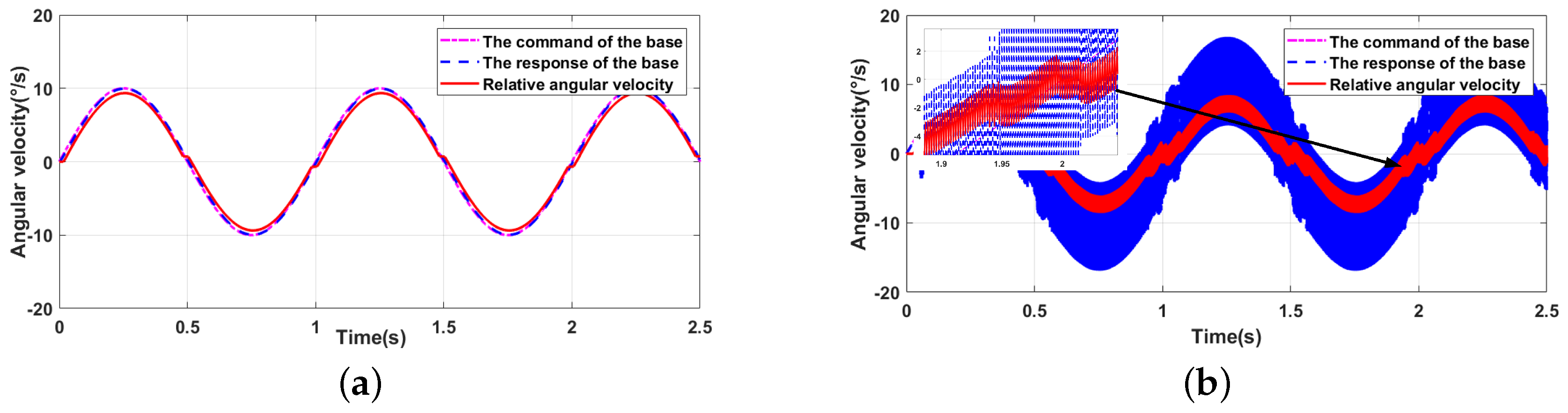
Based on the new dynamics model that uses the composite controller, under the same conditions in Section 2, the numerical analysis results are presented in Figure 4.

Compared with Figure 3, the vibration disappears, the tracking performance is better, and there is almost no phase lag for the low-frequency command. The composite controller can suppress the vibrations and achieve a high performance.

5. Experiments

To verify the effectiveness of the proposed method in suppressing the vibration and enhancing the control performance, an experimental system was built to compare the traditional and proposed methods.

5.1. Experimental Setup

The experimental set-up includes power, control board, base support, gyroscope, load, encoder, torque motor, and a computer. The system is illustrated in Figure 5.

The power supply of the whole system in the experiment consists of a 24 VDC switching power supply. The control board is developed based on DSP TMS320F28335. Development of the algorithm and data storage is achieved on the computer, and the sampling time is 0.001 s in the program. The torque motor is integrated with a harmonic drive and an incremental encoder. The key items of these devices are shown in

Table 2. Main devices used in the experiment.

Device	Model	Key Item
Gyroscope	STIM210 Multi-Axis Gyro Module	262 Hz (Bandwidth) $2^{-14\circ }$/s (Resolution)
Torque motor	RH-14D-3002-E100AL	5.9 Nm (Rated Torque)
Incremental Encoder	-	1000 (Pulses/revolution)
Harmonic drive	-	100 (Reduction Ratio)
Motor Driver	MAXON ESCON Module 50/5	5 A (Constant Current)

.

5.2. Parameter Selection and Identification

Based on the mechanical system finite element analysis results and the device parameters, the model parameters in the system are given in

Table 3. System parameters.

Symbol	Value
$J_m,J_b,J_l$	0.0014, 0.00075, 0.0008 [kg m${}^2$]
$B_m,B_b,B_l$	0.001, 0.001, 0.001 [kg m${}^2$/s]
$K_s$	10 [kg m${}^2$/s${}^2$]
$B_s$	0.01 [kg m${}^2$/s]
N	100
$K_a$	1 [kg m${}^2$/(s${}^2$V)]

.

First, to identify the friction model parameters, a low-frequency sine wave (0.005 Hz, 2 V) is used as the control voltage in the open-loop system to obtain the nonlinear disturbance for the model. The curve for the control voltage and the relative angular velocity are shown in Figure 6.

It is worth noting that when the control voltage approaches zero, the relative angular velocity exhibits a pronounced dead time phenomenon. $F_m\left(t\right)$ is similar to the theoretical friction model, and it is proven that the friction nonlinearity dominates the nonlinear disturbance. The friction feedforward method is designed to compensate its negative influence. If the NDOB is used in this system directly, there will be limitations to performance improvements. This is because the system may have a larger $\mathbf{d}\left(t\right)$ or $\dot{\mathbf{d}}\left(t\right)$ at some time, which is inconsistent with Assumption 1.

Friction torque $F_f\left(t\right)$ is fitted by the model (42). The relationship between the estimated disturbance torque and the relative angular velocity is shown in Figure 7.

In the experiments, the least squares method is used to fit the friction disturbance, and the friction nonlinear torque fitting parameters are obtained as shown in

Table 4. Nonlinear friction fitting parameters.

Symbol	Parameter	Value
$A_{c1},A_{c2}$	Coulomb friction magnitudes in the positive and negative direction	1.8, 2.0
$\gamma$	a large constant	100
$K_{v1},K_{v2}$	Viscous friction magnitudes in the positive and negative direction	0.005, 0.005

.

Second, to verify the model fitting accuracy and the effectiveness of the friction feedforward compensation method, the residual disturbance is estimated again. The control value and the residual disturbance curve are displayed in Figure 8.

Compared with Figure 7, the disturbance has been reduced from 3 V (peak to peak value) to less than 1 V. It shows the accuracy of the friction fitting value and the effectiveness of the friction feedforward method. From Figure 8, the residual disturbance and its first derivative are small constants like Assumption 1. The system performance will improve by increasing the NDOB gain, and the larger the gain, the stronger the ability to compensate for the disturbance. However, it will be considerably sensitive to sensor noise. Therefore, this parameter is selected in the trade-off between the disturbance suppression ability and noise sensitivity. The NDOB gain is 200 rad/s in the experiment.

Finally, the PI parameter can be adjusted by the sine or step response. The feedback controller parameters $u_c^{*}\left(t\right)$ are properly tuned to achieve optimum performance in practice, along with $K_p=1$ and $K_i=1$. The modified feedback controller is constructed in the form of Equation (29) with the following matrices.

$$\mathbf{A}=\left[\begin{array}{cc}0& 1\\ -30276& -139.2\end{array}\right]$$

(71)

$$\mathbf{B}={\left[\begin{array}{c}01\end{array}\right]}^T$$

(72)

$$\mathbf{C}=\left[\begin{array}{cc}0& -114.84\end{array}\right]$$

(73)

$$\mathbf{D}=1$$

(74)

The feedforward controller is easily obtained by the model parameters.

$$u_f\left(t\right)=\left[0.0010.0014\right]{\left[r_v\left(t\right)r_a\left(t\right)\right]}^T$$

(75)

5.3. Results and Discussion

To verify the vibration suppression effect and command tracking performance of the proposed method, a sine wave (1 Hz, 10${}^{\circ }$/s), which is a test command in engineering, is used as the angular velocity command. The experiments include five groups: A, B, C, D, and E. To simplify the description, the time-varying parameters $u_c\left(t\right),u_c^{*}\left(t\right),u_o\left(t\right),u_f\left(t\right)$ are represented by $u_c,u_c^{*},u_o,u_f$ in subsequent experiments. Group A uses the PI controller $u_c$ with a heavy base support. Group B uses the PI controller $u_c$ with a light base support and occurrence of vibrations. Group C uses the modified PI controller $u_c^{*}$ with a light base support in the form of Equation (28) to suppress the vibrations. Group D uses the proposed controller $u_c^{*}+u_o+u_f$ with a light base support in the form of Equation (27). Group E uses the controller $u_c+u_o+u_f$ with a light base support. Vibrations still occur, and in some instances, are even more pronounced. To be able to perform a one-on-one comparison for the experiments, the same PI parameters have been retained for the five groups. The sine command, the response curves, and the relative angular velocity error of the five groups are shown in Figure 9, Figure 10, Figure 11, Figure 12 and Figure 13. Furthermore, the root mean square errors (RMSEs) are shown in Figure 14.

In view of Figure 9, Figure 10, Figure 11, Figure 12, Figure 13 and Figure 14, the following conclusions can be drawn.

(a)

There is a significant nonlinear disturbance in the system, as demonstrated in Figure 9a, Figure 10a, and Figure 11a, especially when the angular velocity approaches zero. As a result, the system demonstrates a larger tracking error in Figure 9b, Figure 10b, and Figure 11b.

(b)

The base equivalent moment of inertia is lighter, and is more likely to cause system vibrations, as demonstrated in Figure 10a and Figure 13a.

(c)

Comparing Figure 10a and Figure 11a, the modified feedback controller effect is noticeable, and the vibrations are successfully suppressed.

(d)

In Figure 13a,b, without the modified feedback controller suppressing the vibrations, the composite controller will not suppress the vibrations, even when they are more pronounced.

(e)

Furthermore, the method proposed in this study shows great disturbance compensation and tracking performance improvements. The phase between the response and command in Figure 12a is ahead in comparison to Figure 11a. The relative angular velocity RMSE is reduced from 0.5165 ${}^{\circ }$/s to 0.3610 ${}^{\circ }$/s in Figure 14.

To find the vibration frequency more intuitively, we applied Fourier transforms to find the frequency components of a signal buried in the noise. Based on the experiments described above, the relative angular velocity is selected as the input signal. Thereafter, the Fourier transform of the signal is computed, the frequency domain is defined, and the single-sided amplitude spectrum is plotted. The amplitude is dimensionless. The results are presented in Figure 15.

From Figure 15, there is a peak of 26 Hz in Groups B and D, which has a negative effect on this system. If the modified controller (28) is used, the signal is redesigned. The vibration frequency is suppressed successfully similar to that in Groups A, C, and D.

In addition to the command tracking performance, another significant indicator for SISPs is the isolation used to measure the ability of disturbance isolation of the SISP. For a constant value disturbance or a periodic disturbance with constant amplitude, the isolation describes the system’s ability to restrain the disturbance under this frequency. If the disturbance is in a wide frequency range, the isolation can also be obtained by using the frequency characteristics. The smaller the isolation is, the stronger the system’s isolation ability and the better the LOS stability accuracy are. For this system, the inertial angular velocity after compensating is ${\dot{\theta }}_b\left(t\right)+{\dot{\theta }}_e\left(t\right)$, and the external disturbance inertial angular velocity is ${\dot{\theta }}_b\left(t\right)$, which is measured by the gyroscope. The amplitude-frequency curve from ${\dot{\theta }}_b\left(t\right)+{\dot{\theta }}_e\left(t\right)$ to ${\dot{\theta }}_b\left(t\right)$ is presented in Figure 16.

From Figure 16, the proposed method frequency isolation is lower than the PI control method in the SISP. The method proposed in this study has a positive external low-frequency disturbance effect. The isolation at a typical frequency of 1 Hz is taken as a quantitative comparison. The isolation of the PI feedback control is 3.37%, while the isolation of the proposed method is 1.54%.

6. Conclusions

Through a system model analysis, we were able to identify some limitations of the traditional model. In this study, a SISP multi-body dynamics model is established. Based on the new model, a composite controller is proposed to achieve high performance while suppressing the vibrations. The mathematical calculations and the experimental results verify the stability of the proposed controller. The experimental results also reveal that the proposed method can successfully suppress the vibration and improve the controller performance. Compared with the PI control methods, this newly developed method has a significant improvement in the tracking performance and the disturbance isolation. The RMSE of the relative angular velocity is reduced from 0.5165 ${}^{\circ }$/s to 0.3610 ${}^{\circ }$/s, and the isolation is reduced from 3.37% to 1.54%. The significant contribution of the proposed method is that the SISP model was established with a light base support and a modified feedback controller was designed according to the vibration characteristics. Combining the disturbance controller and the feedforward controller, high-precision control performance was achieved, and inertial stability of the LOS was realized. These performance improvements are significant in the fields of science and engineering.

In future work, an advanced control method, such as SMC, adaptive control, or the $H_{\infty }$ control, will be used to further enhance the control performance while suppressing the vibrations.

References

1. Hilkert, L. Inertially Stabilized Platform Technology Concepts and Principles. IEEE Control Syst. Mag. 2008, 28, 26–46. [Google Scholar]
2. Dong, F.; Lei, X.; Chou, W. A Dynamic Model and Control Method for a Two–Axis Inertially Stabilized Platform. IEEE Trans. Ind. Electron. 2017, 64, 432–439. [Google Scholar] [CrossRef]
3. Li, S.; Zhong, M. High–Precision Disturbance Compensation for a Three–Axis Gyro–stabilized Camera Mount. IEEE/ASME Trans. Mechatron. 2015, 20, 3135–3147. [Google Scholar] [CrossRef]
4. Cui, P.; Zhang, D.; Yang, S.; Li, H. Friction Compensation Based on Time-Delay Control and Internal Model Control for a Gimbal System in Magnetically Suspended CMG. IEEE Trans. Ind. Electron. 2017, 64, 3798–3807. [Google Scholar] [CrossRef]
5. Özkan, B.; Uçar, A. Comparison of the Strapdown and Gimbaled Seekers Utilized in Aerial Applications. Infrared Technol. Appl. 2012, 8353, 83530. [Google Scholar]
6. Zhang, L.; Li, B.; Wang, Q.; Yi, J. Research on Electronic Image Stabilization Based on Carrier Decoupling. In Proceedings of the 3rd International Congress on Image and Signal Processing, Yantai, China, 16–18 October 2010; pp. 801–805. [Google Scholar]
7. Tian, D.; Shen, H.; Dai, M. Improving the Rapidity of Nonlinear Tracking Differentiator via Feedforward. IEEE Trans. Ind. Electron. 2014, 61, 3736–3743. [Google Scholar] [CrossRef]
8. Roozing, W.; Malzahn, J.; Caldwell, D.; Tsagarakis, N. Comparison of Open–Loop and Closed–Loop Disturbance Observers for Series Elastic Actuators. In Proceedings of the IEEE/RSJ International Conference on Intelligent Robots and Systems, Daejeon, Korea, 9–14 October 2016; pp. 3842–3847. [Google Scholar]
9. He, W.; Yan, Z.; Sun, C.; Chen, Y. Adaptive Neural Network Control of a Flapping Wing Micro Aerial Vehicle With Disturbance Observer. IEEE Trans. Cybern. 2017, 47, 3452–3465. [Google Scholar] [CrossRef]
10. Ahi, B.; Nobakhti, A. Hardware Implementation of an ADRC Controller on a Gimbal Mechanism. IEEE Trans. Control Syst. Technol. 2018, 26, 2268–2275. [Google Scholar] [CrossRef]
11. Huang, Y.; Xue, W. Active disturbance rejection control: Methodology and theoretical analysis. ISA Trans. 2018, 53, 963–976. [Google Scholar] [CrossRef]
12. Wen, G.; Ge, S.; Tu, F.; Choo, Y. Artificial Potential–Based Adaptive H Synchronized Tracking Control for Accommodation Vessel. IEEE Trans. Ind. Electron. 2017, 64, 5640–5647. [Google Scholar] [CrossRef]
13. Li, Z.; Su, C.; Wang, L.; Chen, Z.; Chai, T. Nonlinear Disturbance Observer-Based Control Design for a Robotic Exoskeleton Incorporating Fuzzy Approximation. IEEE Trans. Ind. Electron. 2015, 62, 5763–5775. [Google Scholar] [CrossRef]
14. Chen, W.; Yang, J.; Guo, L.; LI, S. Disturbance–Observer–Based Control and Related Methods—An Overview. IEEE Trans. Ind. Electron. 2016, 63, 1083–1095. [Google Scholar] [CrossRef] [Green Version]
15. Sariyildiz, E.; Oboe, R.; Ohnishi, K. Disturbance Observer–Based Robust Control and Its Applications: 35th Anniversary Overview. IEEE Trans. Ind. Electron. 2020, 67, 2042–2053. [Google Scholar] [CrossRef] [Green Version]
16. Wei, X.; Guo, L. Composite disturbance–observer–based control and H–infinity control for complex continuous models. Int. J. Robust Nonlinear Control 2010, 20, 106–118. [Google Scholar] [CrossRef]
17. Guo, L.; Chen, W. Disturbance Attenuation and Rejection for Systems with Nonlinearity via DOBC Approach. Int. J. Robust Nonlinear Control 2005, 15, 109–125. [Google Scholar] [CrossRef]
18. Yang, J.; Li, S.; Yu, X. Sliding–Mode Control for Systems With Mismatched Uncertainties via a Disturbance Observer. IEEE Trans. Ind. Electron. 2013, 60, 160–169. [Google Scholar] [CrossRef]
19. Guo, L.; Wen, X. Hierarchical anti–disturbance adaptive control for nonlinear systems with composite disturbances and applications to missile systems. Trans. Inst. Meas. Control 2011, 8, 942–956. [Google Scholar] [CrossRef]
20. Mao, J.; Li, S.; Li, Q.; Yang, J. Design and implementation of continuous finite–time sliding mode control for 2–DOF inertially stabilized platform subject to multiple disturbances. ISA Trans. 2019, 84, 214–224. [Google Scholar] [CrossRef] [PubMed]
21. Singh, S.; Marathe, R.; Kumar, A.; Kumar, R. Sliding Mode Control based Line–of–Sight (LOS) Stabilization of Electro-optical Sighting System. In Proceedings of the 1st IEEE International Conference on Power Electronics, Intelligent Control and Energy Systems, Delhi, India, 4–6 July 2016; pp. 1–6. [Google Scholar]
22. Safa, A.; Abdolmalaki, R. Robust Output Feedback Tracking Control for Inertially Stabilized Platforms with Matched and Unmatched Uncertainties. IEEE Trans. Control Syst. Technol. 2019, 27, 118–131. [Google Scholar] [CrossRef]
23. Deng, K.; Cong, S.; Kong, D.; Shen, H. Discrete–Time Direct Model Reference Adaptive Control Application in a High-Precision Inertially Stabilized Platform. IEEE Trans. Ind. Electron. 2019, 66, 358–367. [Google Scholar] [CrossRef]
24. Wang, F.; Wang, R.; Liu, E.; Zhang, W. Stabilization Control Mothed for Two–Axis Inertially Stabilized Platform Based on Active Disturbance Rejection Control With Noise Reduction Disturbance Observer. IEEE Access 2019, 7, 99521–99529. [Google Scholar] [CrossRef]
25. Na, J.; Chen, Q.; Ren, X.; Guo, Y. Adaptive Prescribed Performance Motion Control of Servo Mechanisms with Friction Compensation. IEEE Trans. Ind. Electron. 2014, 61, 486–494. [Google Scholar] [CrossRef]
26. Yao, J.; Deng, W.; Jiao, Z. Adaptive Control of Hydraulic Actuators With LuGre Model–Based Friction Compensation. IEEE Trans. Ind. Electron. 2015, 62, 6469–6477. [Google Scholar] [CrossRef]
27. Tsai, M.; Chiu, I.; Cheng, M. Design and implementation of command and friction feedforward control for CNC motion controllers. IEE Proc. Control Theor. Appl. 2004, 151, 13–20. [Google Scholar] [CrossRef]
28. He, W.; Li, Z.; Chen, P. A survey of human–centered intelligent robots–Issues and challenges. IEEE/CAA J. Autom. Sin. 2017, 4, 602–609. [Google Scholar] [CrossRef]
29. He, W.; Dong, Y. Adaptive Fuzzy Neural Network Control for a Constrained Robot Using Impedance Learning. IEEE Trans. Neural Netw. Learn. Syst. 2018, 29, 1174–1186. [Google Scholar] [CrossRef]
30. Wang, Y.; Bian, N.; Li, J.; Yuan, J.; Chen, H. A triple–step non–linear control for path following of autonomous vehicles with uncertain kinematics and dynamics. IET Control Theory A 2017, 11, 3381–3387. [Google Scholar] [CrossRef]
31. Kennedy, C.; Desai, J. Modeling and Control of the Mitsubishi PA–10 Robot Arm Harmonic Drive System. IEEE Trans. Mechatron. 2005, 10, 263–274. [Google Scholar] [CrossRef]
32. Hadas, Z.; Garami, B. Mechatronic Model of Harmonic Drive System. In Proceedings of the 17th International Conference on Mechatronics–Mechatronika, Prague, Czech Republic, 7–9 December 2016; pp. 1–6. [Google Scholar]
33. Liu, Y.; Sun, L.; Meng, Q. Acceleration Feedback Control of a Harmonic Drive Parallel Robot. In Proceedings of the IEEE Conference on Robotics, Automation and Mechatronics, Singapore, 1–3 December 2004; pp. 390–395. [Google Scholar]
34. Lu, Y.; Hwang, C. Tracking Control of a Harmonic Drive Actuator with Sliding–Mode Disturbance Observers. In Proceedings of the IEEE/ASME International Conference on Advanced Intelligent Mechatronic, Singapore, 14–17 July 2009; pp. 1798–1803. [Google Scholar]
35. Zhu, W. Precision Control of Robots with Harmonic Drives. In Proceedings of the IEEE International Conference on Robotics and Automation, Roma, Italy, 10–14 April 2007; pp. 3831–3836. [Google Scholar]
36. Roozing, W.; Malzahn, J.; Kashiri, N.; Caldwell, D.; Tsagarakis, N. On the Stiffness Selection for Torque–Controlled Series–Elastic Actuators. IEEE Robot. Autom. Lett. 2017, 2, 2255–2262. [Google Scholar] [CrossRef]
37. Yamamoto, M.; Iwasaki, M.; Kainum, M.; Okitsu, Y. Compensation for Synchronous Component of Angular Transmission Errors in Harmonic Drive Gearings. In Proceedings of the 11th IEEE International Workshop on Advanced Motion Control, Nagaoka, Japan, 21–24 March 2010; pp. 361–365. [Google Scholar]
38. de Wit, C.C.; Olsson, H.; Astrom, K.J.; Lischinsky, P. A new model for control of systems with friction. IEEE Trans. Autom. Control 1995, 40, 419–425. [Google Scholar] [CrossRef] [Green Version]
39. Hassan, K. Nonlinear Systems, 3rd ed.; Prentice Hall: Upper Saddle River, NJ, USA, 2002. [Google Scholar]
40. Sariyildiz, E.; Sekiguchi, H.; Nozaki, T.; Ugurlu, B.; Ohnish, K. A Stability Analysis for the Acceleration–Based Robust Position Control of Robot Manipulators via Disturbance Observer. IEEE/ASME Trans. Mechatron. 2018, 23, 2369–2378. [Google Scholar] [CrossRef]
Figure 1. Schematic diagram of a typical three-axis strapdown inertially stabilized platforms (SISP) for the moving base carrier.
Applsci 10 07175 g001
Figure 2. Control system diagram. (a) Motor; (b) Harmonic drive; (c) Load.
Applsci 10 07175 g002
Figure 3. Numerical analysis results. (a) Light load with J l = 0.001 ; (b) Heavy load with J l = 0.01 .
Applsci 10 07175 g003
Figure 4. Results of the numerical analysis used in the composite controller.
Applsci 10 07175 g004
Figure 5. Experimental set-up.
Applsci 10 07175 g005
Figure 6. Control voltage and response in the open-loop system.
Applsci 10 07175 g006
Figure 7. Disturbance torque fitting and the estimation values.
Applsci 10 07175 g007
Figure 8. Residual disturbance curve.
Applsci 10 07175 g008
Figure 9. Group A: PI controller u c with a heavy base support. (a) Sine command and relative angular velocity; (b) Relative angular velocity error.
Applsci 10 07175 g009
Figure 10. Group B: PI controller u c with a light base support. (a) Sine command and relative angular velocity; (b) Relative angular velocity error.
Applsci 10 07175 g010
Figure 11. Group C: Modified PI controller u c * with a light base support. (a) Sine command and relative angular velocity; (b) Relative angular velocity error.
Applsci 10 07175 g011
Figure 12. Group D: Proposed controller u c * + u o + u f with a light base support. (a) Sine command and relative angular velocity; (b) Relative angular velocity error.
Applsci 10 07175 g012
Figure 13. Group E: Controller u c + u o + u f with a light base support. (a) Sine command and relative angular velocity; (b) Relative angular velocity error.
Applsci 10 07175 g013
Figure 14. Angular velocity root mean square error (RMSE).
Applsci 10 07175 g014
Figure 15. Single-sided dimensionless amplitude spectrum of the relative angular velocity. (a) Group A; (b) Group B; (c) Group C; (d) Group D; (e) Group E.
Applsci 10 07175 g015
Figure 16. Frequency isolation curve.
Applsci 10 07175 g016