Numerical Modeling of Surface Water and Groundwater Interactions Induced by Complex Fluvial Landforms and Human Activities in the Pingtung Plain Groundwater Basin, Taiwan

Abstract

The landforms and human activities play important roles in quantifying surface water and groundwater interactions (SGIs) for water resources management. The study uses the groundwater and surface water flow (GSFLOW) model to quantify the dynamics of SGIs in the Pingtung Plain groundwater basin (PPGB) in southern Taiwan. Specifically, the study uses a physical-based numerical model to quantify the spatial and seasonal variations of water cycles influenced by complex fluvial landform conditions and human activities. Results of the model calibrations show good agreement with the data obtained from the available groundwater monitoring network and the selected stream stations. The basin-scale water budgets show highly nonuniform precipitation in the study area, and over 80% annual precipitation is from wet seasons in the PPGB. With high permeable surficial deposits in the PPGB, the year-averaged surface runoff and infiltration are approximately 57% and 40% of the total precipitation. The fluvial landforms with the high slope in the PPGB lead to 70% of annual surface runoff that becomes the streamflow, and the interflow dominates water interactions near streambeds. Results show that the interflow rate in the wet seasons is 200% more than that in the dry seasons. The net groundwater discharge to the streams is relatively small as compared to the interflow. Only 10% of the river flow is from the net groundwater discharge. In the PPGB, The pumping-induced variations of groundwater levels are insignificant as compared with the factor of the natural landforms. Because of the relatively small area of the proposed artificial lake, the contribution of the artificial lake on the local water budgets is insignificant, indicating the low impact of the artificial recharge lake on the surface water environment.

1. Introduction

Hydrologic models have been developed and implemented for simulating surface water and groundwater dynamics and assessing the interactions between them. The quantification of surface water and groundwater interactions (SGIs) typically considers the influences of rainfall, evapotranspiration, or groundwater pumping in a specific groundwater basin [1]. With the advantages of computational technologies, the integrated hydrologic models (IHMs) have made the coupled solutions possible to analyze complex water resource problems relevant to the interactions of surface water and groundwater systems. The processes included in the IHMs can be the overland flow, surface runoff, infiltration, evapotranspiration, soil zone flow, or groundwater interactions and others [2]. In IHMs, the coupled surface and subsurface flow equations are solved either simultaneously or iteratively [3]. These types of models are physical-based models because the physical mechanisms are considered based on the concepts of mass, momentum, or energy conservations. The parameters in the equations can represent physical properties in either the surface water or the groundwater systems. Depending on the complexity of the developed models, the coupled equations in IHMs can be one- or multi-dimensional problems. The implementations of IHMs require comprehensive knowledge of the detailed theory of the IHMs so that the practical problems can be accurately solved.

Intensive studies have developed numerous IHMs to assess interactions between surface water and groundwater systems. These widely used models include the SWATMOD model [4], parallel groundwater flow (PARFLOW) model [5], MODHMS model [6], 3D fully coupled groundwater-surface model (an acronym for catchment hydrology model, CATHY) [7], HydroGeoSphere model [8], WetSpass-MODFLOW [9], J2000-MODFLOW model [10], GSFLOW model [11], and MIKE SHE [12]. The SWATMOD model couples the soil water assessment tool (SWAT) model [13] with the three-dimensional groundwater simulation (MODFLOW) model [14]. The MODHMS model considers two-dimensional diffusion surface flow and has been integrated into the MODFLOW model. The main focus of the MODHMS is the dynamics of the surface water flow that provide detailed sources for the MODFLOW model. MIKE SHE is an integrated water resources model that enables the simulations of coupled surface and subsurface water dynamics. The particle-based random walk approach was used in the model to simulate the processes that affect surface water quality. The HydroGeoSphere model allows for simulating stream and surface drainage networks that physically connect rivers to the groundwater systems. The special feature of the model is that the model avoids the problems related to the riverbed-conductance concept, which is a challenging task for most practical implementations. The CATHY model is a process-based model that focuses on quantifying the spatio-temporal variability of soil moisture, groundwater flow and surface runoff. The WetSpass-MODFLOW model is used to evaluate the feasibility of water replenishment through natural reservoirs. The model integrated a spatially-distributed water balance model (WetSpass-M), and a groundwater flow model (MODFLOW-NWT). J2000 is a package that is developed based on the software environment of the geographical information system (GIS). The model is a hydrological model that provides the water balance near the land surface for the MODFLOW focusing on the large catchment areas.

The GSFLOW model has integrated the Precipitation Runoff Modeling System (PRMS) [15] with MODFLOW to account for interactions between surface water and groundwater. The GSFLOW model is also a physical-based model developed by the U.S. Geological Survey (USGS). The advantages of the GSFLOW model are the efficiency of PRMS modules and the well-developed MODFLOW-2005 packages that can provide detailed dynamics of groundwater flow. The model uses a flexible and adaptive modular design framework and allows simulations to be performed by only PRMS or MODFLOW-2005, or both. In the GSFLOW model, the coupling process employs iterative techniques to solve interdependent governing equations for surface water and groundwater flow. The calculations of detailed water balances in time and space are available in the models. The model also allows flexible spatial discretization of the hydrologic response units (HRUs) used for PRMS and the finite-difference grid used for MODFLOW-2005 [11]. Critical connections in the GSFLOW model refer to the unsaturated flow as well as stream interaction modules in MODFLOW.

The important processes of SGIs are influenced by land-use change, climate variability, and groundwater exploitations. The interactions of surface water and groundwater play essential roles in hydro-environmental and eco-hydrological systems for a groundwater basin. The effects of agricultural activities such as surface water allocations, groundwater pumping, and irrigation on interactions of surface water and groundwater are very complex, which can significantly change the behavior of surface water and groundwater flow interactions [16]. Understanding the complicated behavior of SGI is very important for regional water resources management. Existing models have been intensively developed for addressing different water resources issues such as irrigation management, SGIs, land-use, climate change and water quality. In many previous studies, the GSFLOW model was applied to simulate the interactions between surface water and groundwater flows for interested watersheds [17,18]. In view of the complex amounts of input data established in the GSFLOW model, the development of a simulation model for a case study covering a large area with multiple watersheds is a great challenge.

The Pingtung Plain groundwater basin (PPGB) is located in southwest Taiwan and bounded by the Taiwan Strait to the south. The PPGB has a relatively large area, a dense river system, and the land surface elevation varies significantly. Due to the combination of natural processes (i.e., tectonic deformation, surficial deposition, and precipitation) and human activities (i.e., land-use and hydraulic infrastructures) applied to the PPGB, the landforms have evolved differently over time in the upstream and downstream areas in the PPGB. The highly non-uniform precipitation is obtained in wet and dry seasons, leading to strong fluctuations of river and groundwater levels. The variation of rainfall is evident in the upstream fan area of the PPGB. Understanding the dynamics of the SGI in the PPGB is the critical element to propose efficient strategies for water resource management. The effects of complex landforms and human activities have to be clarified before the implementation of the IHMs in the PPGB. The present study utilizes the GSFLOW numerical model to assess the SGIs in PPGB. The study aims to characterize the behaviors and dynamics of SGIs and to quantify the influence of interactions induced by the natural and anthropogenic effects. Specifically, the PPGB was divided into the upstream and downstream areas based on the flow patterns of the river system. The water balance for each component in the water cycle was systematically evaluated and quantified according to the detailed interaction dynamics in the PPGB. The calibration and validation of the model are based on three-year observations from January 2015 to December 2017. The evaluation of the developed model relies on different statistical parameters such as the coefficient of determination (R²), coefficient of correlation (RE), Nash-Sutcliffe efficiency coefficient (NSE), normalized root-mean-square deviation (NRMSE), and percent bias (Pbias). A scenario of an artificial recharge reservoir was considered to assess the local impact of increased recharge on water balance variations in the simulation area.

2. Materials and Methods

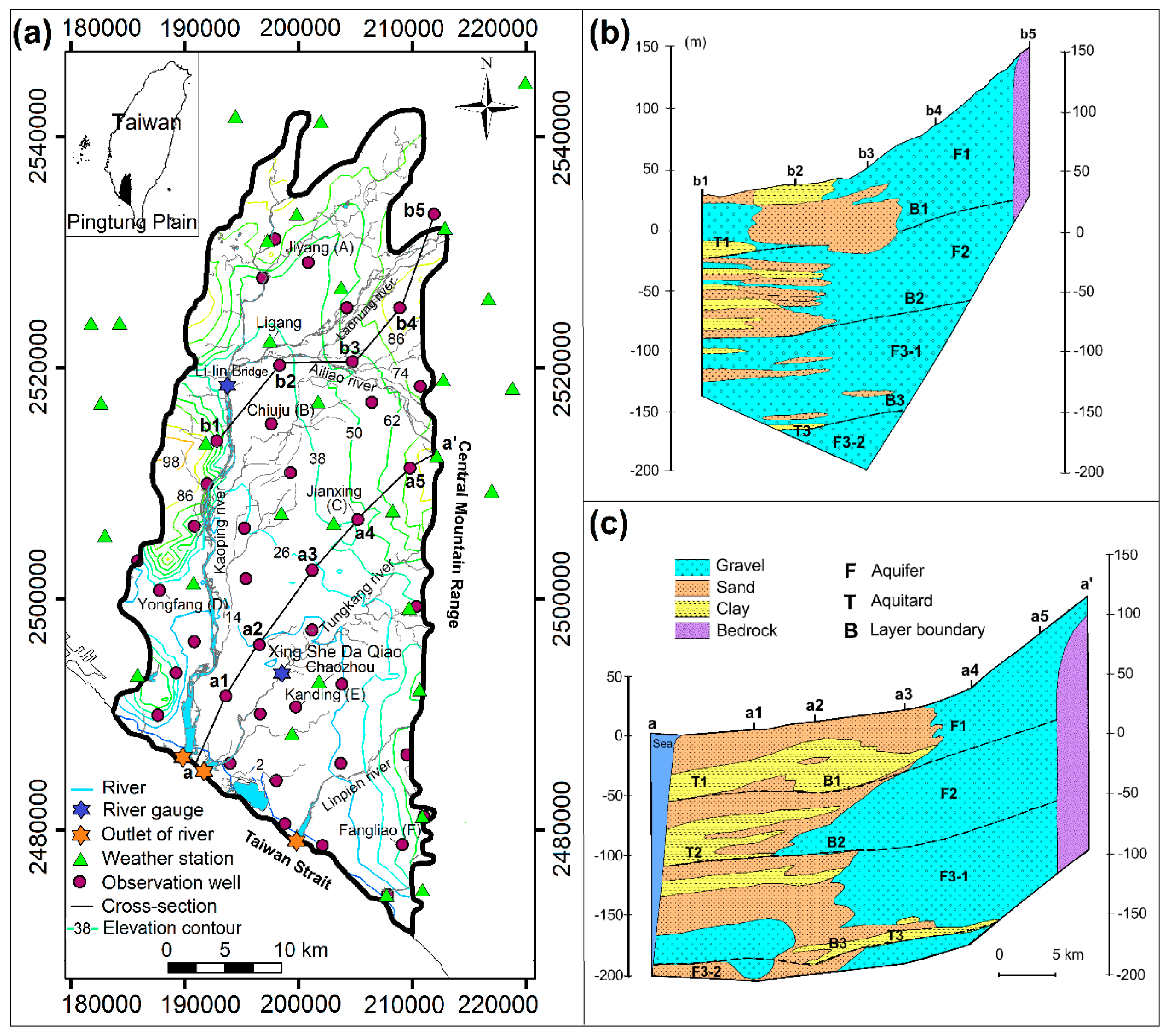
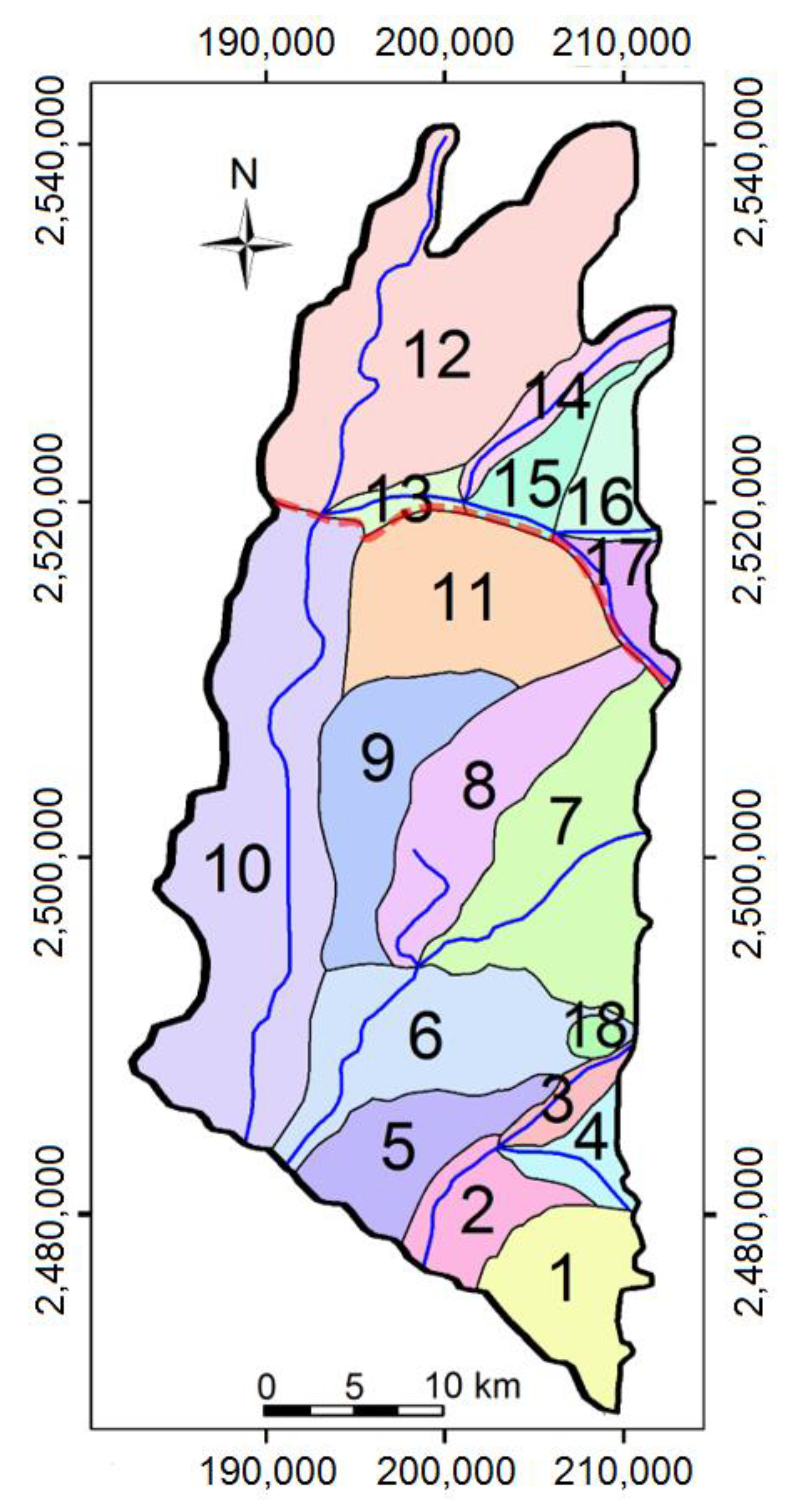
2.1. Study Area

The PPGB is located in southern Taiwan and bounded by the low hills of sediments to the north, the foothills to the west, the Central Mountain Range to the east, and the Taiwan Strait to the south (see Figure 1). The oblique collision between the Philippine Sea Plate and the continental margin of the Eurasian Plate forms Taiwan Island and leads to a series of north-south mountain ranges and active fold-and-thrust belts [19]. The area covers approximately 1300 km², land surface elevation varies from the north about 100 m to the south approximately 0 m (see the contours shown in Figure 1a). The climate in PPGB is subtropical and rainfall is alternately affected by typhoons and monsoons in dry and wet seasons. Typhoons and thunderstorms regularly occur in wet seasons and are the leading cause of heavy rainfall. According to climate statistics for the period between 2010 and 2018, the annual precipitation in the PPGB varied significantly from 1431 to 3597 mm, and the average precipitation was 2331 mm. Figure 1 also shows the precipitation stations and the monitoring wells network developed in the groundwater basin. The long-term records of regional precipitation have demonstrated that the rainy season in the groundwater basin is from May to October and the dry season is from November to April in the next year. Specifically, the rainfall in the dry season is mainly affected by monsoons and total precipitation is about 10 percent of that during the rainy season. The Kaoping River flows from north to south and is the largest river along the western foothills with an average slope of 1:43. The coupled natural processes (i.e., tectonic deformation and surficial deposition) and human activities (i.e., land-use and hydraulic infrastructures) altered the landscape in the upstream and downstream fan areas in the PPGB. In the study, the upstream fan is defined as the upstream area of the confluence point (i.e., the Li-lin Bridge) of the Kaoping River, where Ailiao and Laonung Rivers mainly flow in the east-west direction. In the downstream fan area, the flow directions of the Kaoping, Tungkang, and Linpien Rivers are generally in a north-south direction to the Taiwan Strait. The downstream fan area is also the region that had faced severe problems in groundwater over-pumping and groundwater contamination [20].

The aquifer of the PPGB mainly consists of unconsolidated Quaternary deposits. The mountainous regions surrounding the PPGB are composed of Tertiary rocks [21]. The rocks of the Suao Group Formation are of Eocene-Oligocene age, located in the eastern part of the plain. The Chaozhou fault, stretching from north to south, separates the Suao Group Formation and the PPGB. Hundreds of meters of recent alluvium formed the groundwater basin. However, the maximum thickness of sediments of the recent alluvium is not determined because drilling logs have not shown the bedrock floor during the installation of wells. This recent alluvium includes three material types, including coarse gravel, alternating gravel and sand, and fine material zones. These unconsolidated sediments are also the primary materials distributed on the surface of the PPGB. The hydrogeological surveys were conducted since 1995. A groundwater monitoring network was also developed based on the characterization of hydrogeological surveys. In the PPGB, the monitoring network was designed to monitor groundwater levels in different aquifer layers. Fifty-one hydrogeological investigation stations and 126 monitoring wells are available in the groundwater basin [22]. Based on the hydrogeological surveys, the sediment deposits in the downstream fan area can be further divided into four aquifer layers, separated by low permeable marine sequences (Figure 1). There are no marine sequences obtained in the upstream fan area of the PPGB [22]. The processes to develop the groundwater monitoring network also included pumping tests for the wells. However, very little information is available for the aquitards because the monitoring network was designed for monitoring the regional groundwater supply.

In the study, the development of the groundwater model followed the conceptual layers defined by Taiwan CGS [22], and the groundwater flow model was calibrated based on the data obtained from the monitoring network. With the relatively high slope of the land surface in the upstream fan area and highly non-uniform precipitation in wet and dry seasons, the surface water and groundwater monitoring networks show strong fluctuations of river and groundwater levels. In the PPGB, the groundwater recharge varies significantly between the wet and dry seasons and is influenced considerably by land cover and slope. In the study, we considered the first layer of the PPGB as the target aquifer to assess the interactions of groundwater and surface water. There are 39 observation wells considered for the model calibration. The interpolated climate observations for the surface water flow model (i.e., PRMS) were obtained from 21 rain stations near the PPGB (see Figure 1). We collected the weather data of maximal and minimal temperature and precipitation from two weather stations (i.e., the Ligang and Chaozhou stations). The locations of the stations are near two river gauges (i.e., the Li-lin Bridge and Xing She Da Qiao stations). The rainfall data obtained from the stations show that the total rainfall for the years 2015, 2016, and 2017 are 1912, 3796, and 1864 mm, respectively. Significant variations of rainfall were obtained in the study area. The conditions with high variations of precipitation in the study area are the main challenge for model calibration and verification. However, the significant variations of the extreme conditions are the basis to illustrate the important behaviors and dynamics of SGIs in the study area.

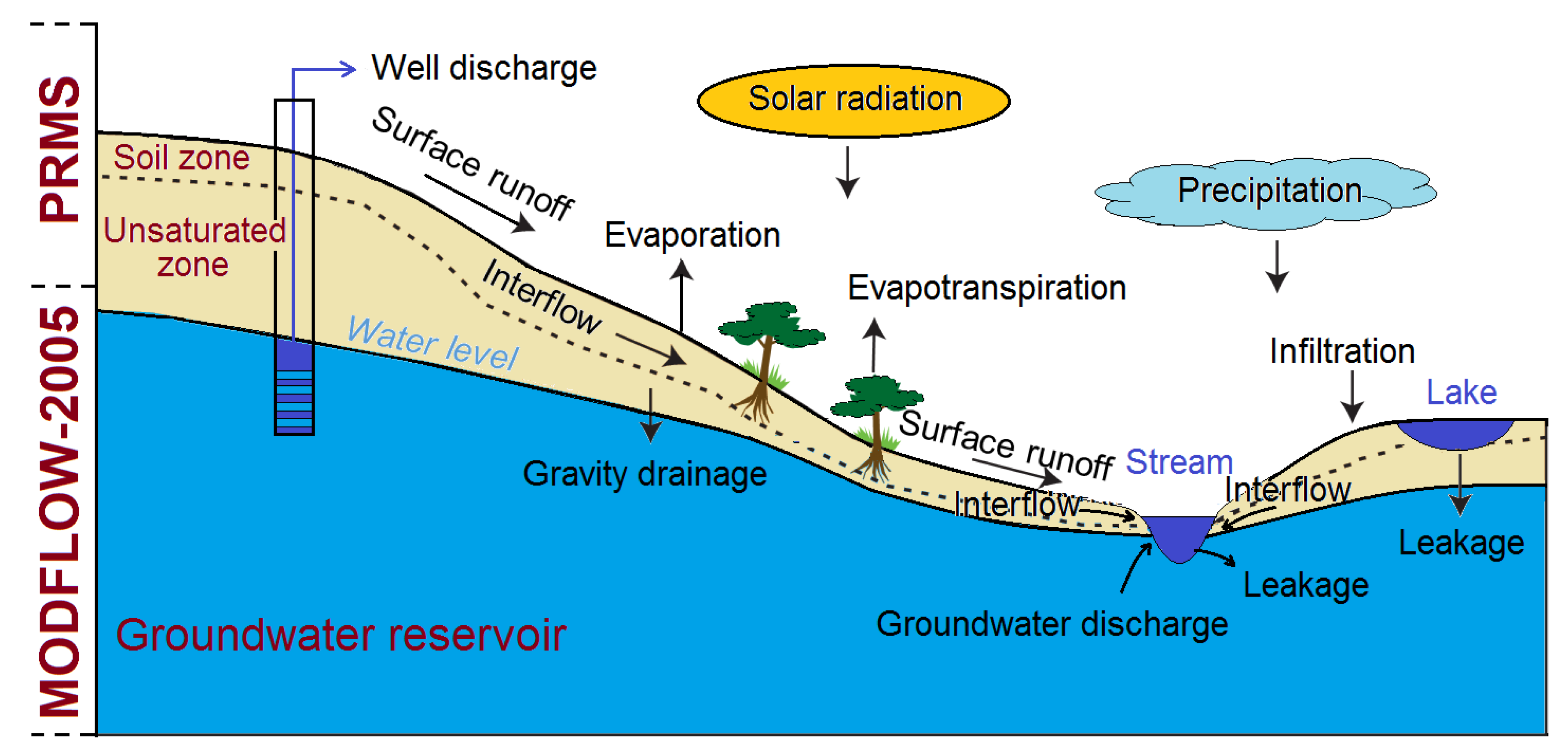
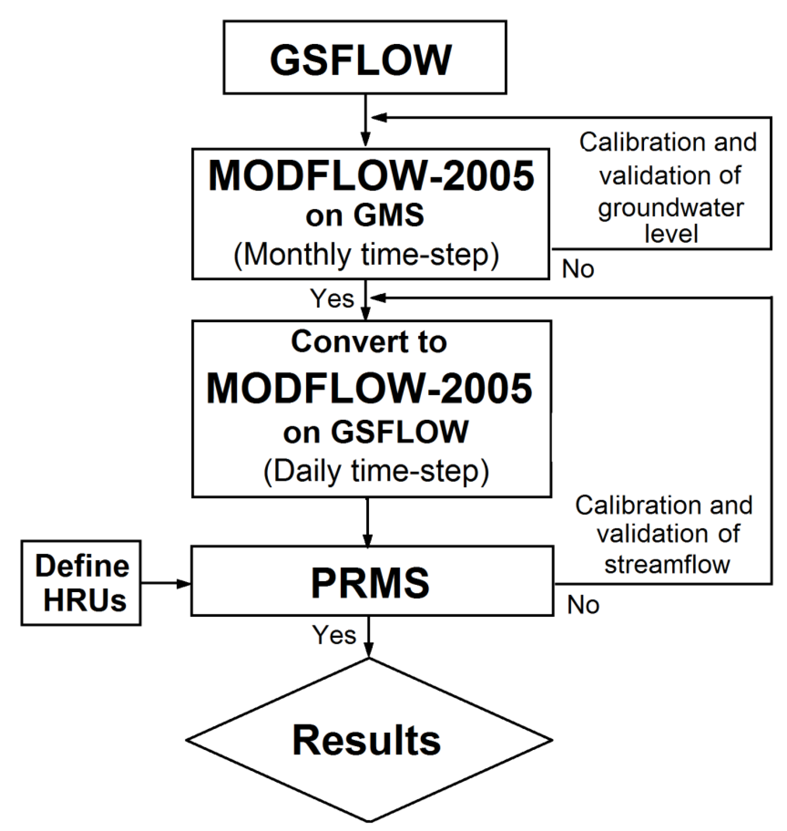
2.2. Modeling Framework

The GSFLOW model coupled the Precipitation Runoff Modeling System (PRMS) with the 2005 version of the Modular Groundwater Flow Model (i.e., MODFLOW-2005). The GSFLOW model can run either PRMS-only or MODFLOW-2005-only or both. There are three conceptual regions involved in the GSFLOW model (Figure 2). The first region is between the plant canopy on the top and the soil zone on the bottom. The second region consists of streams and lakes. The third region is beneath the soil zone. In the GSFLOW model, the responses of the hydrologic processes in the first region are simulated by the PRMS model. However, the processes in two other regions are simulated with the MODFLOW-2005 model. Because the GSFLOW model integrates many simulation modules, the formats, contents, and module communications must be defined in the input files for both PRMS and MODFLOW models. All the formats of input files in the GSFLOW model had been organized based on modular modeling system files [23] and followed the standard MODFLOW-2005 input requirements [14].

The PRMS model can be used to simulate and assess the effects of the various combinations of climate, and land-use on the watershed response based on changes in water balance relations, streamflow regimes, soil-water relations, and groundwater recharges. The PRMS model uses a series of reservoirs to simulate the hydrologic processes of the watershed. A watershed is an area or ridge of land that separates water that flows to different rivers, basins, or sea. The streamflow and detention reservoir segments to the drainage network are simulated by surface runoff, interflow, and groundwater discharge. In the PRMS model, the calculations of evaporation, transpiration, surface runoff, and infiltration require different types of climate data. These data include precipitation, air temperature, and solar radiation [15]. When the precipitation reaches the land surface, the water may be stored in the sealed zone, infiltrated into the soil zone, evaporated, or become surface runoff. In the PRMS model, the subsurface is represented by three conceptual reservoirs, namely the soil zone, unsaturated zone, and groundwater reservoir. The soil and unsaturated zones account for the different fractions of volumetric water flowing downslope, which may be further removed by plants or combined with groundwater. The water in the soil zones may become surface runoff, interflow, and recharge. It can still be lost because of the evaporation and transpiration based on plant type, solar radiation, and air temperature. The water stored in the unsaturated zones can be available for the gravity drainage to the groundwater reservoirs or for the interflow that flows to the streams or lakes. The water stored in the groundwater reservoirs can become available for the groundwater discharge to streams or be lost to subsurface sinkholes.

In the study, the watersheds in the GSFLOW model were discretized into many specified hydrologic response units (HRUs). The discretization and determination of the HRUs are based on site-specific hydrologic and physical characteristics, including drainage boundary, land-surface altitude, land-surface slope, land-surface aspect, plant type, plant cover, land-use, precipitation distribution, temperature distribution, solar radiation distribution, soil morphology, geology, or flow direction [11]. Each HRU is assumed to be homogeneous to represent the hydrologic and physical characteristics. The flow paths and fluxes in each HRU and the adjacent HRUs are computed based on the concept of mass conservation and user-defined input data and model parameters in the GSFLOW model. Note that the simulations of watershed responses are discretized into a daily time-step model to handle the daily observations of precipitation, air temperature, and solar radiation.

In the study, the groundwater flow processes, such as areal recharge, leakage from streamflow to aquifers, groundwater discharge to streams, and groundwater pumping, were simulated by using the MODFLOW-2005 model. The features of the MODFLOW-2005 are to model the three-dimensional steady or transient flow of groundwater through porous media. The unsaturated zone flow (UZF) package [24] used in MODFLOW-2005 was available for simulating the flow through the unsaturated zone. The package, associated with the PRMS module, can adequately account for the complex water interactions between the land surface and unsaturated zones above the groundwater levels. In the MODFLOW-2005, the movement of the groundwater flow with the constant density can be described by the following formula [14]:

$$S\frac{\partial h}{\partial t}=\frac{\partial }{\partial x}(K_x\frac{\partial h}{\partial x})+\frac{\partial }{\partial y}(K_y\frac{\partial h}{\partial y})+\frac{\partial }{\partial z}(K_z\frac{\partial h}{\partial z})+W$$

(1)

where notations $K_x$, $K_y$, $K_z$ [L/T] are the hydraulic conductivity in the x-, y-, and z-directions, $h=h(x,y,z,t)$ [L] is the hydraulic head. Notation $W=W(x,y,z,t)$ [1/T] is a volumetric flux per unit volume, representing sources and sinks of an aquifer system. The parameter $S$ is the storage coefficient of the aquifer, and $t$ [T] is time. In MODFLOW-2005, based on solving Equation (1) the boundary conditions can be the constant hydraulic head, the specified hydraulic head, or the default no-flow boundary conditions surrounding the simulation domain.

The unsaturated zone flow package considers the effects of flow, evapotranspiration, and storage in the unsaturated zone. The package plays an important role in coupling MODFLOW-2005 with many precipitation-runoff models [24]. In the UZF package, the equation used to model unsaturated flow is the one-dimensional Richards’ equation, which has the following formula:

$$\frac{\partial \theta }{\partial t}+\frac{\partial K(\theta )}{\partial z}+i=0$$

(2)

where $\theta$ [L³/L³] is the volumetric water content and $z$ [L] is the altitude in the vertical direction. The notation $K(\theta )$ [L/T] is the unsaturated hydraulic conductivity, determined by the unsaturated water content $\theta$. Notation $i$ [L²/T] is the evapotranspiration rate per unit depth beneath the soil zone. In the MODFLOW model, the analytical solution to Equation (2) was developed by using the method of characteristics (MOC) to solve for hyperbolic types of partial differential equations in which the solution can be integrated along the characteristic line from a given initial state. Previous investigations had extended the solution to account for the evapotranspiration loss for site-specific conditions [24].

3. Conceptual Models and Numerical Considerations

The study aims to characterize the SGI behavior in the PPGB and quantify the influence of such interactions induced by the natural and anthropogenic activities. There were selected components in the water balance to assess the variations of interaction dynamics in dry and wet seasons. The study conducted model calibration and validation by using the data from January 2015 to December 2017. More specifically, the data in 2015 were for the model calibration, while the data in 2016 and 2017 were for the model validation.

Figure 3 shows the workflow of the study for the GSFLOW simulations. In the study, the preparation of computational parameters for the MODFLOW-2005 model is based on the software environment Groundwater Modeling System (GMS). The calibration and validation processes of the groundwater model were conducted first with the GMS interface. With the cell-based input parameters of MODFLOW-2005 prepared by the GMS, the MODFLOW-2005 input files were then integrated with the PRMS input files for the GSFLOW simulations. Note that the calibration of the MODFLOW relied on the observations from the groundwater monitoring network, while the calibration and validation of the PRMS model used data from the streamflow stations. In the study, the monthly time-step of MODFLOW-2005 could be converted to the daily time-step in GSFLOW simulation by using a variable TSMULT in the MODFLOW-2005 in the GSFLOW simulation. In a typical MODFLOW simulation, TSMULT is the multiplier for the length of successive time steps. However, for a GSFLOW simulation, the parameter TSMULT must be set to a value of 1. The number of time steps in a stress period and the length of a stress period must be specified such that the time step length is equal to one day and the period length is one day. Iterative procedures between MODFLOW-2005 and PRMS are required to adjust the parameters in both the MODFLOW and PRMS models. Following the report of Marsktrom et al. (2008), the GSFLOW model was calibrated using the independent MODFLOW-2005 and PRMS models by running these models separately [11]. In the study, similar processes were conducted to calibrate and validate the GSFLOW model. The calibration and validation of the GSFLOW model then focus on the best-fit of streamflow at the monitoring stations Li-lin Bridge and Xing She Da Qiao. During the calibration of the GSFLOW model, the parameters in the PRMS model might need further adjustment to obtain the best-fit of the streamflow. Note that the assessments of the interactions between surface water and groundwater used the daily flow rates obtained from the GSFLOW model. The following sections briefly describe the conceptual model and the numerical considerations for scenarios used for quantifying the behavior of SGIs for the full PPGB, upstream, and downstream fan models.

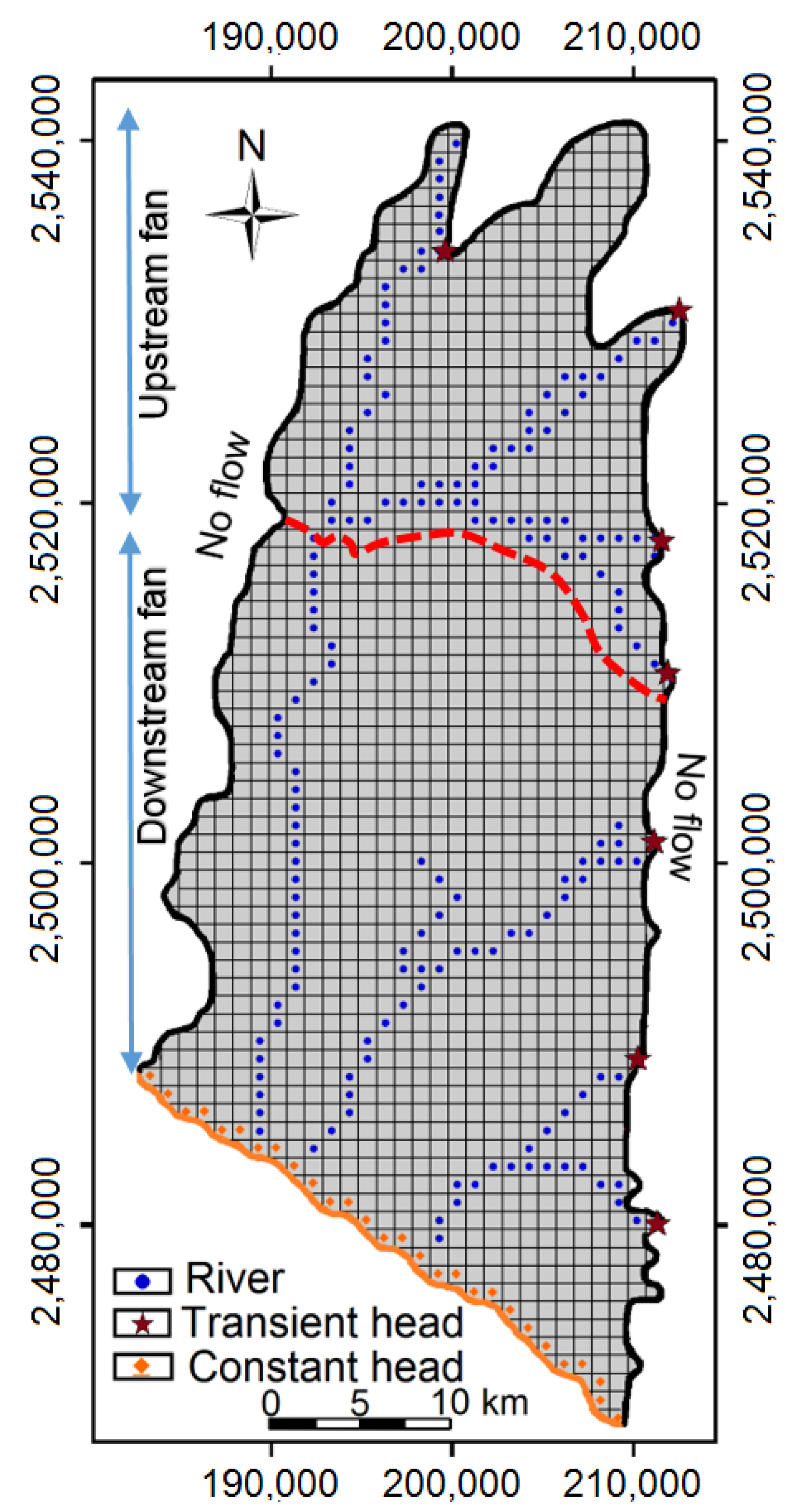
3.1. Conceptual Model and Parameters for Groundwater Flow

The reports of Taiwan CGS defined four aquifer layers with a total thickness of more than 200 m in the PPGB [22]. The groundwater monitoring network had shown a few interactions between the first layer and the deeper layers in the downstream fan area. Monitoring data also indicate that the first aquifer layer near the coastal line exhibits a good connection with the ocean. It is recognized that the topsoil influence and dominate the characteristics of the SGIs. In the PPGB, most pumping wells are installed in the first layer. In the study, the conceptual models then considered the first layer of the PPGB aquifer system for the simulations. The MODFLOW model used 40 rows and 90 columns with a uniform cell size of 1 × 1 km² for the entire PPGB (see Figure 4).

The transient flow simulations of MODFLOW-2005 involve 36 time steps ranging from 1 January 2015 to 31 December 2017. However, the time step of the MODFLOW in the GSFLOW simulations will become a day to resolve the daily variations of SGIs. In the MODFLOW model, the initial condition was specified based on the results of a steady-state simulation for the month of December in 2014. The steady-state model had been calibrated based on the monthly averaged data in December 2014, which is a month earlier than the starting time of the simulations. In the study, the altitude, topographic slope, and river network are distributed differently in the upstream and downstream fan areas. In the GSFLOW model, we considered two sub-watersheds to obtain the SGIs for upstream and downstream fan areas (see Figure 4). The upstream and downstream fan areas were divided based on the Li-lin Bridge. Note that the two sub-watersheds for upstream and downstream fan areas share the same groundwater model for the entire PPGB.

The MODFLOW-2005 model enables the consideration of different types of boundary conditions, including the default no-flow boundary condition, the specified hydraulic head boundary condition that can vary within or between stress periods, and the constant hydraulic head boundary condition that holds a fixed head value in all stress periods [14]. In the study, the hydrogeological boundaries for the entire PPGB domain are the western foothills, the northern low hills, the eastern mountain central range, and the southern Taiwan Strait. The no-flow boundaries are specified along the western foothill, the northern low hills, and the eastern central mountains. The boundary condition along the shoreline of the Taiwan Strait was the constant hydraulic head boundary condition. The specified hydraulic head boundaries are assigned to the inlet valleys of the rivers on the boundaries (see Figure 4). Note that the hydraulic head values at the river inlets used the observations of water levels from the nearest monitoring wells. Such specified hydraulic head boundary conditions allow assigning hydraulic head values that change over the simulation time steps. In the study, the aquifer thickness for the PPGB follows the definition of aquifer layers reported by Taiwan CGS [22]. In general, the aquifer thickness varies within the range of 60 to 100 m.

The river system in the study area consists of three main tributaries, namely the Kaoping River, the Tungkang River, and the Linpien River. All the rivers drain into the Taiwan Strait. Based on the definition of upstream and downstream fan areas in the study, the upstream of the Kaoping River (i.e., the northern segment of the Li-lin Bridge station) and along with the Aliao and Laonung Rivers form the upstream fan watershed (see Figure 1 and the dashed line in Figure 4 for the boundary). However, the downstream of the Kaoping River (i.e., the southern segment of the Li-lin Bridge station), the Tungkang River, and the Linpien River were included in the downstream fan watershed (see Figure 1 and Figure 4). In the study, the entire river system in the conceptual model of the PPGB was divided into 13 stream segments and 166 stream reaches. We fixed the streambed thickness of 3 m. In the PPGB, there are two streamflow stations Li-lin Bridge and Xing She Da Qiao. The Li-lin station monitors three main tributaries of the upper Kaoping, Laonung, and Ailiao Rivers. However, the Xing She Da Qiao station is on the Tungkang River. The time series of river flow observations were the basis for the GSFLOW model calibration and verification.

The basic hydrological parameters used in the simulation are the hydraulic conductivity and storage coefficients. In the study area, aquifer parameters had been obtained based on the hydraulic tests conducted during the development of the groundwater monitoring network [22]. Previous site investigations had recognized that the hydraulic conductivity varies significantly from 0.8 to 106 m/d in the PPGB. Most areas in the PPGB consist of gravel and sand deposits, and the values of hydraulic conductivity range from 70 to 80 m/d. Specifically, in the upstream fan area and some regions in the downstream fan areas, the values of hydraulic conductivity are within the interval of 90 to less than 110 m/d. These areas cover the upstream areas of the Kaoping River, the Laonung and Ailiao Rivers, and the upstream basins of the Tungkang and Linpien Rivers. In general, hydraulic conductivity values of 10 to 70 m/d occur along the downstream area of the Kaoping River [22]. Areas with low hydraulic conductivity values of the PPGB are in the lowland areas between the downstream Tungkang and Linpien Rivers. A typical anisotropic ratio of 1/10 was used in the study to account for the vertical hydraulic conductivity. Because the model considered one conceptual layer, the influence of the vertical hydraulic conductivity might be insignificant.

The unsaturated zone flow (UZF) package simulates the water flow from the soil zone to the saturated aquifer (i.e., below the groundwater level). In the MODFLOW model, the physical parameters in the UZF package play an essential role to account for the recharge from the surface water to the groundwater. In the study, the parameters such as the Brooks–Corey exponent in the UZF package, the saturated water content, and the initial unsaturated water content are 3.5, 0.25, and 0.2 [25]. The MODFLOW-2005 model uses the parameters in the UZF packages. However, in the GSFLOW simulation, parts of the UZF features in the MODFLOW have been replaced by the PRMS packages to estimate the detailed evapotranspiration and infiltration dynamics. In the study, we used the PEST module to calibrate the groundwater flow model. The calibration and validation relied on the GMS software environment. We found that PPGB-recharge and PPGB-pumping rates were the main sensitive parameters regarding model calibration.

3.2. Conceptual Model and Parameters for Surface Water Flow

In addition to the full model for the entire PPGB, the study further considered the PPGB as two different sub-regions (i.e., watersheds for upstream and downstream fans) based on the different flow patterns of the river network (see Figure 1 and Figure 4). These two sub-regions also reflect the long-term conditions of the landforms, especially the terrestrial slopes and land-use types. The following briefly describes the conceptual model and the associated modeling parameters for the PRMS model. In the GSFLOW model, the data consists of the daily maximal and minimal temperatures, precipitation, and streamflow for the period from 1 January 2015 to 31 December 2017. In the study, the number of MODFLOW-2005 cells for the aquifer layer is 3600, including active cells with 1327 and inactive cells declared in the dimension item. Note that the size of each cell is 1 × 1 km in the study. The stream segments and stream reaches were 13 and 166, respectively. The corresponding PRMS subsurface reservoirs include 17 hydrologic response units (HRUs) for the full PPGB model (see Figure 5). Note that the artificial recharge lake was assigned as the 18th HRU for the full basin model (Figure 5). The determination of the HRUs mainly depends on the properties such as the drainage boundary, land-surface altitude, land-surface slope, land use, and flow direction [11]. A watershed can include many HRUs. The study determined the HRUs by using the flow accumulation technique to define the boundaries of small watersheds. The small watersheds were then slightly modified to become the HRUs for the GSFLOW model. In the GSFLOW model, the parameters in each HRU can significantly influence the response of SGI for the HRU. Based on the available data for the study area, the simulations of the watershed responses considered the daily stress period for the three-years model. Other input parameters were integrated based on the observations from weather stations, land-use maps, and geology maps in the PPGB. With the limited observations, parts of dimensions and parameters might be assigned based on the default values used in previous investigations (e.g., [11]). The typical values associated with streamflow observations are the basis to conduct the trial and error calibration of the GSFLOW model.

Table 1. The ranges of the calibrated parameters for the groundwater and surface water flow (GSFLOW) model. Note that other parameters that are not on the list used the default values proposed by Markstrom et al. (2008) [11].

Parameter	Minimum Value	Maximum Value
fastcoef_lin	0.4	0.4
jh_coef	0.0024	0.004
pref_flow_den	0.4	0.4
smidx_coef	0.03	0.03
soil_moist_max	12	12
soil_rechr_max	6	6
ssr2gw_exp	0.5	0.5
ssr2gw_rate	0.2	0.2
wrain_intcp	0.05	0.05
smidx_exp	0.6	0.6
soil2gw_max	5	5
ssstor_init	10	10
rain_adj	1.76	5

lists the ranges of the calibrated parameters for the GSFLOW model. In the GSFLOW model, the calibration is based on the observations from the stream gauges and the regional groundwater network. Similar to the recharge calibration in the MODFLOW model, the transient pumping rates in the GSFLOW model were calibrated again with the data obtained from the local government because the available data was the year-averaged pumping volume.

4. Results and Discussion

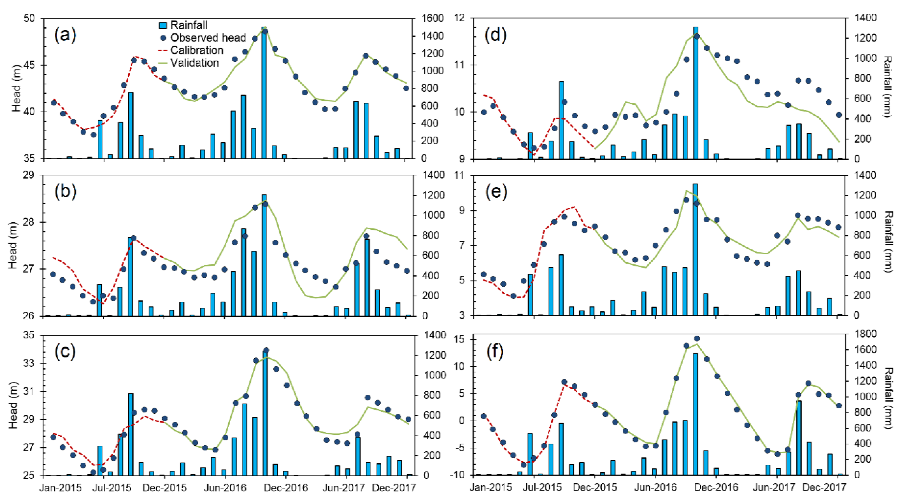
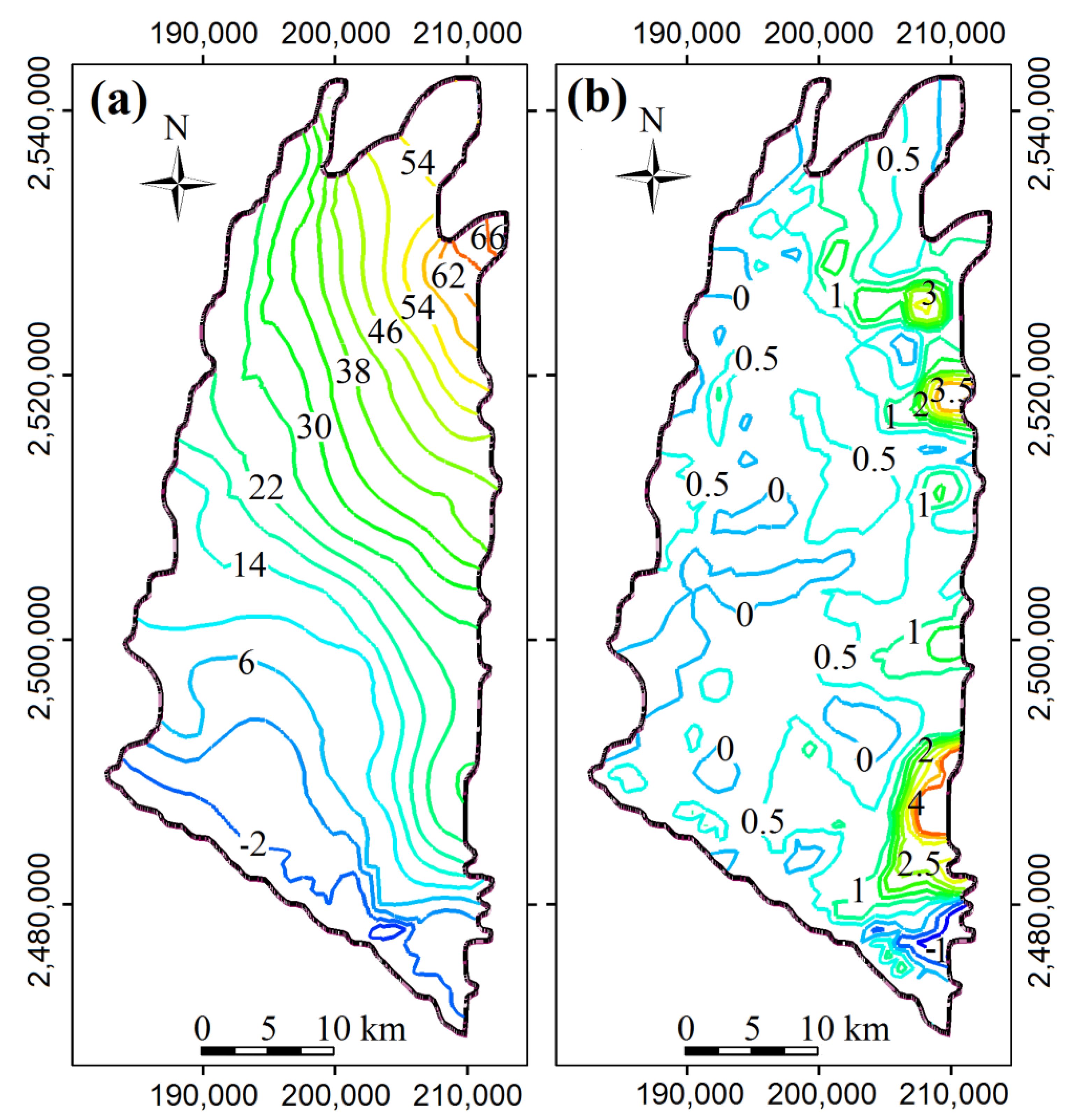
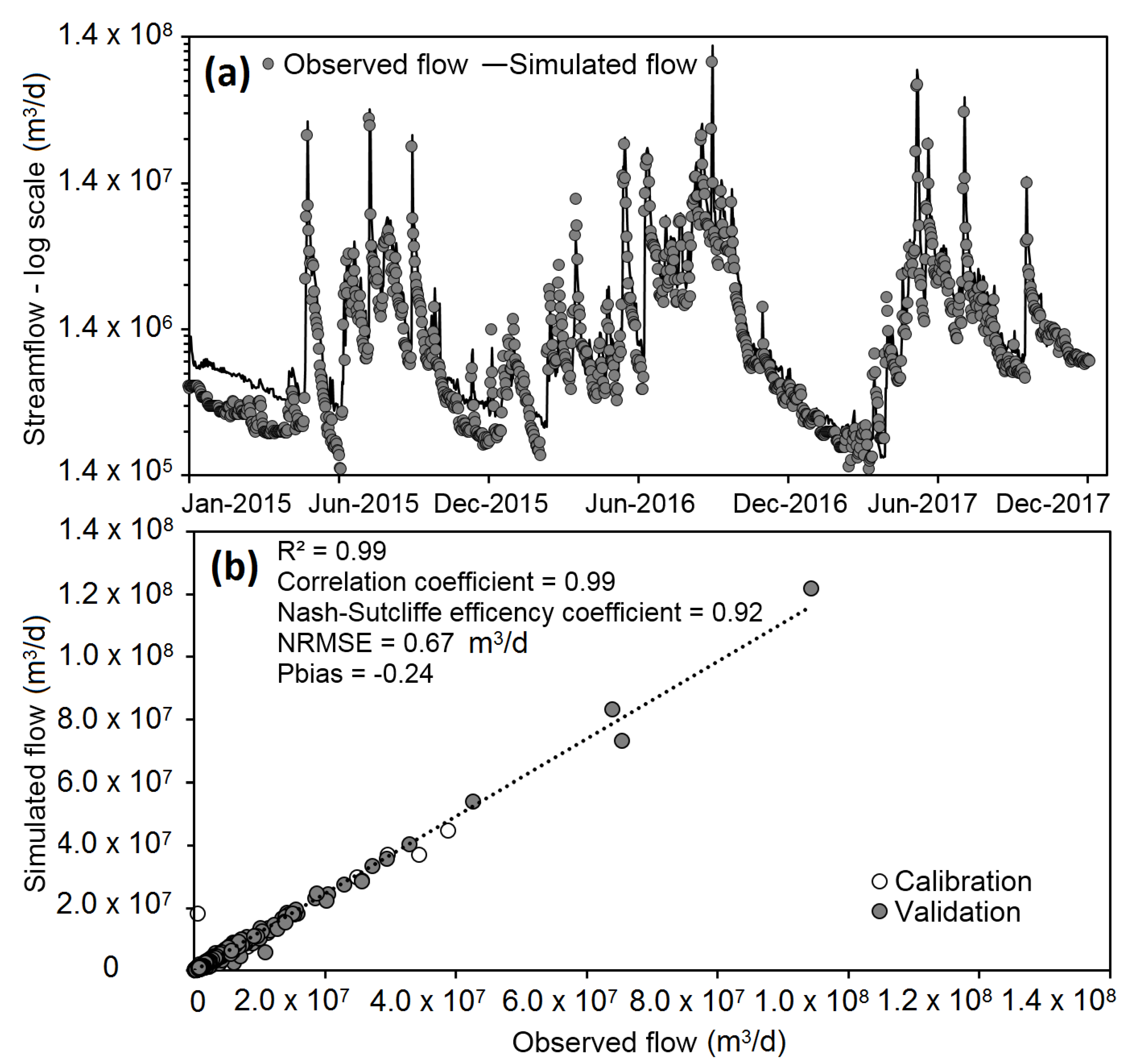
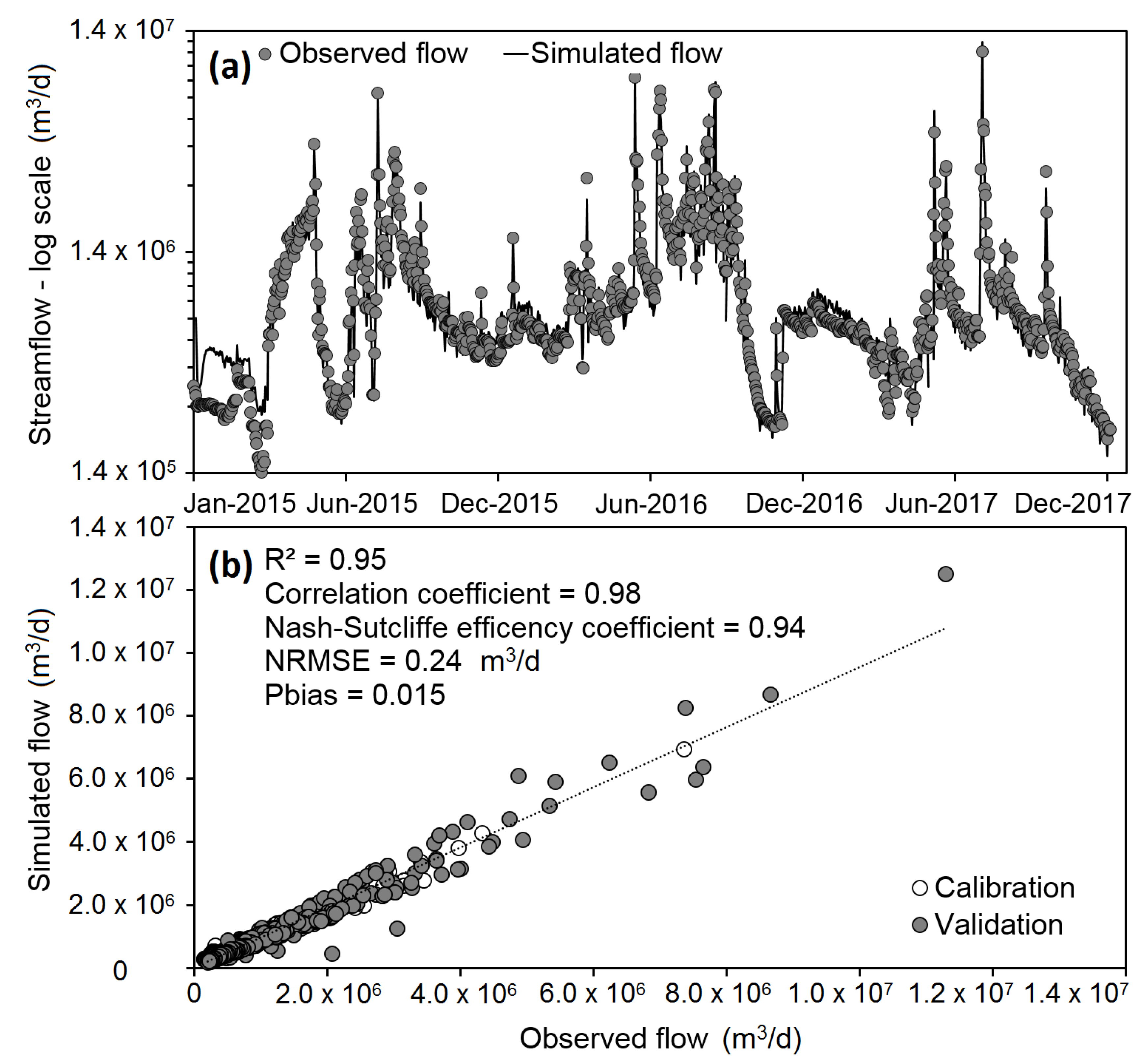
4.1. Model Calibration and Validation

Among the 39 observation wells, we selected six representative wells at different locations in the PPGB, namely Jiyang, Chiuju, Jianxing, Yongfang, Kanding, and Fangliao, to assess the spatio-temporal variations of the total hydraulic head. Figure 6 shows the results of the comparison for the selected wells. The calibration and validation periods have demonstrated that the coupled groundwater and surface water model can reproduce well the groundwater dynamics in the PPGB. The differences between the observed data and the simulated solution are limited to ±1 m. Note that the recharge and pumping rates are two sensitive parameters in the model and that these parameters are the main focus of the model calibration. In the study, the calibrated recharge and precipitation ratios for different cells were then used for the model validation. However, the variations of pumping rates were assumed to be the same through the validation periods.

We have shown that the substantial variations of the dry and wet seasons in the PPGB and the influence of precipitation on the groundwater variations are significant. Based on the precipitation data obtained from the PPGB, the period of the wet season is from May to October and the dry season is from November to the next April. The year 2016 was a wet year and had an extremely high total precipitation of 3796 mm. The plots of the monthly average rainfall considered the data from the weather stations that are closest to the monitoring wells. The dry and wet seasons led to groundwater variations of 2 to 20 m, depending on the locations of the monitoring wells. Such variations are significant in the downstream area (i.e., the Fangliao station, see Figure 6f). However, in the upstream area at the Jiyang station, the monitoring well shows the relatively mild variations of the groundwater levels as compared to other selected monitoring wells. The stations in the center area of the PPGB show small variations in groundwater levels. The small variations in groundwater levels might be relevant to the relatively high density of river branches. Note that the variations of groundwater levels are strongly influenced by the agriculture and aquaculture activities in the local areas. In the PPGB, the aquaculture pumping is highly active in the nearshore area.

The simulation results indicate that the high groundwater head regions are in the northeastern area near the Central Mountain Range of the PPGB. The hydraulic head values in these regions are higher than 60 m. In general, the groundwater levels gradually decrease from the northeastern area to the lower reaches of the Kaoping, Tungkang, and Linpien Rivers. In the downstream area in the basin lowland near the Taiwan Strait, the simulated hydraulic head values are less than 0 m because of the over-pumping of the groundwater along the coastal line (see Figure 7a). We found that the patterns of hydraulic head distributions for wet and dry seasons are nearly identical except for the small regions along the shoreline and near the confluence point at the Li-lin station. Figure 7b further shows the distribution of mean head differences in wet and dry seasons in the entire PPGB. Note that the calculations of hydraulic head differences are based on the cell-by-cell comparison of means of hydraulic heads for wet and dry seasons from 2015 to 2017. The results demonstrate that the significant differences of heads in wet and dry seasons are in the upstream areas of rivers in the PPGB. Figure 7b shows that the hydraulic head differences are similar along the rivers because the landforms and stream conditions in the model have significantly constrained the hydraulic head variations near the rivers. These areas with large hydraulic head differences are in the upstream zones of Kaoping, Laonung, and Ailiao Rivers. However, the highest variation of hydraulic heads in wet and dry seasons is in the upstream of the Linpien River. The averaged head differences can vary over 4 m, indicating the great environmental impact of wet and dry seasons on the groundwater variations. Additionally, the upstream areas of the Ailiao and Laonung River also show relatively high hydraulic head differences in wet and dry seasons. Such high groundwater variations are mainly induced by the considerable variations of topography in these upstream areas. These areas have been defined to be the recharge sensitivity zones for groundwater resource protection in the PPGB [26]. With the significant observation from previous investigations, an artificial recharge lake is therefore determined in the upstream area of the Linpien River to enhance the recharge and mitigate the impact of the over-pumping on the aquifer system near the coastal area. Assessing the effect of the anthropogenic construction on the interactions of groundwater and surface water will be presented later in the study.

Figure 8a and Figure 9a show the results of observed and simulated streamflow at the Li-lin Bridge and Xing She Da Qiao stations. Similar to the groundwater model, the calibration in the study considered the data obtained in the year of 2015. However, the validation process used the data obtained in 2016 and 2017. The comparison shows good agreement between the field observations and the solution from the GSFLOW model. The GSFLOW model resolves clearly the peak values and the small variations in wet and dry seasons through the simulation period. With a relatively larger drainage basin at the Li-lin Bridge station, the discharge rates of the Kaoping River at the Li-lin station are two orders of magnitude higher than those at the Xing She Da Qiao station. High variations of precipitation are the key factors that lead to significant variations in the streamflow. Figure 8b and Figure 9b further present the scatterplot for the data obtained from the field and the solution from model simulations. Based on the selected criteria to evaluate the accuracy of the simulations, we obtained high correlations for the surface water flows at the Li-lin Bridge and Xing She Da Qiao stations. The coefficient of determination (R²) for the Li-lin Bridge station is 0.99 and a slightly small value of 0.95 is obtained for the Xing She Da Qiao station. Coefficients of correlation (RE) values are 0.99 for the Li-lin Bridge station and 0.98 for the Xing She Da Qiao station. Using the Nash-Sutcliffe efficiency coefficient (NSE) to evaluate simulation results shows that the results at the Xing She Da Qiao station have better performance than those at the Li-lin Bridge station. The NSE values are 0.92 and 0.94 for the Li-lin Bridge and Xing She Da Qiao stations, respectively. Besides that, the calculated normalized root-mean-square errors (NRMSE) showed different results for the two selected streamflow stations. In detail these NRMSE’s were 0.67 for the Li-lin Bridge and 0.24 for the Xing She Da Qiao stations. The percent bias (Pbias) aims to evaluate the average tendency of the simulated values to be larger or smaller than their observed ones. In the study, the Pbias values for the Li-lin Bridge and Xing She Da Qiao stations are −0.24 and 0.015 for the model validation, indicating that the modeling results at the Li-lin station tend to underestimate the observations. However, the results at the Xing She Da Qiao station slightly overestimate the streamflow.

Figure 10 further shows the variations of the discharge rates obtained from the GSFLOW model. The daily averaged outflows from the rivers are 2.5 million m³/d for the Kaoping River, 1.3 million m³/d for the Tungkang River, and 0.5 million m³/d for the Linpien River. However, the variations of discharge rates for the Kaoping River in dry and wet seasons are extremely high as compared with those for the Tungkang and Linpien Rivers. The flow rates of the Kaoping River in the dry and wet seasons can vary in three orders of magnitude. The relatively large watershed might induce the high variations of flow rates as compared with the watersheds of the other two rivers. Notice that there is no stream station at the outlets of the rivers. In the study, the results have solely relied on the results obtained from the calibrated GSFLOW model.

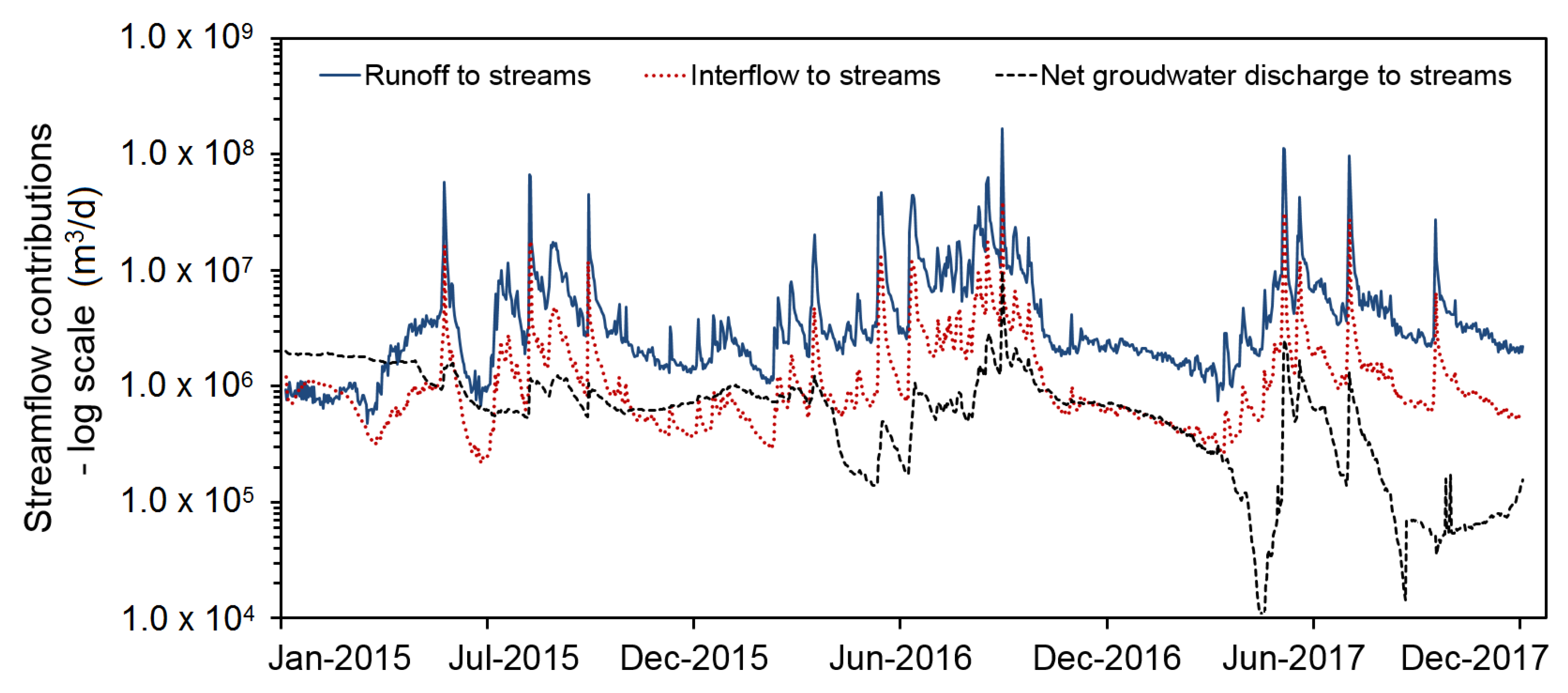
4.2. Surface Water and Groundwater Interactions

The proposed numerical model has shown results that agree well with the surface water and groundwater observations in the PPGB. Specifically, the one-year calibration and two-years validation periods were conducted to ensure the accuracy of the model. The following sections focus on addressing the essential issues of SGIs in the study area. The results and discussions are based on the model outputs that cover the simulations from January 2015 to December 2017.

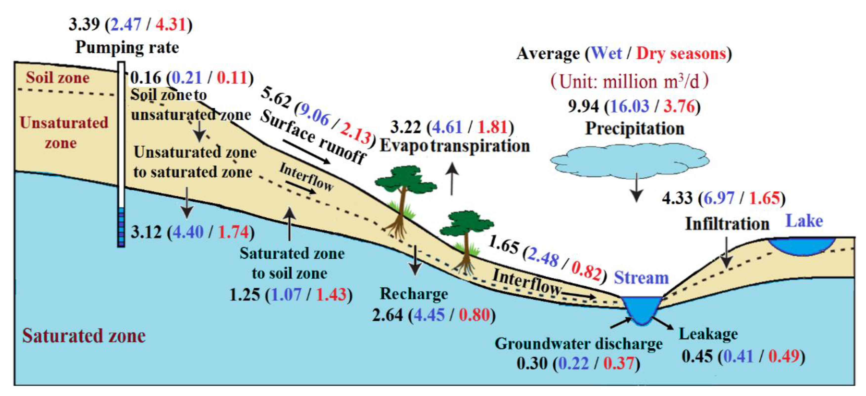
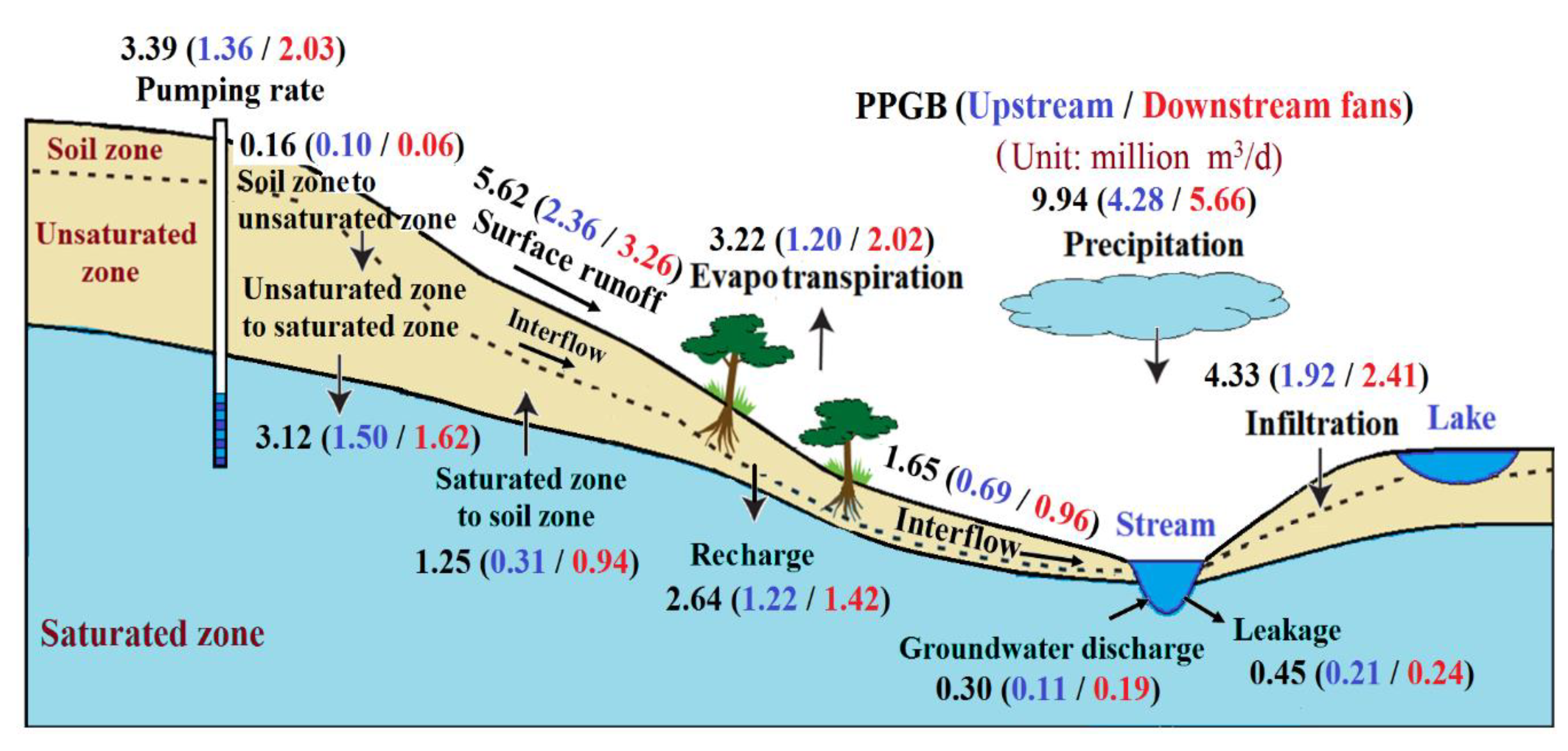
4.2.1. Water Cycle for the Entire PPGB

Table 2. The statistics of the groundwater budgets that were obtained from the MODFLOW in the GSFLOW model.

Sources/Sinks	In (m3/d)	Out (m3/d)	STDin (m3/d)	STDout (m3/d)
Storage	3.96 × 106	2.00 × 105	1.86 × 106	2.19 × 105
Constant head	1.12 × 105	1.74 × 105	9.68 × 104	2.09 × 105
Wells	0	3.43 × 106	0	1.38 × 106
UZF recharge	2.13 × 105	0	2.88 × 105	0
GW Evapotranspiration	0	2.32 × 104	0	3.42 × 104
Surface leakage	0	5.44 × 105	0	6.30 × 105
Stream leakage	3.53 × 105	2.75 × 105	1.19 × 105	3.61 × 105
Total	4.64 × 106	4.64 × 106	1.79 × 106	1.79 × 106
In-Out	−8.77 × 102
Percent Discrepancy	−1.97 × 10−2

summarizes the cell-by-cell water budgets of the groundwater model for the entire PPGB. The results in Table 2 also present the statistics of the groundwater budgets obtained from the calibrated GSFLOW model during the three-year simulation period. The numerical model shows the mass conservation for the groundwater system because of the small value of the percent discrepancy. An order of magnitude difference was obtained for the cell-by-cell “storage in” and “storage out” for the simulation domain. In the study, we specified the constant hydraulic head boundaries at the upstream valleys of the rivers and along the coastal line. Results in Table 2 have indicated that the average flow rate along the coastal line is slightly larger than the flow rates along the inlets near the upstream valleys. The flow rate variations (i.e., the standard deviation (STD) of the flow rates) along the coastal line are also slightly higher than those along the inlets near the upstream valleys. The GSFLOW model enables the calculation of detailed processes involved in the water cycle. Specifically, the surface dynamics have been resolved with more water budget components in the PRMS model. Figure 11 summarizes the fluxes of different water cycle components in the PPGB. Note that the wet season was defined from May to October for each year, and the dry season was collected from November to April in the next year. We have focused on the interaction dynamics between the surface water and the first layer of the groundwater system. To verify the flow from the unsaturated zone to the saturated zone from the output of the GSFLOW model, the calculation of groundwater recharge relies on the available results of water budget components in the PRMS. These components include the precipitation, evapotranspiration, surface runoff, soil infiltration, interflow to streams, stream leakage to saturated and unsaturated zones, groundwater discharge to streams, gravity drainage from soil zones to unsaturated zones, recharge from unsaturated zones to saturated zones, and groundwater discharge from the saturated zones to soil zones. In the study, the groundwater recharge in the GSFLOW was manually calculated by subtracting the flow rates of evapotranspiration, surface runoff, and interflow from the flow rate of the total precipitation.

The results of the water budgets show that the main input (i.e., precipitation) in the water cycle is 9.94 × 10⁶ m³/d, which is accounted for 3.6 × 10⁹ m³ on average in a year (see Figure 11). The discrepancy of the precipitation in wet and dry seasons is extremely high. Over 80% of the precipitation is from the wet season. With the relatively open area and gravel deposit on the land surface, the average infiltration is approximately 40% of the average precipitation and the average surface runoff is about 57% of the average precipitation. In the PPGB, the volumetric flux of the evapotranspiration is 3.22 × 10⁶ m³/d. This evapotranspiration value obtained from the GSFLOW model comprises the evaporation of intercepted precipitation, the evapotranspiration from the unsaturated and saturated zones, and the evapotranspiration from HRUs. Note that the GSFLOW model has modified the features of the UZF package in the MODFLOW model. The volume is accounted for 1.2 × 10⁹ m³ on average in a year. The water from the soil zone to the unsaturated zone is involved in the overall behavior of the infiltration. In the PPGB, the volumetric flux from the soil zone to the unsaturated zone (i.e., 0.16 × 10⁶ m³/d) is 4% of the total average infiltration (i.e., 4.33 × 10⁶ m³/d). In the PRMS, calculating infiltration depends on the precipitation rate, surface runoff, and soil material. In the study, we obtained similar ratios of water fluxes from wet and dry seasons for the precipitation, surface runoff, and infiltration. With the available results from the GSFLOW, it is possible to calculate the detailed sources of different components in the water cycle. However, the post-processing is required to extract the solution from the GSFLOW model. The surface runoff contributes approximately 77% and 64% of the streamflow for wet and dry seasons. The interflow provides 21% and 25% of the streamflow in the wet and dry seasons. The groundwater discharge has relatively small contributions to the streamflow. The percentages are 2% and 11% in the wet and dry seasons. Based on the observations from streamflow stations in the PPGB, the variations of streamflow in wet and dry seasons can vary up to three orders of magnitude differences. The small percentage of groundwater discharge to the streamflow can be significant for the dry seasons.

The components “stream leakage to unsaturated and saturated zones” and “groundwater discharge to streams“ are the indicators that show the local dynamics of streams and groundwater interactions. Simulation results show that the flux of stream leakage is relatively higher than the flux of groundwater discharge. We also found that the average discharge of groundwater to streams is noticeable in wet (0.22 × 10⁶ m³/d) and dry (0.37 × 10⁶ m³/d) seasons. However, the differences between groundwater discharge to stream and stream leakage to groundwater are similar in wet and dry seasons. We found that the interflow in the water cycle plays an important role in the river system in the entire PPGB. The interflow rate is approximately 1.65 × 10⁶ m³/d on average. In the wet seasons, the flux of the interflow rate is 200% more than the dry seasons. A large amount of interflow had motivated a different type of water usage in many areas near the rivers. In the PPGB, many underground channels were built along or partially cross the streams to collect the interflow water. Much of the irrigation and consumption water is from the interflow. Practical operations have shown that the interflow water resource is relatively stable as compared to the water directly obtained from the streams. The quality of the interflow water is also better because the natural underground deposits can be the low-level filters that reduce the water turbidity. This feature supports the important water resources in flooding seasons because of the high turbidity of the river water in storm events.

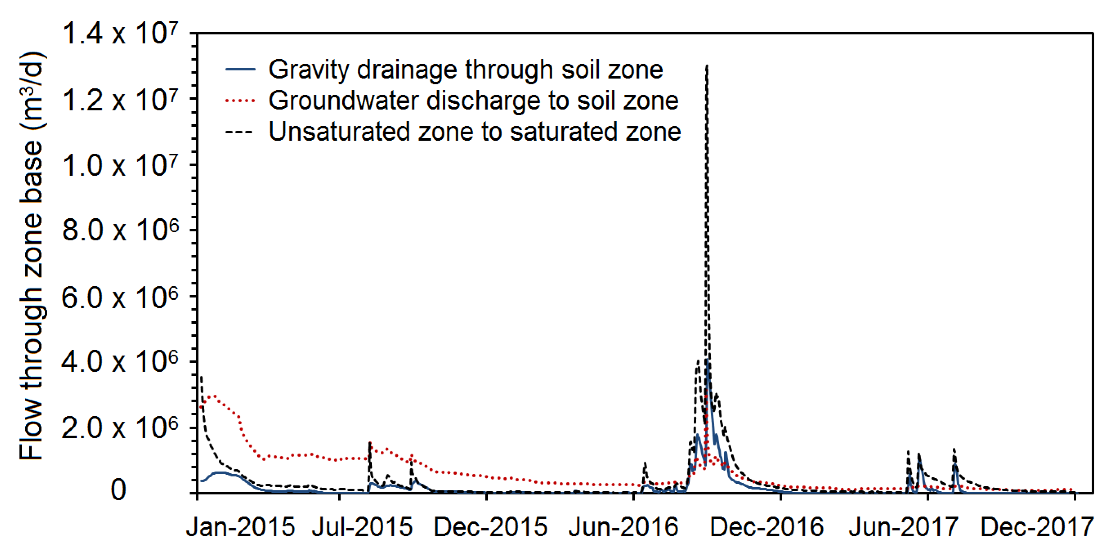
4.2.2. Seasonal Variations of the SGIs and Interactions Near the Soil Zones

The precipitation is the primary input for a regional water cycle. The budgets of the water cycle components are useful for evaluations of watershed sustainability. However, the percentages of water budgets might not be sufficient for water resources management for most practical problems. Previous investigations have shown that the temporal variations of the water budget are crucial for efficient water resources management. The temporal variations are essential for areas with highly nonuniform precipitation, complex land-use, and anthropogenic activities. In the study, the model outputs allow the assessment of detailed variations near the interface of surface water and groundwater. We are interested in the temporal variations of SGIs. Specifically, two interfaces, including the saturated zones near stream beds and unsaturated zones near the soil layer, were considered to quantify the dynamics of the interactions.

The main supplies of the rivers in the PPGB include surface runoff, interflow, and groundwater discharge to the stream. Figure 12 shows the temporal variations of three main components that contribute to streams. In general, the surface runoff in the PPGB provides 70% of the streamflow. The interflow offers approximately 20% volumetric flow to the streamflow. Only 10% of water is from net groundwater discharge to streams. The map of the water cycle shows that rainfall is the main factor that influences the streamflow. The temporal variations of interflow are similar to those of the surface runoff and precipitation. However relatively small values of net groundwater discharge to streams were obtained for the PPGB. The differences between the surface runoff and net groundwater discharge to streams vary significantly through a year. Note that the net groundwater discharge to streams is calculated by subtraction of the surface runoff and interflow from the streamflow. Investigations have recognized that the net groundwater discharge to streams is an important source of stream base flow. In the dry seasons, the volumetric water in streams is critical to fit the ecological conditions. The daily values of the net groundwater discharge to streams are relatively small and highly variable in recent years. Human activities such as groundwater pumping might be the main factors that directly influence the variations of net groundwater discharge to streams. To improve the groundwater environment, the increase of the groundwater levels might be required to enhance the net groundwater discharge to streams in the PPGB. In the PPGB, we have obtained a relatively high potential of the water resource from interflow. However, the spatial variation of the interflow along streams is not available because of the model limitations.

On the interface near the soil and unsaturated zones, there are three components considered in the GSFLOW model. These three components, including soil zone, unsaturated zone, and saturated zone, might have interactions between two of them. The fluxes near the interface are gravity drainage from the soil zone to the unsaturated zone, recharge from the unsaturated zone to the saturated zone, and groundwater discharge from the saturated zone to the soil zone, respectively. Note that the condition that the groundwater discharge into the soil zone is that the groundwater head in a connected finite-difference cell is higher than the soil zone base. In Figure 13, we have extracted the temporal variations of different total fluxes from January 2015 to December 2017. The volumetric flow rates of the groundwater discharge to the soil zone are relatively high in the PPGB. Nearly identical fluxes were obtained for the recharge from the unsaturated zones to the saturated zones and the gravity drainage from the soil zones to the unsaturated zones. The gravity drainage to the unsaturated zones and the recharge from the unsaturated to the saturated zones are highly sensitive with the variations of rainfall. Note that the results in Figure 13 only provide the overall performance of the system responses for different components. In the study, the GSFLOW model accumulates the results from HRUs in the PPGB. The spatial variations might be limited by the sizes and shapes of the HRUs defined in the model.

4.2.3. The Behavior of the Interactions in the Upstream and Downstream Fans

The PPGB is a relatively large area with high variations of altitude and slope and a complex river network. The natural processes such as tectonic deformation, surficial deposition, and human activities have led to different behaviors of SGIs in the upstream and downstream fan areas in the PPGB. Figure 14 shows the average volumetric flow rates for the water cycle components obtained from the GSFLOW model. In the study, we had defined the upstream fan in the upstream area of the confluence point (i.e., the Li-lin Bridge) of the Kaoping River in the PPGB. However, the remanding area in the PPGB was defined as the downstream fan area that includes the downstream area of the Li-lin Bridge station and covers the Tungkang and Linpien Rivers in the PPGB. We are interested in understanding the behavior of SGIs and quantifying the water cycle that had been influenced by the natural processes and human activities.

The water budgets in Figure 14 indicate that the average volumetric flow rates in the downstream fan area are generally higher than those in the upstream fan area. In the upstream fan area, only the average flow rate of the soil zone to the unsaturated zone is higher than that in the downstream fan area. The observations of the precipitation from 2015 to 2017 show that the upstream fan received relatively less average precipitation as compared to the data obtained from the downstream fan area (see Figure 14). However, the relatively high permeability of topsoil in the upstream fan can lead to the high flux of the vertical flow from the soil zones to the unsaturated zones. In Figure 14, the averaged water fluxes accumulate the fluxes from all computational cells in the simulation. By counting the water fluxes for the unit area in the upstream or downstream fans, we obtained relatively substantial interactions of the water cycle in the upstream fan area. Such interactions are very obviously near streams and indicate high impacts between groundwater and surface water systems in the upstream fan area.

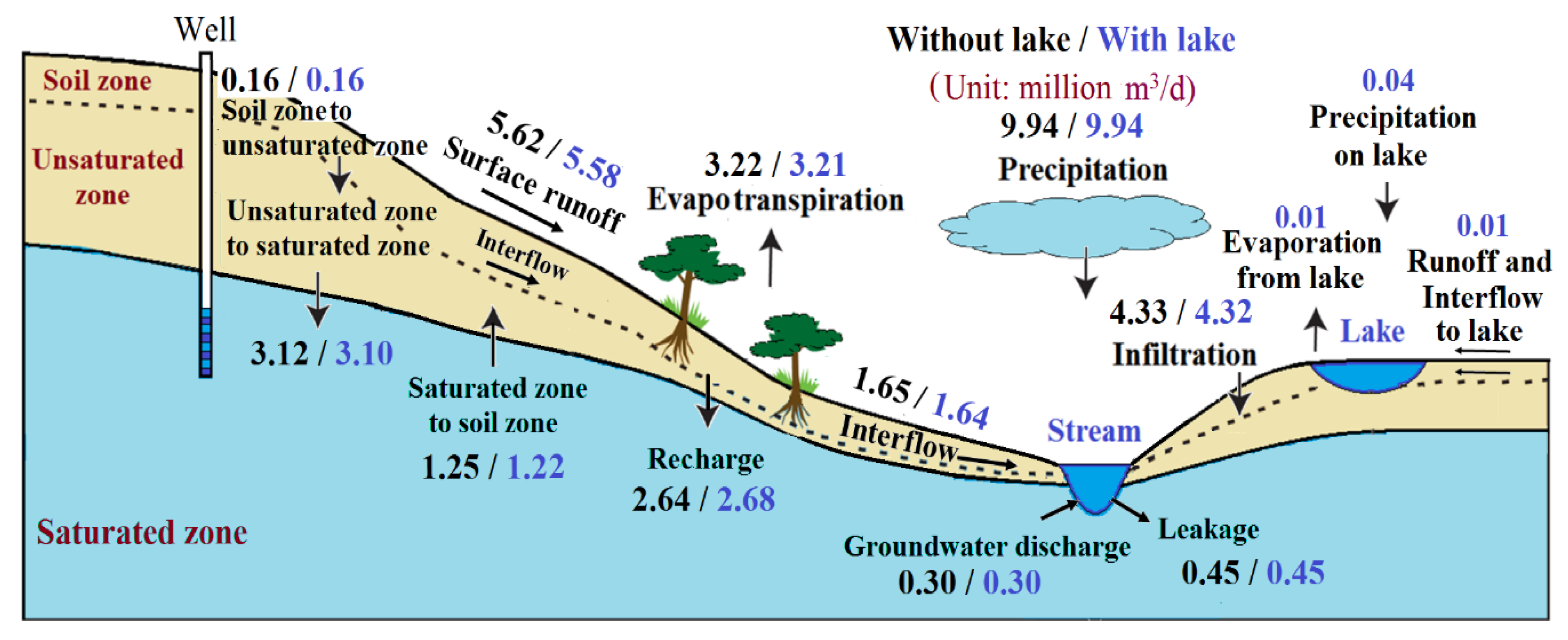
4.2.4. Effects of the Artificial Recharge on the Local Water Cycle

The flow directions of the Kaoping, Tungkang, and Linpien Rivers are generally in a north-south direction to the Taiwan Strait in the downstream fan area. With the intensive developments of aquaculture and agriculture industries, the downstream fan area had faced severe problems of groundwater over-pumping and groundwater contamination [20]. An artificial recharge project was proposed recently to mitigate the impact of over-pumping near the coastal area. The artificial lake with a total area of approximately 3 km² was planned to be located in the upstream region of the Linpien river (see 18th HRU in Figure 5). This area is the same as the determined zone with the highest head differences in wet and dry seasons (see Figure 7b). The operations of the artificial lake in the model follow the designed strategies. In the GSFLOW model, the initial stage was 40 m, specified based on the averaged local altitude near the artificial lake. The operation of the lake stages varies from 34 to 51 m, depending on the river stages. Scenarios with and without the artificial lake were considered to quantify the effect of the artificial lake on the local SGIs. Note that the cases for the comparison used the full PPGB for the modeling domain. In the GSFLOW model, the case without the lake did not have the 18th HRU, while the case with the lake added the 18th HRU in the simulation domain. The study used the lakebed hydraulic conductivity the same as the streambed hydraulic conductivity in the stream cells. Other parameters such as the precipitation in the lake area and evaporation from the lake are the same as those in the case without the artificial lake.

There are additional terms in the water cycle for the case with the artificial lake. We exported the results from the GSFLOW model and presented the water fluxes in Figure 15. Because the lake has a relatively small area as compared to the entire PPGB, the contribution of the artificial lake on the water budgets is insignificant. For the cases with and without the lake, we had fixed the simulation conditions and the associated hydrogeological parameters. The slightly different fluxes in the water cycle can be considered as the effect of the artificial lake on the regional water budgets. Simulation results show that the lake can reduce the direct infiltration, surface runoff, and interflow because the land area had been replaced by the artificial recharge lake (see Figure 15). The influence of the artificial lake on the SGIs near streams is insignificant. Such a result indicates the small impact of the artificial recharge lake on the surface water environment. In the study, the case with the lake shows that the component of the averaged groundwater recharge increases 0.04 × 10⁶ m³/d, which is approximately 1.46 × 10⁷ m³ in a year. The result of groundwater recharge is based on the available water budget components in the PRMS. The dynamics of the interactions in the local area might need smaller scales of HRUs and the associated observations to validate the model.

5. Conclusions

The objectives of the study are to characterize the behavior of SGIs in the PPGB and quantify the influence of such interactions induced by the landforms and anthropogenic activities. The interactions between surface water and groundwater have been assessed based on the GSFLOW model. The study conducts model calibration and validation by using observations from January 2015 to December 2017. The influences of wet and dry seasons on the SGIs are quantified based on the calibrated and validated model. An artificial recharge lake located in the upstream region of the Linpien River is assessed to quantify the impact of the water resource infrastructure on the local water cycle.

Results of calibration and validation have demonstrated that the coupled groundwater and surface water model can reproduce well the dynamics of the water interactions in the PPGB. Calibration results show that the differences between observed groundwater data and simulated solutions are limited to ±1 m. Simulations also show good agreement between the river flow observations and the solutions from the GSFLOW model. In general, the dry and wet seasons yield groundwater levels varying from 2 to 20 m. The groundwater variations are significant in the downstream area of the PPGB. The substantial differences in groundwater levels in the wet and dry seasons are obtained in the river upstreams in the PPGB. The differences of the averaged hydraulic heads in the wet and dry seasons can vary over 4 m, indicating the high impact of the wet and dry seasons on the groundwater variations.

The water budgets show that over 80% of the precipitation is from the wet seasons in the PPGB. The average infiltration is approximately 40% of total precipitation, and the surface runoff is about 57% of the total precipitation. The water from the soil zones to the unsaturated zones is involved in the overall behavior of the infiltration. In the PPGB, the volumetric flux from the soil zones to the unsaturated zones is 4% of the total infiltration on average. The surface runoff, interflow, and net groundwater discharge provide approximately 70%, 20%, and 10% volumetric flow to the streamflow, respectively. The interflow in the water cycle plays an essential role in the river system in the entire PPGB. The average interflow rate is approximately 1.65 × 10⁶ m³/d. The flux of the interflow rate in the wet seasons is 200% more than that in the dry seasons. In the PPGB, a large amount of interflow has motivated a different type of water usage in many areas near the rivers.

The average flow rates of most water cycle components in the downstream fan area are higher than those in the upstream fan area. In the upstream fan area, only the average flow rate of the soil zones to the unsaturated zones is higher than that in the downstream fan area. The observations of the precipitation from 2015 to 2017 have shown that the upstream fan received relatively less average precipitation as compared to the data obtained for the downstream fan area. However, the relatively high permeability of topsoils in the upstream fan can lead to the high flux of the vertical flow from the soil zones to the unsaturated zones. By counting the performance of water fluxes for the unit area, we obtain relatively strong interactions of the water cycle in the upstream fan area. Such interactions are obviously near rivers and indicate high impacts between groundwater and surface water systems in the upstream fan area.

In the study, the case with an artificial recharge lake is represented by an additional HRU in the GSFLOW model. Because of the relatively small area, the contribution of the recharge lake on the water budgets is insignificant. Simulation results show that the lake can reduce the direct infiltration, interflow, and surface runoff because the artificial recharge lake has replaced the land area. There is no influence of the artificial lake on the SGIs near streams, indicating the small impact of the artificial recharge lake on the surface water environment. Understanding the differences between the simulated and the designed groundwater recharge might require advanced investigations to modify the model. With limited field observations for the GSFLOW model, future studies might consider the uncertainty analyses to quantify the effects of the parameter uncertainty or natural heterogeneity on the interactions of surface water and groundwater. However, sufficient data should be obtained to develop the geostatistical structures for the parameters.

References

1. Yang, Z.; Zhou, Y.; Wenninger, J.; Uhlenbrook, S.; Wang, X.; Wan, L. Groundwater and surface-water interactions and impacts of human activities in the Hailiutu catchment, northwest China. Hydrogeology 2017, 25, 1341–1355. [Google Scholar] [CrossRef]
2. Lekula, M.; Lubczynski, M.W. Use of remote sensing and long-term in-situ time-series data in an integrated hydrological model of the Central Kalahari Basin, Southern Africa. Hydrogeology 2019, 27, 1541–1562. [Google Scholar] [CrossRef] [Green Version]
3. An, H.; Yu, S. Finite volume integrated surface-subsurface flow modeling on non-orthogonal grids. Water Resour. Res. 2014, 50, 2312–2328. [Google Scholar] [CrossRef]
4. Wei, X.; Bailey, R.T. Assessment of system responses in intensively irrigated stream-aquifer systems using SWAT-MODFLOW. Water 2019, 11, 1576. [Google Scholar] [CrossRef] [Green Version]
5. Kuffour, B.N.; Engdahl, N.; Woodward, C.; Condon, L.; Kollet, S.; Maxwell, R. Simulating coupled surface-subsurface flows with ParFlow v3.5.0: Capabilities, applications, and ongoing development of an open-source, massively parallel, integrated hydrologic model. Geosci. Model Dev. 2020, 13, 1373–1397. [Google Scholar] [CrossRef] [Green Version]
6. Panday, S.; Huyakorn, P.S. A fully coupled physically-based spatially-distributed model for evaluating surface/subsurface flow. Adv. Water Resour. 2004, 27, 361–382. [Google Scholar] [CrossRef]
7. Muma, M.; Rousseau, A.N.; Gumiere, S.J. Assessment of the impact of subsurface agricultural drainage on soil water storage and flows of a small watershed. Water 2016, 8, 326. [Google Scholar] [CrossRef] [Green Version]
8. Brunner, P.; Simmons, C.T. HydroGeoSphere: A fully integrated, physically based hydrological model. Ground Water 2012, 50, 170–176. [Google Scholar] [CrossRef] [Green Version]
9. Salem, A.; Dezső, J.; El-Rawy, M.; Lóczy, D. Hydrological modeling to assess the efficiency of groundwater replenishment through natural reservoirs in the Hungarian Drava River floodplain. Water 2020, 12, 250. [Google Scholar] [CrossRef] [Green Version]
10. El-Rawy, M.; Zlotnik, V.A.; Al-Raggad, M.; Al-Maktoumi, A.; Kacimov, A.; Abdalla, O. Conjunctive use of groundwater and surface water resources with aquifer recharge by treated wastewater: Evaluation of management scenarios in the Zarqa River Basin, Jordan. Environ. Earth Sci. 2016, 75, 1146. [Google Scholar] [CrossRef]
11. Markstrom, S.L.; Niswonger, R.G.; Regan, R.S.; Prudic, D.E.; Barlow, P.M. GSFLOW Coupled Groundwater and Surface-Water Flow Model Based on the Integration of the Precipitation Runoff Modeling System (PRMS) and the Modular Groundwater Flow Model (MODFLOW-2005); U.S. Geological Survey Techniques and Methods 6-D1; U.S. Geological Survey: Reston, VA, USA, 2008; p. 240. Available online: https://pubs.usgs.gov/tm/tm6d1/pdf/tm6d1.pdf (accessed on 13 October 2020).
12. Shu, Y.; Li, H.; Lei, Y. Modelling groundwater flow with MIKE SHE using conventional climate data and satellite data as model forcing in Haihe Plain, China. Water 2018, 10, 1295. [Google Scholar] [CrossRef] [Green Version]
13. Arnold, J.G.; Kiniry, J.R.; Srinivasan, R.; Williams, J.R.; Haney, E.B.; Neitsch, S.L. Soil and Water Assessment Tool Input/Output File Documentation Version 2009; Texas Water Resources Institute Technical Report No. 365; Texas A&M University System: College Station, TX, USA, 2011; Available online: https://swat.tamu.edu/media/19754/swat-io-2009.pdf (accessed on 13 October 2020).
14. Harbaugh, A.W. MODFLOW-2005, The U.S. Geological Survey Modular Groundwater Model—The Groundwater Flow Process; USGS Techniques and Methods 6-A16; USGS: Reston, VA, USA, 2005. Available online: https://doi.org/10.3133/tm6A16 (accessed on 13 October 2020).
15. Leavesley, G.H.; Lichty, R.W.; Troutman, B.M.; Saindon, L.G. Precipitation Runoff Modeling System; User’s Manual; USGS Water Resources Investigations Report 83-4238; USGS: Denver, CO, USA, 1983. Available online: https://doi.org/10.3133/wri834238 (accessed on 13 October 2020).
16. McCallum, A.M.; Andersen, M.S.; Giambastiani, B.M.S.; Kelly, B.F.J.; Ian Acworth, R. River aquifer interactions in a semi-arid environment stressed by groundwater abstraction. Hydrol. Process. 2013, 27, 1072–1085. [Google Scholar] [CrossRef]
17. Wu, B.; Zheng, Y.; Wu, X.; Tian, Y.; Han, F.; Liu, J.; Zheng, C. Optimizing water resources management in large river basins with integrated surface water-groundwater modeling: A surrogate-based approach. Water Resour. Res. 2015, 51, 2153–2173. [Google Scholar] [CrossRef]
18. Joo, J.; Tian, Y.; Zheng, C.; Zheng, Y.; Sun, Z.; Zhang, A.; Chang, H. An integrated modeling approach to study the surface water-groundwater interactions and influence of temporal damping effects on the hydrological cycle in the Miho catchment in South Korea. Water 2018, 10, 1529. [Google Scholar] [CrossRef] [Green Version]
19. Suppe, J. Kinematics of arc-continental collision, flipping of subduction, and back-arc spreading near Taiwan. Mem. Geol. Soc. China 1984, 6, 21–33. [Google Scholar]
20. Vu, T.D.; Ni, C.F.; Li, W.C.; Truong, M.H. Modified index-overlay method to assess spatial-temporal variations of groundwater vulnerability and groundwater contamination risk in areas with variable activities of agriculture developments. Water 2019, 11, 2492. [Google Scholar] [CrossRef] [Green Version]
21. Ting, C.S.; Zhou, Y.X.; De Vries, J.J.; Simmers, I. Development of a preliminary groundwater flow model for water resources management in the Pingtung Plain, Taiwan. Ground Water 1997, 36, 20–36. [Google Scholar] [CrossRef]
22. Taiwan, C.G.S. Hydrogeological Survey Report of Pingtung Plain, Taiwan; Central Geological Survey Ministry of Economic Affairs Executive Yuan: Taiwan, 2002; pp. 97–142.
23. Leavesley, G.H.; Restrepo, P.J.; Markstrom, S.L.; Dixon, M.; Stannard, L.G. The Modular Modeling System (MMS): User’s Manual; U.S. Geological Survey Open-File Report 96-151; U.S. Geological Survey: Denver, CO, USA, 1996. Available online: https://pubs.usgs.gov/of/1996/0151/report.pdf (accessed on 13 October 2020).
24. Niswonger, R.G.; Prudic, D.E.; Regan, R.S. Documentation of the Unsaturated-Zone Flow (UZF1) Package for Modeling Unsaturated Flow between the Land Surface and the Water Table with MODFLOW-2005; U.S. Geological Survey Techniques and Methods 6-A19; U.S. Geological Survey: Reston, VA, USA, 2006; p. 74. Available online: https://pubs.usgs.gov/tm/2006/tm6a19/pdf/tm6a19.pdf (accessed on 13 October 2020).
25. Brooks, R.H.; Corey, A.T. Properties of porous media affecting fluid flow. Irrig. Drain. Div. 1966, 92, 61–88. [Google Scholar]
26. Liang, C.P.; Jang, C.S.; Liang, C.W.; Chen, J.S. Groundwater vulnerability assessment of the Pingtung plain in Southern Taiwan. Int. J. Environ. Res. Public Health 2016, 13, 1167. [Google Scholar] [CrossRef] [PubMed] [Green Version]
Publisher’s Note: MDPI stays neutral with regard to jurisdictional claims in published maps and institutional affiliations.
Figure 1. The study area and the selected hydrogeological profiles: (a) the Pingtung Plain groundwater basin (PPGB) and the monitoring stations for surface water and groundwater, (b) the geological profile for cross-section b1-b5, and (c) the geological profile for cross-section a-a’. Note that the area in the upstream of the confluence point (i.e., Li-lin Bridge) of the Kaoping river, Ailiao, and Laonung rivers was defined as the upstream fan in the study. The downstream area of the Kaoping river and Tungkang and Linpien rivers was defined as the downstream fan.
Applsci 10 07152 g001
Figure 2. The three regions for the GSFLOW model, including the plant canopy and the soil zone, the streams and lakes, and the unsaturated zone and the aquifer system (Modified from [11]).
Applsci 10 07152 g002
Figure 3. The calibration and validation workflow of the numerical model in the study.
Applsci 10 07152 g003
Figure 4. The conceptual model and boundary conditions for the specified simulation domains. The dashed line defines the boundary for upstream and downstream fan areas.
Applsci 10 07152 g004
Figure 5. Hydrologic response units (HRUs) defined for the proposed simulation domains (note that HRU 18 is the artificial recharge lake).
Applsci 10 07152 g005
Figure 6. Comparison of observed (solid symbols) and simulated (dashed and solid lines) groundwater levels for the six selected wells. The monthly average rainfall data used the weather stations that are closest to the observation wells in the PPGB: (a) variations of groundwater levels at Jiyang station, (b) groundwater levels at Chiuju station, (c) groundwater levels at Jianxing station, (d) groundwater levels at Yongfang station, (e) groundwater levels at Kanding, and (f) groundwater levels at Fangliao station. Note that the dashed and solid lines represent the calibrated and validated results obtained from the groundwater model. See Figure 1 for the locations of the observation wells.
Applsci 10 07152 g006
Figure 7. The simulated groundwater hydraulic head distributions: (a) the distribution of averaged groundwater hydraulic heads in the PPGB; (b) differences of the averaged hydraulic heads between wet and dry seasons through the three-year simulation period.
Applsci 10 07152 g007
Figure 8. The comparison of the observed and simulated streamflow at Li-lin Bridge station in the PPGB: (a) the variations of stream discharge rates in logarithmic scale, and (b) the scatterplot of simulated and observed stream discharge rates and the associated performance statistics for the model.
Applsci 10 07152 g008
Figure 9. The comparison of the observed and simulated streamflow at Xing She Da Qiao station in the PPGB: (a) the variations of stream discharge rates in logarithmic scale, and (b) the scatterplot of simulated and observed stream discharge rates and the associated performance statistics for the model.
Applsci 10 07152 g009
Figure 10. The volumetric flow rates at outlets of the three main rivers in the PPGB.
Applsci 10 07152 g010
Figure 11. The water budgets for the water cycle components in the PPGB. Note that the blue and red colors represent the wet and dry seasons.
Applsci 10 07152 g011
Figure 12. The time series of the volumetric flow rates that contribute to the streamflow.
Applsci 10 07152 g012
Figure 13. Temporal variations of the volumetric flow rates near the interface of the soil zones in the PPGB.
Applsci 10 07152 g013
Figure 14. The summary of volumetric flow rates for the water cycle components in the entire PPGB, upstream fan, and downstream fan areas. Note that the blue and red colors represent the flow rates for the upstream and downstream fans.
Applsci 10 07152 g014
Figure 15. The simulated volumetric fluxes of water cycle components based on the presence of an artificial recharge lake in the simulation area. Note that the values with black and blue colors represent the simulated flow rates without and with the artificial lake.
Applsci 10 07152 g015