Three-Dimensional Stopping Sight Distance Calculation Method under High Slope Restraint

Abstract

Sight distance is an important indicator to ensure the safety of drivers, and is also an indispensable evaluation basis in highway safety engineering. In mountainous highways, high slopes and small radius often lead to poor visibility and traffic accidents. Through the combined calculation of horizontal and vertical sections, this paper comprehensively considers the specific sizes of roadside clearance, high slope, as well as the position and height of the driver’s view point and other factors, and it analyzes the limited visibility of the driver in the process of driving right turn. An effective and simplified calculation method based on design data for three dimensional (3D) stopping sight distance (S.S.D.) in high fill sections is proposed. Finally, the S.S.D. inspection of the actual highway, based on design speed and operating speed, is carried out, and the sight distance of the calculated point is judged by comparing the value with the normal value and the calculation result of the horizontal sightline offset. The results show that the method proposed in this paper is consistent with the sight distance results obtained by the horizontal sightline offset method, which indicates the calculation method is accurate and provides a technical reference for S.S.D. evaluation in highway safety engineering.

1. Introduction

With the vigorous development of the global transportation industry, the total length of the world’s highways has been soaring, and the construction scope has also extended from urban areas to remote areas. Among them, mountainous highways have also developed rapidly. In the operation stage of mountain highways, a large number of excavation slopes and excessive longitudinal slope values limited by terrain conditions will cause different degrees of occlusion of the driver’s vision during driving, affecting the driver’s judgment and response to danger, endangering driving safety. Stopping sight distance (S.S.D.) is an important factor affecting driving safety. It refers to the distance traveled by the driver from the time the driver recognizes the danger ahead and takes the braking measures until the vehicle is completely stopped. Since the current highway alignment design is still a design method using horizontal and vertical separation, the national standard uses the two-dimensional horizontal sight distance value when considering the index. George Kanellaidis et al. pointed out that the three-dimensional road alignment, as a very important component in highway design, has not yet been practical in highway geometry design [1]. In the same way, we should calculate the more accurate spatial stereoscopic three-dimensional S.S.D. which considering the combination of horizontal and vertical sections.

The calculation of sight distance is complex, involving drivers, vehicles, roads, and the environment. The related research can be divided into traditional two-dimensional sight distance optimization calculation model, graphic simulation method, geometric analysis method, and geographic information system (GIS)-based sight distance analysis [2,3,4]. Scholars Ismail K., NuBoying and Anoshouen introduced a segmented cubic parabola in the study, and proposed a sight distance design method for segmented cubic parabola [5]; Yasser H and Tarek S used a triangulation model to describe the pavement model and proposed a method of calculating the sight distance of the driver by checking whether the driver’s line of sight intersects the model [6]. Sarhan and Hassan used the Monte Carlo model to calculate the three-dimensional sight distance limited risk probability for the horizontal curve and the combination of gentle slope, concave, and convex sections [7]. Ibrahim et al. proposed an optimization method for cross-sectional dimension design with limited viewing distance [8]. Wood Jonathan S et al. analyzed the horizontal clearances of six scenarios based on the velocity prediction model and the reliability method [9]. Carlos Llorca et al. analyzed the over-the-horizon sight distance based on factors affecting overtaking operations and risk probabilities [10].

The research on S.S.D. has made many achievements, but there are still some challenges. Stergios Mavromatis et al. conducted a sufficiency study on the left-turn S.S.D. of the divided roads, and calculated the difference between the S.S.D. provided by the road and the required sight distance value, which pointed out safety during emergency braking of the vehicle cannot be guaranteed by the AASHTO (American Association of State Highway and Transportation Officials) 2011 Design Guide [11]. Huiying Wen et al. improved the S.S.D. model by reanalyzing the whole process of braking and analyzed the influence of the night environment on the driver’s visual perception. However, the research still uses the 2D computing model in the specification. Moreover, the braking deceleration during braking is simplified to a linear change process, so there is a certain error in the calculation result [12]. Suliman A. Gargoum et al. used the mobile LiDAR (Light Detection and Ranging) cloud data to build a digital ground model and automatically calculated and evaluated the highway S.S.D. by constructing an algorithm. However, the drawback of this method is that it needs to process a large amount of data, making the computer overburdened and it takes a lot of time [13]. Ana Tsui Moreno et al. analyzed the effects of 3D flat and vertical curve combinations on driver psychology and sight distance perception. The results show that the driver’s curve perception depends on the slope change [14]. In another article, Ana Tsui Moreno et al. developed a finite element-based application using Matlab, calculated the sight distance value for the overlap of the flat and vertical curves, and pointed out that the S.S.D. depends mainly on the ratio of convex vertical curve parameter to the horizontal radius, but the study did not verify the actual road [15]. Cesar De Santos-Berbel et al. calculated and evaluated the road section limited by the overpass structure by establishing a three-dimensional virtual road model, and applied it to the sight distance analysis of a road underpass, but the modeling and assumptions of the road are relatively simple, making the final calculations less accurate [16]. Ahmed Osama et al. applied reliability analysis to evaluate the sight distance occlusion of left-turn vehicles at intersections, but the model only analyzed the driver’s visual conditions from the plane and ignored the effects of slope and roadside obstacles [17]. WK Mampearachchi et al. proposed a new sight distance calculation model based on GPS data, and verified the actual road section in Sri Lanka. However, the model is still calculated based on the planar two-dimensional sight distance and the reliability on the longitudinal slope section needs to be analyzed [18]. Chen Yuren et al. established a sight distance calculation model based on support vector machine, and applied the model to the sight distance test of the actual tunnel, but the prediction accuracy of the model needs to be further improved [19]. Zhao Yongping analyzed the S.S.D. of the outer lane of the central separation zone according to the driving characteristics of the car in the overtaking lane. However, it was evaluated by the method of horizontal sightline offset (H.S.O.), and the S.S.D. value could not be obtained intuitively [20]. Wang Xiaonan et al. established a dynamic S.S.D. calculation model by analyzing the vehicle position, driver’s viewpoint position, vehicle width, road cross-sectional width, and radius of the curve during actual driving, but the model is still a two-dimensional calculation model and can not accurately describe the actual driving state [21].

Summarizing the above papers, we can know that the main analysis methods of 3D sight distance include two-dimensional sight distance calculation optimization model, graphic simulation, and mathematical analysis method. The sight distance calculation optimization model does not take into account the spatial characteristics of the road alignment; the graphical simulation method requires the establishment of a real three-dimensional road environment, which requires a lot of work, high cost, and long cycle, and cannot realize the rapid detection of the road sight distance, which is not conducive to popularization. In this paper, through the analysis of poor sight distance caused by high slope occlusion when the car is turning right, using the actual design data of the road, a three-dimensional parking line-of-sight calculation method based on horizontal and vertical combination is established. Finally, the S.S.D. calculation of the actual secondary highway from different angles of design speed and operating speed is carried out. The results show that the proposed method has the advantages of being intuitive and accurate.

2. Model Hypothesis

In mountainous areas such as Guizhou Province, China, due to topographical constraints, it is often necessary to excavate higher slopes during road construction, and high slopes can easily hinder the driver’s vision and affect driving safety, such as Figure 1. Based on this situation, the research object is the obstruction of the driver’s sight by the high slope when turning right in two lanes road. Since the turning of the car and the description of the actual slope are a complex problem, in order to solve the problem, the following assumptions are made:

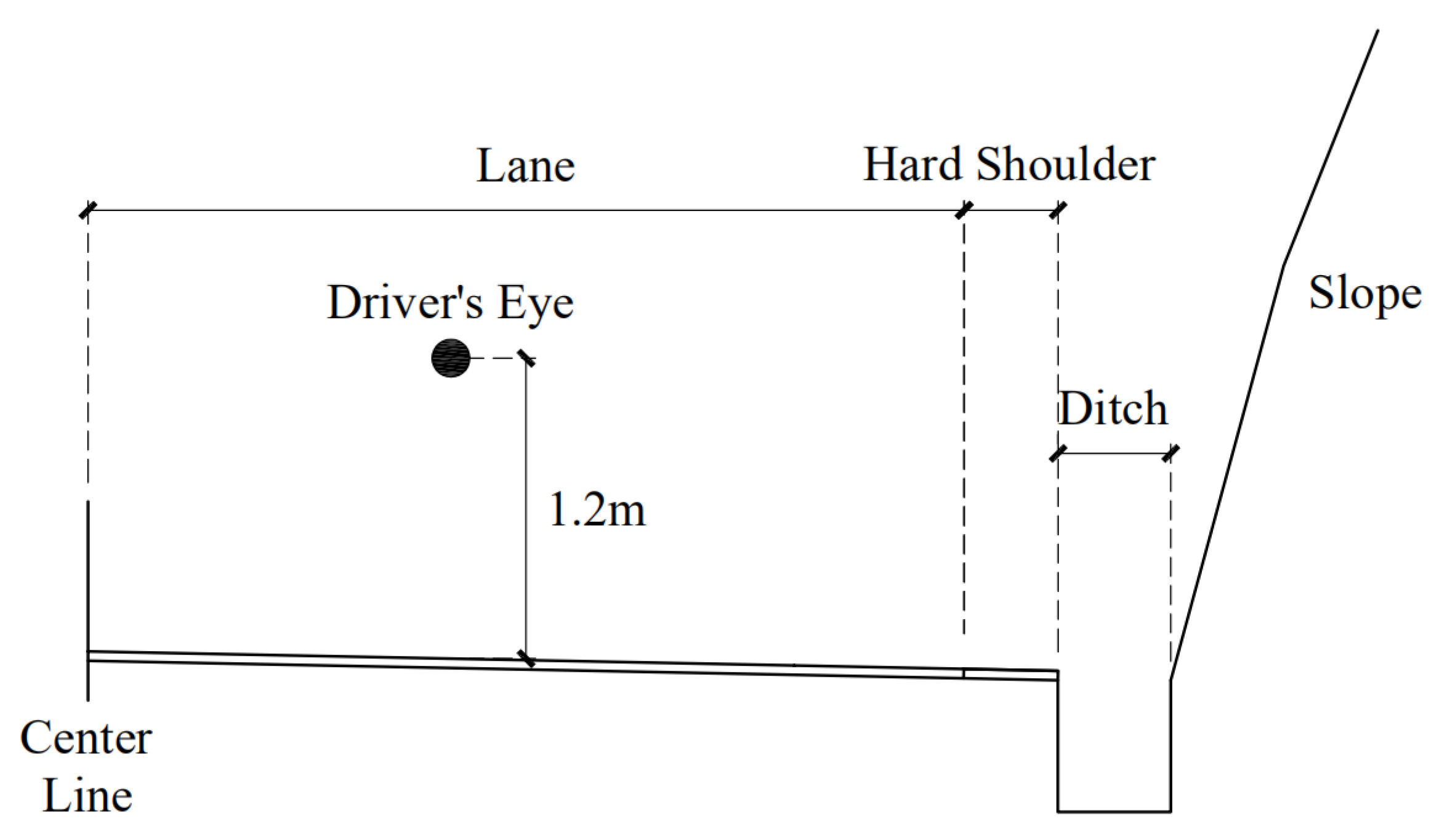
(1)

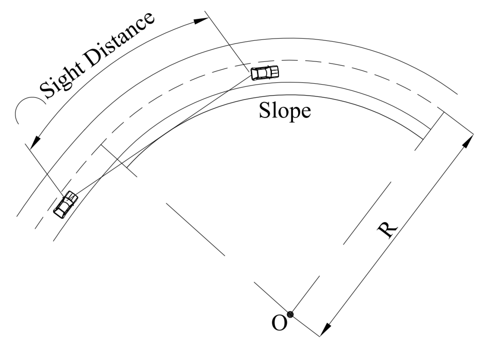
Assume that the car is driving in the center of a lane.

(2)

Assume that the road slope is a curved surface that conforms to the curve of the road.

During the right turn of the basic curve (first transition curve + circular curve + second transition curve), the driver will experience three stages from the first mitigation curve to the circular curve to the second mitigation curve. The unfavorable complexity of the calculation selected in this paper is the sight distance situation when the driver travels to the first transition curve segment and the view is obstructed by the roadside high slope of the circular curve segment, and assumes that the vehicle is traveling in the vertical curve segment at the same time. This is a kind of spatial safety sight distance affected by the overlapping combination of horizontal curve and vertical curve.

3. Calculation of Horizontal S.S.D.

In this paper, based on the horizontal and vertical combination, the three-dimensional sight distance is studied, and the horizontal S.S.D. is calculated by the plane design drawing. It has been assumed that the car is driving in the center of the lane. In AutoCAD (AutoDesk Inc., San Rafael, CA, USA), the road centerline can be shifted the distance of halfway width of the lane to obtain the driving trajectory. In the transition curve section of the curve after the offset, take a point S₀ as the line of sight calculation point, such as Figure 2, where Q is the tangent point between line of sight and slope. Extracting the S₀ coordinates (x₀, y₀) and the center O coordinate (x₀’, y₀’), the S₀O distance can be obtained by the Equation (1):

$$\left|S_{0}O\right|=\sqrt{{\left(x_0^{\prime }-x_0\right)}^2+{\left(y_0^{\prime }-y_0\right)}^2}$$

(1)

Since the driving trajectory line is obtained by shifting the road center line to the inner side of the curve in the above calculation, the actual length of the driving trajectory line is slightly shorter than the length of the road center line. According to Equation (2), the length reduction of the offset curve relative to the original curve can be calculated, so the shortened easement curve length can be obtained.

$${l_s}^{\prime }=l_0-\beta \times D=l_0-l_0^2/\left(2R\times ls\right)\times D$$

(2)

In the formula:

l_s′ is the distance from the SC’ (point of spiral to curve) to the TS’ (point of tangent to spiral) of the curve after shifting inward, the solution here is the full length of the transition curve;

l_s is the length of the original transition curve;

l₀ is the distance from any point on the transition curve of the original road center line to the starting point TS of the transition curve;

β is the transition curve angle;

D is an internal shift value;

R is the radius of the circular curve.

Use the tangent offset method (Figure 3) to calculate the distance from the point S₀ to the offset TS’ point:

$$\{\begin{array}{c}x=l-\frac{l^5}{40R^2{L}_s^2}\\ y=\frac{l^3}{6R{L}_s}-\frac{l^7}{336R^3{L}_s^3}\end{array}$$

(3)

In the formula:

x, y are the coordinates of the points sought;

R is the radius of the curve;

l is the distance from the point of the request to the point TS;

L_s is the length of the transition curve.

However, it is worth noting that Equation (3) is the coordinate system established with TS point of the offset curve as the origin of coordinates and the tangent direction of TS point as the X-axis. Therefore, coordinate system transformation of the coordinate system of S₀ point is required before using this formula. The transformation formula is as follows:

$$\{\begin{array}{c}X=X_{TS}+x\times cosA\pm y\times sinA\\ Y=Y_{TS}+x\times sinA\pm y\times cosA\end{array}$$

(4)

In the formula:

A is the azimuth of the front straight line;

x is X_s0 − X_TS;

y is Y_s0 − Y_TS.

Substituting the coordinates of the converted point S₀ into the Equation (3) can obtain the length from the point S₀ to the point TS’ of the post-offset curve.

Assume that the driver drives to S₀ at this time, and his line of sight is blocked by the high slope at point Q. If the next moment, the driver finds that there is an obstacle at the point D of the line of sight extension (on the driving trajectory). If the driver immediately takes braking measures at this time, the available braking distance is |S₀D|, and |S₀D| is the S.S.D. value on the plane, as shown in Figure 4.

|OQ| = R − d, where d is the distance from the middle line of the road to the slope:

$$d=w+s_b+i\times h$$

(5)

In the formula:

w is the lane width;

S_b is the side ditch and lining size;

i is the slope rate;

h is the height of the slope, that is, the height of the human eye, the small passenger car takes 1.2 m, and the large truck takes 2 m [22].

SC point coordinates are extracted, and the length of line segment between SC and S₀ is calculated by the distance formula. Then Angle S₀OT can be calculated by the cosine formula:

$$\angle S_{0}OT=\arccos \left(\frac{R^2+S_0{O}^2-{\left|SC{S}_0\right|}^2}{2R\times \left|S_{0}O\right|}\right)$$

(6)

So that we can easily calculate the length of |TP|:

$$\left|TP\right|=\left[\arccos \left(\frac{\left|OQ\right|}{\left|S_{0}O\right|}\right)-\angle S_{0}OT\right]\times \left(R-D\right)$$

(7)

In front,$l_s^{\prime }$ and $l_{S_0}$ from S₀ to TS’ after offset are obtained through calculation. S₀:

$$\left|S_{0}T\right|=l_s^{\prime }-l_{S_0}$$

(8)

$$\left|S_{0}P\right|=\left|S_{0}T\right|+\left|TP\right|$$

(9)

|PD| is a section of arc, which can be calculated by the arc length formula:

$$\left|PD\right|=\arccos \left(\frac{\left|OQ\right|}{R-D}\right)\times \left(R-D\right)$$

(10)

Thus, the distance of horizontal S.S.D. |S₀D| is

$$S_h=\left|S_{0}P\right|+\left|PD\right|$$

(11)

4. Calculation of Three-Dimensional S.S.D.

Based on the calculation of horizontal S.S.D., the lengthening effect of the vertical slope on the length of the S.S.D. should be considered, that is to say, the three-dimensional S.S.D. value should be calculated by the combination of horizontal and vertical. Here we need to discuss the situation according to the positional relationship between the highway segment and the vertical curve:

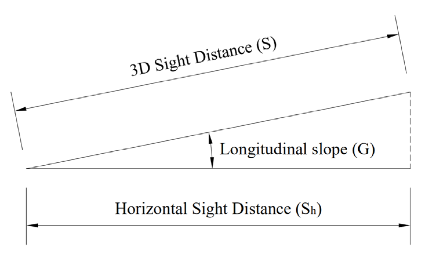
(1)

If the calculation section is a straight slope section (the longitudinal slope value is fixed), the extension effect of the longitudinal slope on the length is linear, as shown in Figure 5. Therefore, the three-dimensional S.S.D. value (Equation (12)) can be obtained by the flat-panel combination calculation.

$$S=S_h\sqrt{1+G^2}$$

(12)

In the formula:

G is the calculation of the longitudinal slope value of the road section.

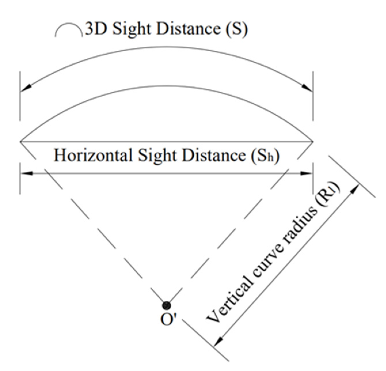
(2)

If the calculation section is in the vertical curve section, the relationship between the three-dimensional S.S.D. and the horizontal S.S.D. is the relationship between the chord and the arc, as shown in Figure 6. Therefore, through the relationship formula of chord length and arc length (Equation (13)), the three-dimensional S.S.D. value (Equation (14)) can be obtained.

$$C=\arcsin \left(L/2r\right)\times 2r$$

(13)

In the formula:

C is the arc length;

L is the chord length;

r is the radius of the arc.

$$S=\arcsin \left(S_h/2R_l\right)\times 2R_l$$

(14)

In the formula:

R_l is the vertical curve radius of the calculated road segment.

The whole calculation process of three-dimensional S.S.D. is summarized into a flow chart, as shown in Figure 7.

5. Instance Verification

5.1. S.S.D. Calculation for a Two-Lane Rural Highway in Guizhou Province

In order to verify the accuracy of the above calculation method, this section will calculate the S.S.D. of the turning section of the actual high road slope. The actual project verified in this paper is a two-lane rural highway in Guizhou province, with a design speed and speed limit of 40 km/h. The roadbed width of general sections is 8.5 m, the width of single lane is 3.5 m, the width of hard shoulder is 0.75 m, the side ditch is rectangular side ditch, the width is 0.6 m, and the lining size of side ditch is 0.25 m (Figure 8). Six curves of PI115 (Point of Intersection, No.115), PI144, PI152, PI317, PI324, and PI369 are selected for 3D S.S.D. calculation. The calculation parameters of each curve are shown in

Table 1. The calculation parameters of S.S.D. calculation.

Intersection	Pile No. at the Center of the Curve	Radius of Circular Curve (m)	Length of Transition Curve (m)	Slope	Vertical Radius (m)
PI115	K173 + 859	60.8	50	1:0.3	2800
PI144	K178 + 841	85.2	35	1:0.3	2800
PI152	K179 + 933	77.5	40	1:0.3	2800
PI317	K217 + 119	97.4	40	1:0.3	-
PI324	K219 + 289	90.0	45	1:0.4	1800
PI369	K229 + 543	102.9	65	1:0.3	-

.

Considering the convenience of calculation, the above calculation methods were programmed in MATLAB (MathWorks Inc., Natic, MA, USA), and the curve parameters were input and calculated, and the results were shown in

Table 2. Calculation results of S.S.D. at each intersection point.

Intersection	PI115	PI144	PI152	PI317	PI324	PI369
Horizontal S.S.D. (m)	46.2241	56.4194	53.0288	57.3197	57.5940	58.3036
3D S.S.D. (m)	46.2246	56.4204	53.0296	57.3483	57.5965	58.4897
Difference (m)	0.0005	0.0010	0.0008	0.0286	0.0025	0.1861

:

From the above calculation results, it is not difficult to find that the difference between horizontal S.S.D. and three-dimensional S.S.D. is not large. However, the difference of the curve on the straight slope section is larger. This is because the radius of the vertical curve is often much larger than the horizontal S.S.D., resulting in a small arc length (three-dimensional S.S.D.) with horizontal S.S.D. as a chord (Figure 6). In contrast, the vertical slope of the straight slope section has a significant effect on the growth of the 3D S.S.D. (Figure 5).

Therefore, when calculating S.S.D. in the vertical curve section, the horizontal S.S.D. can be used instead of the three-dimensional S.S.D., which will greatly reduce the workload of the engineering personnel.

5.2. S.S.D. Inspection Based on Design Speed

Thus, it can be concluded that the S.S.D. at the bend obtained by the above method is 45–60 m, and according to the provisions of “Design specification for highway alignment“ (JTG D20-2017), the minimum value of S.S.D. of passenger car for secondary highways of 40 km/h is 40 m, so the six turns meet the requirements of the design specification.

The method is further verified by the traditional horizontal sightline offset method (Figure 9), which is the distance between the driving trajectory and the line of sight curve. Roadside Design Guide (2011, AASHTO) states that in order to provide sufficient S.S.D., the inside of the flat curve must be guaranteed to have enough H.S.O. (horizontal sightline offset). The H.S.O. required for different radius of the circular curve can be calculated by the S.S.D. with the following Equation (15). If the existing horizontal sightline offset of the project is less than the calculated H.S.O. value, the sight distance does not meet the requirements of the viewing.

$$m=R\left[1-\cos \left(\frac{28.65S}{R}\right)\right]$$

(15)

In the formula:

m is the required horizontal sightline offset (m);

R is the curve radius (m) at the midline of the inner lane;

S is the S.S.D. of the passenger car.

The existing horizontal sightline offset of the road should include the normal distance from the driver’s point of view to the slope of the road. For this project, it includes half lane width, hard shoulder width, side and lining size, slope height, and slope rate. The driver’s viewpoint is considered to be a position shifted to the left by 0.3 m from the center axis of the car. In summary, the current H.S.O. of the project is as follows:

$$m_0=0.3+\frac{3.5}{2}+0.75+0.6+0.25+1.2\times 0.3=4.01m$$

(16)

Substituting m₀ into Equation (15) and R can be calculated. The radius of the right-turning curve needs to reach 59.63 m to meet the safety S.S.D. requirement, and the minimum turning radius in the calculation curve is 60.8 m, so the turn meets the S.S.D. requirements, this is also in line with the calculation results of the calculation method of this paper.

5.3. S.S.D. Inspection Based on Operating Speed

In the process of sight distance verification, the speed is brought into the design speed. In the actual driving process, due to the influence of environment and driver psychology, there is a certain difference between the actual speed of the vehicle and the design speed. We generally use a medium-level driver to define the operating speed based on the actual road conditions, traffic conditions, good weather conditions, etc., and use the 85th percentile speed of the measured speed as the operating speed value.

For the speed measurements we used “Bushnell” brand radar speedometer VELOCITY (10-1911CM type), which has been tested by the Traffic Safety Product Quality Supervision and Inspection Center of the Ministry of Public Security and conforms to the GA297-2001 standard. The device is light in weight, easy to operate, and has high speed measurement efficiency and accuracy. Its technical parameters are shown in

Table 3. Main technical parameters of the speed gun.

Parameters of Our Radar Speedometer	Parameter Values
Speed range	16–320 km/h 10–200 m/h
Detection range	0–390 m
Speed measuring precision	±1.0 mph to ±2.0 kph
Microwave frequency	24.15 Ghz

.

It is worth noting that although the S.S.D. values of the six curves meet the requirements of the design specifications, the author found in the process of speed measurement that there are various degrees of overspeed phenomenon in this section, which will lead to an increase in the time and distance needed by the car in the braking process. The speed test analysis summary is shown in

Table 4. Summary of speed measurement at each intersection (km/h).

Measuring Station	K173 + 000										K180 + 000
Lane	1							2			1			2
Car type	S				M			S		M	M		L	S				M
Speed	37	45	48	42	41	40	31	31	28	30	28	48	31	35	34	30	45	46	37	33
Average velocity	43				37			30		30	38		31	36				39
Operating speed V85	47				41			30		30	37		31	39				42

and

Table 5. Summary of speed measurement at each intersection (km/h).

Measuring Station	K215 + 000														K230 + 500
Lane	1				2										1		2
Car type	S				S					M			L		S		S	M	L
Speed	47	32	28	29	41	36	37	35	35	30	31	44	35	33	31	34	30	35	28
Average velocity	34				37					35			34		33		30	35	28
Operating speed V85	35				38					36			35		34		30	35	28

:

As the speed of the vehicle increases, the sight distance of the vehicle also increases, and the required S.S.D. is also increasing. The 40 m sight distance value in the aforementioned specification is for the design speed of 40 km/h, and when the speed reaches 48 km/h (the maximum speed of small-sized passenger cars measured), the formula in the specification is used to calculate the new required S.S.D.:

$$S_c=\frac{vt}{3.6}+\frac{{\left(v/3.6\right)}^2}{2g\phi }$$

(17)

In the formula:

S_c is small-sized passenger car S.S.D. (m);

v is the operating speed calculation value (km/h);

t is the driver’s reaction time, taking 2.5 s (the judgment time is 1.5 s, the running time is 1.0 s) [22];

g is the acceleration of gravity, taking 9.8 m/s²;

φ is the road surface adhesion coefficient, taken in the wet state, take 0.38.

The calculated S.S.D. with data is 57.2025 m. Therefore, the S.S.D. of PI115, PI144, and PI152 obtained by the calculation method in this paper do not meet the requirements. Then, the result is substituted into Equation (15), and the required minimum circle curve radius is obtained by inverse calculation, which is 85.548 m. Therefore, PI115, PI144, and PI152 calculated by the transverse clear distance method do not meet the requirement, which is consistent with the calculation results in this paper, indicating that the calculation method proposed in this paper is correct and has certain reliability.

6. Conclusions and Future Work

S.S.D. is the key to the safety of braking when the driver encounters obstacles in the process of driving, which is closely related to the safety of national life and property. Therefore, the research on accurate calculation of sight distance is of great significance.

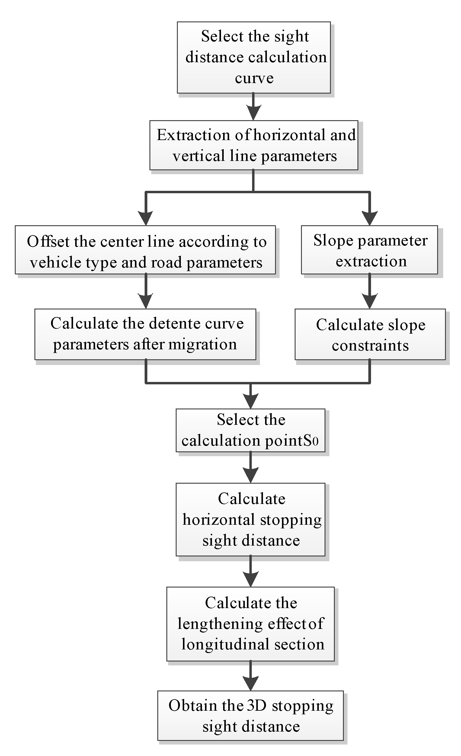
• This article fully considers the actual driving position of the car, the driver’s apparent height, side ditches, and slopes and other actual road driving conditions and establishes a relatively realistic calculation model. Based on the calculation method proposed by highway design parameters, the precise S.S.D. value on the plane is first calculated, and then the height difference between the driver’s viewpoint and the end of the sight line is calculated, and finally the 3D stopping sight distance value is obtained through the principle of horizontal and vertical combination.
• In this paper, the S.S.D. check of actual secondary roads based on the design speed and operating speed is carried out. The results show that the sight distance evaluation result obtained by the calculation method proposed in this paper is consistent with the result of the H.S.O. method.
• The radius of the horizontal curve is the main factor that affects the sight distance of the turning section, while the radius of the vertical curve has a small influence and can be ignored in the actual calculation. That is to say, the plane sight distance can be used to replace the 3D stopping sight distance in vertical curve section.
• Since the calculation method in this paper is sight distance calculation of points, the following research extends point calculation to sight distance calculation of the entire curve through software programming.

References

- Kanellaidis, G.; Vardaki, S. Highway Geometric Design from the Perspective of Recent Safety Developments. J. Transp. Eng. 2011, 137, 841–844. [Google Scholar] [CrossRef]
- Jha, M.K.; Karri, G.A.K.; Kuhn, W. New Three-Dimensional Highway Design Methodology for Sight Distance Measurement. Transp. Res. Rec. J. Transp. Res. Board 2011, 2262, 74–82. [Google Scholar] [CrossRef]
- Castro, M.; Iglesias, L.; Sánchez, J.A.; Ambrosio, L. Sight distance analysis of highways using GIS tools. Transp. Res. Part C Emerg. Technol. 2011, 19, 997–1005. [Google Scholar] [CrossRef]
- Castro, M.; Anta, J.A.; Iglesias, L.; Sánchez, J.A. GIS-Based System for Sight Distance Analysis of Highways. J. Comput. Civ. Eng. 2014, 28. [Google Scholar] [CrossRef]
- Ismail, K.; Sayed, T. New Algorithm for Calculating 3D Available Sight Distance. J. Transp. Eng. 2007, 133, 572–581. [Google Scholar] [CrossRef]
- Hassan, Y.; Sayed, T. Effect of driver and road characteristics on required preview sight distance. Can. J. Civ. Eng. 2002, 29, 276–288. [Google Scholar] [CrossRef]
- Sarhan, M.; Hassan, Y. Three-Dimensional, Probabilistic Highway Design. Transp. Res. Rec. J. Transp. Res. Board 2008, 2060, 10–18. [Google Scholar] [CrossRef]
- Ibrahim, S.E.; Sayed, T.; Ismail, K. Methodology for safety optimization of highway cross-sections for horizontal curves with restricted sight distance. Accid. Anal. Prev. 2012, 49, 476–485. [Google Scholar] [CrossRef] [PubMed]
- Wood, J.S.; Donnell, E.T. Stopping Sight Distance and Horizontal Sight Line Offsets at Horizontal Curves. Transp. Res. Rec. J. Transp. Res. Board 2014, 2436, 43–50. [Google Scholar] [CrossRef]
- Llorca, C.; Moreno, A.T.; Sayed, T.; García, A. Sight Distance Standards Based on Observational Data Risk Evaluation of Passing. Transp. Res. Rec. J. Transp. Res. Board 2014, 2404, 18–26. [Google Scholar] [CrossRef]
- Mavromatis, S.; Mertzanis, F.; Kleioutis, G.; Psarianos, B. Three-dimensional stopping sight distance control on passing lanes of divided highways. Eur. Transp. Res. Rev. 2016, 8. [Google Scholar] [CrossRef][Green Version]
- Wen, H.; Liu, D.; Huang, J. Study on Safe Speed on Nighttime Mountain Highways Based on a Modified Stopping Sight Distance Model. In CICTP 2015; American Society of Civil Engineers: Reston, VA, USA, 2015. [Google Scholar] [CrossRef]
- Gargoum, S.A.; El-Basyouny, K.; Sabbagh, J. Assessing Stopping and Passing Sight Distance on Highways Using Mobile LiDAR Data. J. Comput. Civ. Eng. 2018, 32. [Google Scholar] [CrossRef]
- Moreno, A.T.; Garcia, A.; Llorca, C.; Camacho-Torregrosa, F.J. Influence of highway three-dimensional coordination on drivers’ perception of horizontal curvature and available sight distance. IET Intell. Transp. Syst. 2013, 7, 244–250. [Google Scholar] [CrossRef]
- Moreno, A.T.; Ferrer, V.; Garcia, A. Evaluation of 3d coordination to maximize available stopping sight distance in two-lane rural highways. Balt. J. Road Bridge Eng. 2014, 9, 94–100. [Google Scholar] [CrossRef]
- De Santos-Berbel, C.; Castro, M. Three-Dimensional Virtual Highway Model for Sight-Distance Evaluation of Highway Underpasses. J. Surv. Eng. 2018, 144. [Google Scholar] [CrossRef]
- Osama, A.; Sayed, T.; Easa, S. Framework for evaluating risk of limited sight distance for permitted left-turn movements: Case study. Can. J. Civ. Eng. 2016, 43, 369–377. [Google Scholar] [CrossRef]
- Mampearachchi, W.K.; Masakorala, S.R. Analytical Model for Passing Sight Distance Design Criteria of Two-Lane Roads in Sri Lanka. Transp. Telecommun. 2018, 19, 10–20. [Google Scholar] [CrossRef]
- Chen, Y.-R.; Fu, Y.-T.; Wang, F. Establishment and Application of Sight Distance Computing Model Based on Support Vector Regression. China J. Highw. Transp. 2018, 31, 105–113. (In English) [Google Scholar]
- Zhao, Y.P.; Yang, S.W.; Zhao, Y.F. Analysis of Passing Lane Stopping Sight Distance Outside Median Divider in Expressway. Highway 2004, 10, 39–42. [Google Scholar]
- Wang, X.-N.; Wang, Y.-Z.; Miao, M.-N.; Ou, L. Study and Application of Dynamic Stopping Sight Distance Model. Highway 2015, 60, 151–155. [Google Scholar]
- Design Specification for Highway Alignment, JDG D20-2017. Available online: https://www.chinesestandard.net/PDF/English.aspx/JTGD20-2017 (accessed on 1 May 2020).