Temporal Convolutional Network Connected with an Anti-Arrhythmia Hidden Semi-Markov Model for Heart Sound Segmentation

Featured Application

Combining of temporal convolutional network classifier and improved HSMM model for heart sound segmentation.

Abstract

Heart sound segmentation (HSS) is a critical step in heart sound processing, where it improves the interpretability of heart sound disease classification algorithms. In this study, we aimed to develop a real-time algorithm for HSS by combining the temporal convolutional network (TCN) and the hidden semi-Markov model (HSMM), and improve the performance of HSMM for heart sounds with arrhythmias. We experimented with TCN and determined the best parameters based on spectral features, envelopes, and one-dimensional CNN. However, the TCN results could contradict the natural fixed order of S1-systolic-S2-diastolic of heart sound, and thereby the Viterbi algorithm based on HSMM was connected to correct the order errors. On this basis, we improved the performance of the Viterbi algorithm when detecting heart sounds with cardiac arrhythmias by changing the distribution and weights of the state duration probabilities. The public PhysioNet Computing in Cardiology Challenge 2016 data set was employed to evaluate the performance of the proposed algorithm. The proposed algorithm achieved an F1 score of 97.02%, and this result was comparable with the current state-of-the-art segmentation algorithms. In addition, the proposed enhanced Viterbi algorithm for HSMM corrected 30 out of 30 arrhythmia errors after checking one by one in the dataset.

1. Introduction

Cardiovascular diseases are the main noncommunicable diseases and they contribute to more deaths than all other causes combined [1]. Cardiac auscultation is the most common and cost-effective noninvasive screening method for heart conditions. Despite its universality, auscultation is a difficult technique that requires sufficient experience. Only around 20% of medical interns can effectively perform auscultation [2,3]. Automatic algorithms for auscultation can make the subjective experience of the auscultation technique objective and simplify the mastery of auscultation.

The segmentation of heart sounds is important for improving algorithms for classifying heart sound diseases [4]. One heart sound cycle is generally divided into four states and the states have a fixed order comprising the first sound (S1), systole, the second sound (S2), and diastole, as shown in Figure 1a. S1 is mainly caused by mitral and tricuspid valve closure, and S2 is mainly caused by aortic and pulmonary valve closure. Normally, no sounds appear during systole and diastole, but heart murmurs may appear in systole and diastole to indicate heart diseases, such as valve diseases [5], as shown in Figure 1b.

The two main difficulties that affect heart sound segmentation (HSS) are individual differences and various types of noise. Individual differences such as the frequencies, amplitudes, and durations of heart states may vary according to the physical conditions. The noises introduced in the heart sound signal collection process include breath sounds, ambient noise, and friction sounds caused by shaking. In addition, heart sound signals can be affected by the filtering effects of electronic stethoscopes depending on the filter circuit, material, and shape of the sampling device employed. Thus, the HSS task requires extracting the unique features of S1 and S2 in the heart sound signals, and distinguishing them from various noises.

The previously proposed HSS algorithms were divided into three steps comprising feature extraction, feature classification, and state annotation, and simplified summaries of these methods are shown in

Table 1. Brief summaries of some heart sound segmentation algorithms.

Study	Feature Extraction	Feature Classification	State Annotation
[6]	Shannon energy envelope	Threshold method for peaks	Larger time intervals are the diastolic period; Corresponding time intervals vary more for diastole
[7]	Homomorphic filtering envelope	Peak conditioning process	K-means for time intervals
[8]	Homomorphic envelogram and multiple frequency bands	Duration-dependent hidden Markov model (DHMM)	Viterbi algorithm for DHMM
[9]	Power spectral density functions	Artificial neural network (ANN)	Corresponding time intervals vary more for diastole
[10]	Short-time frequency amplifier and envelope smoothed with a Gaussian smoothing filter	Statistical duration-based assessment methodology	Given directly after S1 and S2 are classified
[11]	Optimized S-transform	Three-nearest neighbor classifier based on singular value decomposition	Given directly after S1 and S2 are classified
[12]	Ensemble empirical mode decomposition (EEMD) combined with kurtosis features	Threshold based on kurtosis features of peaks	Larger time intervals are the diastolic period
[13]	Homomorphic envelope, Hilbert envelope, wavelet envelope, and power spectral density envelope	Logistic regression	Extended Viterbi algorithm
[14]	Mel-frequency cepstral coefficients (MFCCs)	K-means algorithm and ANN	Given directly after S1 and S2 are classified
[15]	Short-time Fourier transform (STFT), homomorphic envelope, Hilbert envelope, wavelet envelope, power spectral density envelope, and MFCCs	Bidirectional recurrent neural networks	-
[3]	Homomorphic envelope, Hilbert envelope, wavelet envelope, and power spectral density envelope	Convolutional neural networks based on U-Net [16]	Sequential max temporal modeling and several different Viterbi algorithms
[17]	Hilbert transform and STFT	Threshold method for peaks	Experience of the amplitudes and remove invalid time intervals
[18]	Homomorphic envelope, Hilbert envelope, wavelet envelope, power spectral density envelope, and MFCCs	Bidirectional long short-term memory with attention	-

. Most algorithms mainly use envelope information and time-frequency information for feature extraction. The envelope and time-frequency features were extracted because the signal amplitudes of S1 and S2 were relatively strong in normal heart sounds, and the frequencies of S1 and S2 mainly fell within a certain range [2]. However, two problems may affect the search for peaks based on the envelopes. First, strong noises may be incorrectly identified as the peaks generated by S1 and S2. Second, S1 and S2 peaks with less sound may be omitted. The positions of S1 and S2 may not be found due to the overlapping of the noise spectrum in the time-frequency based methods.

Therefore, some algorithms aimed to improve the discrimination of S1 and S2 compared with other sounds by modifying the methods for extracting the envelope and frequency features. In order to compare the performance of our algorithm with others, we selected two common features of the four envelopes used in previous studies [3,13,15] and the short-time Fourier transform (STFT) for testing. These four envelopes have been used widely to test the performance of different algorithms, and STFT is a traditional method for spectrum extraction. In addition, we tested a one-dimensional convolutional neural network (1D-CNN) for extracting features by autonomously combining neural networks and compared 1D-CNN with the envelope and spectrum methods.

As shown in Table 1, the most common methods for feature classification included threshold approaches, logistic regression, K-nearest neighbor, recurrent neural networks (RNNs), and CNNs. In previous studies, the algorithms have been used to cluster the time intervals between peaks rather than the features of peaks to distinguish the systole and diastole. The current mainstream algorithms directly classified the features of each time point into heart sound states. Due to the complexity of the actual heart sound signal, in order to improve the classification ability of each time point, the feature extraction step should integrate the signal information for one period or multiple periods of heart sounds, which had a large number of features, so the feature classification algorithm will be complicated. At present, CNN and RNN algorithms are the mainstream algorithms for HSS research. The strong classification capacity of deep learning algorithms is explained by the strong ability of deep neural networks to fit complex functions [19], which is more effective for feature classification with a large number of features. For example, Messner et al. [15] used a bidirectional RNN for classification, which can integrate the long-distance information before and after the classified time point, where the method can obtain excellent direct classification results, but this method was applied to process the whole heart sound signal and the algorithm could only be calculated after acquiring the complete signal. The long short-term memory (LSTM) network is a classical algorithm for RNN and it can allow classification in real time. The classification capacity of LSTM is not as good as that of bidirectional LSTM (BiLSTM), but the difference in performance compared with BiLSTM can be reduced by increasing the cell number, network depth, and error correction methods. Among the CNN methods, Renna et al. [3] used a CNN structure inspired by image segmentation approaches to segment the heart sound states. The results show that when the kernel used by CNN is longer, which means more time points are required to classify the certain time point, the accuracy of the results is higher. The actual times of the kernel used in previous studies were 2.5 s, 5.1 s, and 10.2 s, and the interval between the classified time points was 1/8th of the kernel length. Conventional convolution was employed in the algorithm proposed by Renna et al. [3], so it could only process heart sound signals longer than the kernel length and it could not perform real-time segmentation in the same manner as LSTM. Therefore, we propose using a temporal convolutional network (TCN) to classify the states of the heart sounds, thereby exploiting the advantages of both the RNN and CNN methods, including combining long-distance information with a flexible receptive field size, achieving real-time processing with variable length inputs, parallel computing convolution, and stable gradients in contrast to RNN methods [20].

State annotation involves labeling the entire heart sound signal in a fixed state sequence comprising S1-systole-S2-diastole based on the feature classification results. Some peak-finding algorithms that directly classify the peaks as S1 or S2 can label the signals in a fixed order, whereas other algorithms that do not classify the peaks take the intervals between the peaks as systolic or diastolic based on previous experience that systolic periods are shorter than diastolic periods, or that diastolic periods exhibit more variation. These algorithms based on experience will not make mistakes when classifying normal heart sound signals without noise or other interference, but many actual heart sounds do not match with previous experience. For example, due to illness, some diastolic periods in heart sounds can be shorter than the systolic period, and noise interference can lead to detection errors or the loss of peaks. If certain conditions are not considered, the annotation methods based on the normal heart sound experience will make labeling errors, and thus the application range of these algorithms is limited.

For the current mainstream algorithms based on the classification of each time point by machine learning or the previous classification algorithms based on peak features, it is often not possible to guarantee that the fixed state sequence for heart sounds is correct in the direct classification results, as shown in Figure 2. Direct classification annotation errors are usually caused by irregular noise, but state annotation algorithms can correct their mistakes to satisfy the fixed state sequence rule. One option is to force the output sequence to contain only the admissible transitions among states [3] but this method will be affected by noise and cause shifts in the positions of S1 and S2, because the algorithm is only based on the information from the previous and current two time points. Another algorithm used in previous studies [3,8,13] introduces the state duration probability based on the hidden semi-Markov model (HSMM) model and annotation is conducted with the extended Viterbi algorithm. The extended Viterbi algorithm synthesizes the information in the entire signal for annotation and to the best of our knowledge, it is the best algorithm for heart sound state annotation. However, Messner et al. [15] noted that the extended Viterbi algorithm makes errors when the heart sounds occur with cardiac arrhythmia. In our experiments, arrhythmias occurred rarely in the databases and they had little effect on the final algorithm results, but these errors cannot be ignored in the context of actual disease diagnosis.

According to the previous studies described above, we proposed a framework based on TCN and HSMM for heart sound state segmentation, as well as conducting experiments with the features of STFT, envelopes, and 1D-CNN, and our enhanced Viterbi algorithm ensured that the final state annotation sequence for heart sounds conformed to the fixed order of S1-systole-S2-diastole.

2. Materials and Methods

2.1. Dataset

The electrocardiogram (ECG) is the gold standard for HSS and it is generally considered that the R-peak and end-T-wave of the ECG signal are the corresponding positions of S1 and S2, respectively [13], as shown in Figure 1. Thus, heart sound databases with ECG annotations can be used to verify the performance of the HSS algorithm more realistically than those without ECG annotations.

The public PhysioNet Computing in Cardiology Challenge 2016 has six training sets [21], but only the training-a set (PN-training-a) contributed by the Massachusetts Institute of Technology heart sounds database (MITHSDB) provides complete synchronous ECG recordings, whereas the other five sets lack these data. The original signals for PN-training-a comprise 409 phonocardiogram (PCG) recordings obtained at nine acquisition locations from 121 subjects, where both the PCG and ECG recordings were sampled at 44,100 Hz with 16-bit quantization. In addition to normal PCG recordings, the types of diseases in the heart sound database include mitral valve prolapse, benign murmurs, aortic disease, and other miscellaneous pathological conditions. Due to noise and interference by diseases with ECG in PN-training-a, we manually mark the positions of S1 and S2 based on synchronous ECG recordings. As a result, six recordings were removed due to excessive noise in the ECG or a lack of ECG, and two other recordings were also truncated due to data quality problems. After manual labeling, 403 heart sounds remained, which ranged from 9 s to 37 s, with 117 normal heart sounds and 286 abnormal heart sounds.

MITHSDB is also the source database for the training data used in LS-HSMM (LH-training) [13]. The positions of S1 and S2 marked automatically by ECG algorithms are given directly in the LH-training data set, and these are the standard annotations used most widely in HSS studies. After treatment with LR-HSMM, LH-training contained 792 heart sounds from 135 patients, and the recordings ranging from 1 s to 36 s were down-sampled to 1 kHz. However, according to our experience of labeling based on PN-training-a, ECG algorithms usually cannot avoid all errors and there may be a small number of annotation errors in the LH-training data set, so we conducted experiments using PN-training-a with our manual labels and LH-training with the annotations given by LR-HSMM.

2.2. Metrics

Similar to Renna et al. [3], we used two metrics in this study. The first metric is the feature classification accuracy, which is the ratio of the correct direct classification results relative to the ground truth state sequence s(t). We used the first metric to compare the performance of the feature classification algorithms. The second metric aimed to detect the S1 and S2 events, as described in previous studies [3,8]. The core event detection concept involved grouping consecutive identical frame labels as one event. The specific parameters used to evaluate the final results comprised the positive predictive value (P₊), sensitivity (Se), and F₁ score. According to Schmidt et al. [8], an event is a true positive (T_p) when the center time point of an S1 or S2 event in the calculated sequence ŝ(t) was within 60 ms of the center time point of the corresponding event in the ground truth sequence s(t), whereas all other S1 and S2 events in ŝ(t) were regarded as false positives (F_p). T_total is the total number of S1 and S2 events in s(t), and T_p + F_p is the total number of S1 and S2 events in ŝ(t). Those metrics are calculated as follows.

As shown in Figure 3, in the following, we discussed the three main parts of our algorithm comprising feature extraction, feature classification, and state annotation, as well as focusing on the feature extraction methods, the basic details of TCN, and the annotation methods.

2.3. Feature Extraction

The signal was processed in a uniform manner before feature extraction. The original heart sound recordings were all resampled to 1 kHz and passed through a second-order Butterworth filter within the range from 20–400 Hz.

According to previous studies [3,13,15], we employed the homomorphic envelope, Hilbert envelope, wavelet envelope, and power spectral density envelope as the envelope features. Four envelopes were extracted from the filtered signal and downsampled to 50 Hz, and thus one time point in the feature sequence contained more than 20 ms of information from the original heart sound signal. Finally, all of the envelopes were normalized to zero mean and unit variance.

We applied STFT in order to extract the frequency information for the signal, as described by Messner et al. [15]. We also used a Hamming window with a window size of 80 ms and 75% overlap, so the feature sampling rate was also 50 Hz. Compared with the durations of the states in heart sounds, which were generally more than 60 ms, the frequency of features is 50 Hz, which could reduce the calculations required and ensured that the boundaries of different heart sound states were relatively clear.

The two feature extraction methods described above were based on traditional signal processing methods. Due to the development of deep neural networks, it was possible to design neural network architectures that allowed the network to autonomously learn the features from the original signals. We also used 1D-CNN to directly process the original heart sound signals, thereby allowing the network to directly learn the feature extraction method.

If the original signals in the heart sounds were x(t), where for t = 0, …, T−1, and t indicates the time instants of signal acquisition, and the fragment of the original signal to be convolved is X_n(i) = [x(n·τ) ⋯ x(n·τ+i)] for n = 0, …, N−1, i = 0, …, M−1, where τ is the stride size, n indicates all the time points for features, and M is the kernel length of 1D-CNN. One filter of 1D-CNN is f = [W₀ ⋯ W_i] for i = 0, …, M−1, then the formula used for calculating 1D-CNN is as follows,

$${\mathit{Z}}_{\mathit{f}}\left(n\right)={\mathit{X}}_{\mathit{n}}\ast \mathit{f}={\displaystyle \sum }_{i=0}^{M-1}x\left(n·\tau +i\right)·W_i$$

(1)

This formula yielded a sequence Z_f(n) for n = 0, …, N−1, which could be considered the primary extraction features produced by 1D-CNN. To ensure consistency with the envelopes and STFT, we set the parameters for 1D-CNN as a kernel size of 80 ms and stride size of 20 ms.

2.4. Feature Classification

TCN is a simple but powerful CNN sequence processing architecture that integrates several CNN techniques [20]. First, as shown in Figure 4, TCN used causal convolution to prevent information leakage from the future into the past, and thus it was necessary to calculate the output for the current time point by only using the features before that time point. Therefore, causal convolution was different from the conventional convolution methods and it could allow real-time processing in a similar manner to LSTM. However, the TCN outputs were only related to the inputs and they were not based on the previous outputs, so TCN differed from LSTM because LSTM was necessary to wait for the predecessor results to obtain the current outputs. Thus, TCN had the advantage of parallel operation.

Second, TCN employed dilated convolution [22], as shown in Figure 5. For a filter f = [W0 ⋯ Wi] for i = 0, …, M−1 and the complete input feature sequence Z(t), the formula for the dilated convolution operation F is as follows [20],

$$\mathit{F}\left(s\right)=\left(\mathit{Z}{\ast }_d\mathit{f}\right)\left(s\right)={\displaystyle \sum }_{i=0}^{M-1}\mathit{f}\left(i\right)·{\mathit{Z}}_{s-d·i}$$

(2)

where d is the dilation factor, M is the filter size, and s−d·i denotes the positions of the features that need to be calculated in the past. d determines the number of interval time points between every two adjacent filter taps. When d = 1, a dilated convolution became a conventional convolution. The receptive field could be expanded rapidly by increasing the factor d for dilated convolution in a layer by layer manner. The receptive field could be roughly understood as the length needed for the input features for each output. In general, compared with conventional CNN, TCN using dilated convolution greatly reduced the amount of calculations required when the receptive field is the same size.

Third, each TCN layer used residual connections [23], which were calculated with the following formula,

$$O=Activation\left(x+\mathit{F}\left(x\right)\right)$$

(3)

The residual structure allowed the results from each layer to be merged into the final layer, and thus each layer could be effectively learned. The extensive use of residual structures in deep learning also demonstrated the benefit of this structure. TCN employed a generic residual module instead of a convolutional layer to improve the stabilization of the deep network, as shown in Figure 6.

In addition, as shown in Figure 7, TCN could increase the depth of the network by increasing the number of stacks, and thus the receptive field expands rapidly. As mentioned above, the scale of the receptive field could be roughly regarded as the product of the number of residual blocks, kernel size, and the last dilation factor d. RNN could also synthesize long-distance information but it could not accurately control the actual time length of the integrated information in the same manner as TCN [20].

After calculating the features with TCN, we connected a Softmax layer to output four values at each time point as the probabilities of the four states, and the feature classification results were actually the probabilities. In particular, the direct classification results or annotations were obtained according to the state where the corresponding probability was the maximum of the four probabilities at each time point. Thus, direct classification results could determine the classification performance of the feature classification algorithms. In the experimental section, we present comparisons of different classification algorithms.

2.5. State Annotation

As mentioned in the introduction, many errors in the direct classification annotations violate the fixed state order comprising S1-systole-S2-diastole, as shown in Figure 2. If the algorithm can satisfy the natural requirements for the heart sound states, including the fixed order and lasting for a certain time, order errors will be avoided in the final results and the final detection performance for S1 and S2 can be improved, as shown in Figure 8a.

We considered two methods for state annotation. The first method proposed by Renna et al. [3] forced the output sequence to contain only admissible transitions among states based on the direct classification results. The second method was the extended Viterbi algorithm based on HSMM used by Springer et al. [13]. Based on the previous algorithms, we increased the minimum time limit for states with the first method and improved the performance of the extended Viterbi algorithm by changing the weights of the state duration probabilities and the diastolic distribution.

The TCN results comprised the probability values for four states at each time point and the lengths of the TCN results were the same as those of the TCN input feature sequences. For example, the probabilities from one signal were collected in a matrix B, where $0\le B_{t,j}\le 1$ for t = 0, …, N−1, j = 0, 1, 2, 3 and ${\displaystyle \sum }_{j=0}^3{B}_{t,j}=1$. The state annotation algorithm gave the result ŝ(t) according to matrix B, and it should be noted that the length of ŝ(t) is N, which was the length of the feature sequence, rather than T, which was the length of the original heart sound signal. Thus, at the end of the whole algorithm, we used the expand function provided by Springer et al. [13] to expand the annotation result from length N to length T.

2.5.1. Limited Max Sequential Annotation (LMSA)

Define $\tilde{s}\left(t\right)$ as $\tilde{s}\left(t\right)=arg\underset{j}{\max }{B}_{t,j}$, and the formulae given by Renna et al. [3] are as follows,

$$\widehat{s}\left(0\right)=\tilde{s}\left(0\right)$$

(4)

$$\widehat{s}\left(t\right)=\{\begin{array}{c}\tilde{s}\left(t\right),\hspace{1em}\hspace{1em}\hspace{1em}if \tilde{s}\left(t\right)=\left(\widehat{s}\left(t-1\right)+1\right) mod 4\\ \widehat{s}\left(t-1\right),\hspace{1em}\hspace{1em}\hspace{1em}\hspace{1em}\hspace{1em} otherwise\hfill \end{array}$$

(5)

This method involved a very low amount of calculations but the information combined was only limited to the previous time point, so LMSA was readily affected by noise. According to our previous experience with manual labeling, some algorithm errors were caused by noise that could be avoided by adding a restriction to ensure a set duration time for each state. Heart sounds may exhibit extreme changes of duration for each state but we also require real-time operation, so we added a minimum duration for each state that was uniformly limited to 60 ms. Most S1 and S2 sequences lasted for more than 60 ms [10], and the durations of systole and diastole were longer. When D is the limited duration time, the formula is as follows,

$$\widehat{s}\left(0\right)=\widehat{s}\left(1\right)=\cdots =\widehat{s}\left(D\right)=\tilde{s}\left(D\right)$$

(6)

$$\widehat{s}\left(t\right)=\{\begin{array}{c}\tilde{s}\left(t\right), \begin{array}{c}if \tilde{s}\left(t\right)=\left(\widehat{s}\left(t-1\right)+1\right) mod 4\\ and \widehat{s}\left(t-1\right)=\widehat{s}\left(t-2\right)=\cdots =\widehat{s}\left(t-D\right) when t>D\end{array}\\ \widehat{s}\left(t-1\right), otherwise\hfill \end{array}$$

(7)

However, due to the effects of various types of noise, many errors will still occur with the 60 ms restriction, as shown in Figure 8b. Even after adding the restriction, LMSA depended only on the state information for the previous several time points rather than the complete information for the signal before the time point, so the performance will be highly dependent on the feature classification results. In other restriction methods, some heart sounds did not match with the actual experience that the systolic period was shorter than the diastolic period, so this experience will not be considered. Maximum time limits should also not be imposed for each state because the duration of diastole often varied greatly and adding a very loose restriction was ineffective.

2.5.2. Viterbi Algorithm Based on HSMM

According to Springer et al. [13], HSMM had four main parameters defined as $\lambda =\left(\mathit{A}, \mathit{B}, \mathit{\pi }, \mathit{p}\right)$, where A is the transmission matrix, B is the emission or observation distribution, π is the initial state distribution, and p is the probability of the state duration.

In the HSMM for the HSS task, the four hidden states were S1, systole, S2, and diastole. The output probability matrix obtained from TCN is defined as the matrix B, which is a good approximation based on the experimental results. This kind of estimation can be regarded that the distributions of state and feature are average distribution respectively. The four distributions of the state duration probability used in previous studies [3,8,13] were Gaussian, and all the distribution parameters were rough proportions of one heartbeat time, which was the estimate used in the methods provided by Schmidt et al. [8]. The transmission matrix A and initial state distribution π were invariant, as follows,

$$\mathit{\pi }=\left\{\frac{1}{4},\frac{1}{4},\frac{1}{4},\frac{1}{4}\right\}$$

(8)

$$\mathit{A}=\left[\begin{array}{ccccc}& S1& systole& S2& diastole\\ S1& 0& 1& 0& 0\\ systole& 0& 0& 1& 0\\ S2& 0& 0& 0& 1\\ diastole& 1& 0& 0& 0\end{array}\right]$$

(9)

The HSS task involved obtaining the hidden state sequence for a new heart sound with the known parameter λ for HSMM. Hence, we could use a dynamic programming algorithm to solve this kind of problem, specifically the Viterbi algorithm [13,24]. We defined the length of the entire sequence as N, the number of hidden states as H, the true state at time t as q_t, the entire true states sequence as Q, and the observation sequence as O(t) = [O₁, O₂, ⋯, O_N], where O(t) denoted the features at time point t. Thus, the formula for δ_t(j) [13] is,

$${\delta }_t\left(j\right)=\underset{d}{\max }\left[\underset{i\ne j}{\max }\left[{\delta }_{t-d}\left(i\right)·a_{ij}\right]·p_j\left(d\right)·{\displaystyle \prod }_{s=0}^{d-1}{b}_j\left(O_{t-s}\right)\right]$$

(10)

where δ_t(j) is the likelihood of the most probable state sequence that accounts for the first t observations and ends in state j at time t, and δ₁(j) = π_j b_j (O₁), with 1 ≤ i, j ≤ H, 1 ≤ t ≤ N, 1 ≤ d ≤ d_max, and d_max is set as the duration of a complete heartbeat time.

To find the optimal path for the entire heart sound, the method proposed by Springer et al. [13] found the maximum of δ_t(j) in the range N ≤ t ≤ N + d_max − 1, and decided the hidden state $q_N^{*}$ based on this maximum value when defining $q_t^{*}$ as the hidden state calculated by the algorithm for the final state sequence at the time point t, 1 ≤ t ≤ N. This was the main improvement in the method proposed by Springer et al. [13], and obtaining the extra δ_t(j) was equivalent to the assumption that b_j(O_t) = 1 when N ≤ t ≤ N + d_max - 1 and t ≤ 1.

Next, it was necessary to track back from $q_N^{*}$. The previous transition state for each state was fixed, so the duration time d of the last state $q_N^{*}$ was most important. When calculating the matrix δ_t(j), the method proposed by Springer et al. [13] also recorded the corresponding matrix D_t(j):

$$D_t\left(j\right)=arg\underset{d}{\max }\left[\underset{i\ne j}{\max }\left[{\delta }_{t-d}\left(i\right)·a_{ij}\right]·p_j\left(d\right)·{\displaystyle \prod }_{s=0}^{d-1}{b}_j\left(O_{t-s}\right)\right]$$

(11)

With 1 ≤ i, j ≤ H, 1 ≤ t ≤ N, and 1 ≤ d ≤ d_max. After determining the final state $q_N^{*}$ of the optimal path, the duration time of the final state $d_N^{*}$ was recorded, and thus $q_t^{*}$ when t = N − $d_N^{*}$ + 1,…, N were equal to $q_N^{*}$. The previous state $q_{N-d_N^{*}}^{*}$ could be inferred according to the fixed state transition and $d_N^{*}$. These steps were repeated to obtain all of the annotations for the feature sequence.

In contrast to LMSA, HSMM tracked back the whole signal and integrated all of the information rather than several previous time points, which could avoid changing the state labels when noise occurred, even if the noise appeared suddenly in the middle of a state, and thus the probability of this part being classified as the real state was very low because the time duration of each state tended to be in the high probability range for the Gaussian model, as shown in Figure 9a.

However, Messner et al. [15] showed that the strong anti-noise ability of the HSMM could cause labeling errors when the heart sounds contained arrhythmia, as shown in Figure 10 (TCN + Gauss 1.0). The probability value of a complete optimal path was equal to the classification probabilities at each time point multiplied by the probabilities of each continuous state duration according to the following formula:

$${\delta }_N^{*}\left(q_N^{*}\right)={\displaystyle \prod }_{i=1}^k{p}_{q_i^{**}}\left(d_i^{*}\right)·{\displaystyle \prod }_{j=1}^N{b}_{q_j^{*}}\left(O_j\right)$$

(12)

where k is the total number of continuous state durations in the complete optimal path and $q_{i, 1\le i\le k}^{**}$ denotes the states for each duration. We determined the logarithm on both sides of Equation (12) as open-source code for LR-HSMM and obtain:

$$\log {\delta }_N^{*}\left(q_N^{*}\right)={\displaystyle \sum }_{i=1}^k\log \left(p_{q_i^{**}}\left(d_i^{*}\right)\right)+{\displaystyle \sum }_{j=1}^N\log \left(b_{q_j^{*}}\left(O_j\right)\right)$$

(13)

Which was convenient for computer processing. When the algorithm added an incorrect heartbeat cycle annotation because of arrhythmia, the classification probabilities $\log \left(b_{q_j^{*}}\left(O_j\right)\right)$ became smaller but four state duration probabilities $\log \left(p_{q_i^{**}}\left(d_i^{*}\right)\right)$ are also added instead of one low probability of diastole with an excessively long duration time. Hence, when the algorithm made an error, the increases in the values of the state duration probabilities $\log \left(p_{q_i^{**}}\left(d_i^{*}\right)\right)$ exceeded the decreases in the values of the classification probabilities $\log \left(b_{q_j^{*}}\left(O_j\right)\right)$, thereby resulting in the incorrect optimal path probability becoming higher than the probability of the correct path. In terms of the performance of the whole algorithm, only a few dozen heartbeats with arrhythmia were present in the databases and they had little impact, but arrhythmia is an important indicator of disease, so the algorithm errors caused by arrhythmia could not be ignored.

It has been observed that the diastolic duration usually changes mainly when arrhythmia occurs, and thus the model related to diastole should be considered. First, it is necessary to remove the limit on the diastolic duration because the open-source code for LR-HSMM limits the probability distributions for each state duration to a central range and the probabilities outside the limit range are infinitesimal. However, removing the restrictions was not sufficient to correct the errors. Oliveira et al. [25] noted that using the Poisson distribution instead of the Gaussian distribution can improve the final annotation performance, so we only change the probability distribution for the diastolic duration to the Poisson distribution, as shown in Figure 9b, which can eliminate most of the arrhythmia errors, as shown in Figure 10 (TCN + Poisson 1.0). The Gaussian and Poisson distributions are defined as follows.

• Gaussian distribution:

  $$f\left(x\right)=\frac{1}{\sqrt{2\pi }\sigma }exp\left(-\frac{{\left(x-\mu \right)}^2}{2{\sigma }^2}\right),$$

  (14)
• Poisson distribution

  $$\mathrm{P}\left(X=k\right)=\frac{{\lambda }^k}{k!}{e}^{-\lambda },k=0,1,\dots ,$$

  (15)

Moreover, another method could eliminate the arrhythmia errors. We obtained the logarithm on both sides of Equation (10) using the following formula:

$$\log {\delta }_t\left(j\right)=\underset{d}{\max }\left[\underset{i\ne j}{\max }\left[\log \left({\delta }_{t-d}\left(i\right)\right)+\log \left(a_{ij}\right)\right]+\log \left(p_j\left(d\right)\right)+{{\displaystyle \sum }}_{s=0}^{d-1}\log \left(b_j\left(O_{t-s}\right)\right)\right],$$

(16)

With 1 ≤ i, j ≤ H, 1 ≤ t ≤ N, 1 ≤ d ≤ d_max. As mentioned above, when an arrhythmia error occurred in the optimal path, the impact of the duration probability exceeded the impact of the classification probability, so the weight of $\log \left(p_j\left(d\right)\right)$ could be adjusted to change the influence of the duration probability, and the equation became:

$$\log {\delta }_t\left(j\right)=\underset{d}{\max }\left[\underset{i\ne j}{\max }\left[\log \left({\delta }_{t-d}\left(i\right)\right)+\log \left(a_{ij}\right)\right]+\mathit{\alpha }\log \left(p_j\left(d\right)\right)+{{\displaystyle \sum }}_{s=0}^{d-1}\log \left(b_j\left(O_{t-s}\right)\right)\right],$$

(17)

With 0 ≤ α. When α was reduced to 0.2 from 1, most of the errors caused by arrhythmia could be corrected, as shown in Figure 10 (TCN + Gauss 0.2).

In terms of the complexity and real-time feasibility of the Viterbi algorithm, the main calculation was focused on obtaining the HSMM model parameters and calculating the matrix δ_t(j) based on the feature classification results. The HSMM model parameters that needed to be obtained were mainly related to the heart rate, and the heart rate calculations were based on the autocorrelation with the original signal in the method proposed by Springer et al. [13], which required a large amount of calculations when the signal was excessively long, but the method for determining the heart rate could be simplified by intercepting the signal length or changing the estimation algorithm. Calculating the matrix δ_t(j) required the same amount of calculations at each time point. Thus, after improving the method for estimating the heart rate, the average amount of calculations may not exceed 20,000 at each time point. Thus, compared with the hundreds of thousands of calculations involved in the classification step, the impacts of calculating the heart rate and δ_t(j) were small. In addition, the amount of track-back calculations will be very low and the real-time feasibility will not be affected if the length of the track-back is limited. Therefore, the Viterbi algorithm could also achieve real-time calculations by dynamically refreshing the track-back results.

Other recent improvements to the Viterbi algorithm included searching the sojourn time distribution parameters [26] and a multi-centroid Gaussian model of the diastolic duration [27]. The first improvement employed the expectation maximization algorithm, which was an iterative algorithm that required a large amount of calculations and the calculation time was much longer compared with the original algorithm [3], while it also required long-term signals to achieve better performance, so it was not suitable for real-time segmentation. The second improvement was similar to our algorithm, where it also involved changing the diastolic duration distribution model from a single-peak Gaussian to a multi-peak Gaussian. However, this method also needed long-term signals to find the mean values of the multi-centroid Gaussian distribution, so it is not suitable for real-time operation. In contrast, our improved Viterbi algorithm mainly required the approximate heart rate information that could be obtained within several heartbeat cycles, and it could achieve real-time operation by using a preset heart rate to compensate for the lack of heart rate information in the first heartbeat cycle of the heart sound signal.

3. Results

In the experiments, we used Keras with TensorFlow as a backend to build LSTM and TCN. The feature-length of each signal was padded with zeros to match the length of the longest signal in the two databases and the metrics only included the effective part. After feature classification, we obtained the classification probability matrix B and used the max probability state of each time point to determine the classification state sequence, and we then evaluated its accuracy. We obtained the final state annotation ŝ(t) using the Viterbi algorithm and calculated the F1 score based on the detected events. The activation function used in the TCN networks was ReLU [28], and the activation function employed in the final fully-connected layer was Softmax. Loss of the optimization target was the categorical cross-entropy error, and the optimization method was ADAM [29]. Before training the database, we randomly selected approximately one-quarter of the data as the fixed testing set, and we then trained with the remaining data as the training set by six fold cross-validation, where the training data set was divided into six subjects and trained six times by using a different subject as the validation set every time. We trained each model for 200 epochs and determined the final model parameters according to the validation set with the highest accuracy. Six models were obtained by training the whole data set once, and we applied the six models to the testing set to yield six results, and the final results were produced by averaging the meaningful results.

3.1. Parameter Search for LSTM and TCN

As shown in Figure 11, we tested the features of 80-bin 1D-CNN, 41-bin STFT, 4-bin envelopes, and the 45-bin combination of STFT and envelopes (STFT+envelopes) based on two databases. The cells of one layer shows the results obtained with different numbers of cells in one LSTM layer net and the layers with 200 cells/layer shows the results produced with different numbers of LSTM layers with 200 cells/layer. In order to balance the accuracy and the quantity of the calculations, we decided the parameters for the LSTM network as two layers with 200 cells/layer. In addition, we found that STFT and STFT+envelopes yielded almost the same performance, thereby indicating that envelopes had little effect on increasing the information to STFT. In addition, the hardware implementation scheme for the discrete Fourier transform was sufficiently mature [30], so we employed STFT for comparison in the subsequent experiments, which also enhanced the possibility of a hardware implementation of our algorithm. Moreover, the accuracy of one layer of 1D-CNN was intermediate between that of STFT and envelopes according to the experiments, and the performance of 1D-CNN was significantly weaker than that of STFT.

As shown in Figure 12, we performed parameter search based on the filter numbers and dilation structures for the TCN network, where the kernel size was fixed at two and the stack number was fixed at one. We found that the performance of features was similar to LSTM, so STFT was also selected for comparing the subsequent result. The filter number was selected as 60 and the dilation structure as (1, 2, 4, 8, 16, 32) to ensure that the accuracy and the quantity of the calculations were balanced.

In order to search for the kernel size and stack number, we first fixed the dilation structure as (1, 2, 4, 8, 16, 32) and the number of filters as 60. Figure 13a shows the results obtained with different kernel sizes based on the two databases when the stack number was one, and Figure 13b shows the results with different stack numbers based on the two databases with a kernel size of two. Hence, the other TCN parameters in the subsequent experiments were determined with a kernel size and stack number of two and one, which resulted in the minimum amount of calculations and high performance. Clearly, this type of parameter search approach is incomplete, so we also tried other parameter combinations but the results did not significantly exceed those with our selected values, so the choice of these parameters was sufficiently economic considering the low number of calculations and the requirement for hardware implementation.

Table 2. Comparison of LSTM and TCN.

Net	Accuracy		Parameter Number	FLOPs
	PN-Training-a Testing Set (%)	LH-Training Testing Set (%)
TCN	90.98	92.48	112k	221k
LSTM	91.26	93.13	515k	387k

shows the classification accuracy, parameter numbers, and floating point of operations (FLOPs) for the two LSTM layers with 200 cells/layer and the TCN network with 60 filters, one stack, (1, 2, 4, 8, 16, 32) as the dilation structure and a kernel size of two based on the testing sets. The parameter numbers and FLOPs were obtained using the function provided with TensorFlow. When the performance of TCN was similar to that of LSTM based on LH-training, which is a commonly used data set, the number of parameters and multiply-add calculations were significantly lower with TCN than LSTM.

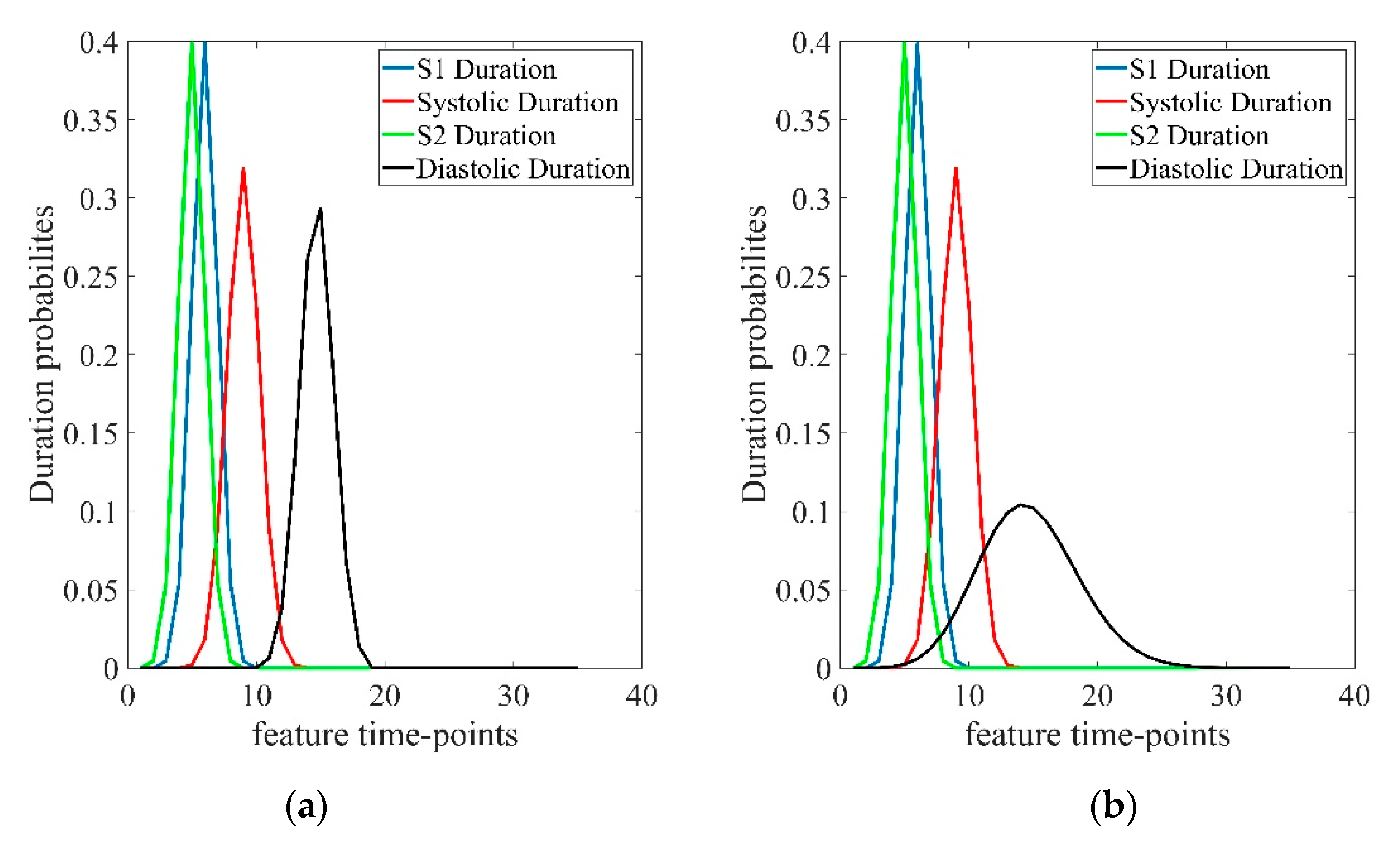
3.2. Fixed State Error Correction

Figure 14 shows the accuracy of the network classification results, as well as the F1 scores detected for S1 and S2 events of different state annotation methods, and it should be noted that the evaluations of the accuracy and F1 scores are different. LSTM and TCN were modeled and tested over 100 times, and a small part of the obvious deviation from the average result was deleted because of over-fitting during network training.

The results shown in Figure 14 indicated that the variability was consistent between the results before and after correction, thereby demonstrating that the accuracy of feature classification greatly influenced the final results. Therefore, it would very useful to identify an algorithm with high accuracy.

The testing results obtained by TCN and LSTM were almost the same with the LH-training testing set, but the error correction results produced by the TCN network with the manually labeled PN-training-a were better than the results yielded by LSTM. Therefore, similar classification results may yield different final results after applying the Viterbi algorithm.

According to the performance of the different error correction algorithms shown in

Table 3. Comparison of various combinations of feature classification methods and state annotation methods using the testing sets in two databases (%).

Combination	Database	Accuracy 1	P+	Se	F1
TCN + LMSA	LH-training	91.86 ± 0.20	96.11 ± 0.25	95.44 ± 0.25	95.77 ± 0.22
	PN-training-a	89.65 ± 0.23	94.81 ± 0.27	92.46 ± 0.3	93.62 ± 0.26
TCN + Viterbi (Gaussian, α = 1)	LH-training	91.23 ± 0.17	96.84 ± 0.19	96.27 ± 0.18	96.56 ± 0.18
	PN-training-a	90.58 ± 0.17	96.08 ± 0.17	94.61 ± 0.18	95.34 ± 0.17
TCN + Viterbi (Gaussian, α = 0.2)	LH-training	91.48 ± 0.18	96.90 ± 0.21	96.75 ± 0.19	96.82 ± 0.19
	PN-training-a	90.58 ± 0.18	96.25 ± 0.18	95.42 ± 0.23	95.83 ± 0.19
TCN + Viterbi (Poisson, α = 1)	LH-training	91.64 ± 0.17	97.25 ± 0.18	96.80 ± 0.17	97.02 ± 0.17
	PN-training-a	90.59 ± 0.17	96.49 ± 0.15	94.99 ± 0.21	95.74 ± 0.17
LSTM + LMSA	LH-training	92.35 ± 0.42	96.61 ± 0.31	95.78 ± 0.38	96.20 ± 0.32
	PN-training-a	89.77 ± 0.74	94.33 ± 0.68	91.96 ± 0.88	93.13 ± 0.76
LSTM + Viterbi (Gaussian, α = 1)	LH-training	91.04 ± 0.29	96.46 ± 0.28	95.90 ± 0.26	96.18 ± 0.27
	PN-training-a	89.08 ± 0.59	94.01 ± 0.69	92.49 ± 0.72	93.25 ± 0.70
LSTM + Viterbi (Gaussian, α = 0.2)	LH-training	91.56 ± 0.31	96.76 ± 0.32	96.67 ± 0.28	96.72 ± 0.30
	PN-training-a	89.54 ± 0.63	94.84 ± 0.65	94.08 ± 0.76	94.46 ± 0.69
LSTM + Viterbi (Poisson, α = 1)	LH-training	91.64 ± 0.31	97.05 ± 0.29	96.75 ± 0.26	96.90 ± 0.27
	PN-training-a	89.50 ± 0.63	95.12 ± 0.62	93.72 ± 0.76	94.41 ± 0.68

¹ Accuracy of the final result after state annotation.

, the results obtained by Viterbi (Poisson, α = 1) and Viterbi (Gaussian, α = 0.2) with TCN and LSTM were similar, and they were significantly better than the results produced with LMSA and Viterbi (Gaussian, α = 1), while Viterbi (Gaussian, α = 1) performed slightly better than LMSA. Based on the similar classification results, the final results showed that TCN performed better than LSTM with PN-training-a. LH-training can be approximately considered as a processed version of PN-training-a, so the results showed that TCN was more stable than LSTM with noise heart sounds. In future mobile applications, the collected heart sounds will be more similar to those in PN-training-a, so TCN is more suitable for future applications on portable devices than LSTM.

Table 4. Comparison of the results of recent several algorithms and TCN + Viterbi (Poisson, α = 1) (%).

Algorithm	Database	Accuracy 1	P+	Se	F1
[13]	LH-training	92.52 ± 1.33	95.92 ± 0.83	95.34 ± 0.88	95.63 ± 0.85
[15]	PN-training-all 2	-	94.9	95.9	95.4
[3]	LH-training	91.7 ± 1.0	95.7 ± 1.0	95.8 ± 1.0	95.7 ± 1.5
[18]	PN-training-all 2	96.9 ± 0.13	96.3 ± 0.42	97.2 ± 0.19	96.70 ± 0.17
LSTM + Viterbi (Poisson, α = 1)	LH-training	91.64 ± 0.17	97.25 ± 0.18	96.80 ± 0.17	97.02 ± 0.17
	PN-training-a	90.59 ± 0.17	96.49 ± 0.15	94.99 ± 0.21	95.74 ± 0.17

¹ Accuracy of the final result after state annotation. ² All training sets of the public PhysioNet Computing in Cardiology Challenge 2016.

compares our best experimental results and the results obtained by several literatures of recent algorithms. It should be noted that many HSS algorithms use different data sets, and the numbers of heart sounds in different databases are all relatively small. Due to the variations in the heart sounds caused by noise interference and heart diseases, the results obtained by various algorithms will differ among databases with variable classification difficulty levels. In addition, the evaluation methods can be different, which will obviously greatly affect the final score, so comparisons of the results should be combined with an evaluation method. The final annotations given in previous studies [3,8,13] and those obtained using TCN + Viterbi (Poisson, α = 1) were corrected with the Viterbi algorithm, so the state labeled all matched with the order of S1-systolic-S2-diastolic, therefore the evaluations were all conducted with event-based approaches. Besides, Messner et al. [15] proposed a new approach based on events for evaluation, but no error correction methods were mentioned, so we speculate that better results can be obtained if error correction is performed after classification. Fernando et al. [18] also reported results obtained without error correction, where the final annotation by the algorithm involved assigning the signal to three states comprising S1, S2, and not S1 or S2, and the evaluation method was the same as the classification accuracy assessment. However, we highly recommend that the Viterbi algorithm is used after feature classification for all HSS tasks, and the evaluation should then be conducted with an approach based on the detection of S1 and S2 events. In general, our algorithm could outperform the current state-of-the-art HSS algorithms, and it had the advantages of real-time processing and the ability to correct most arrhythmia errors.

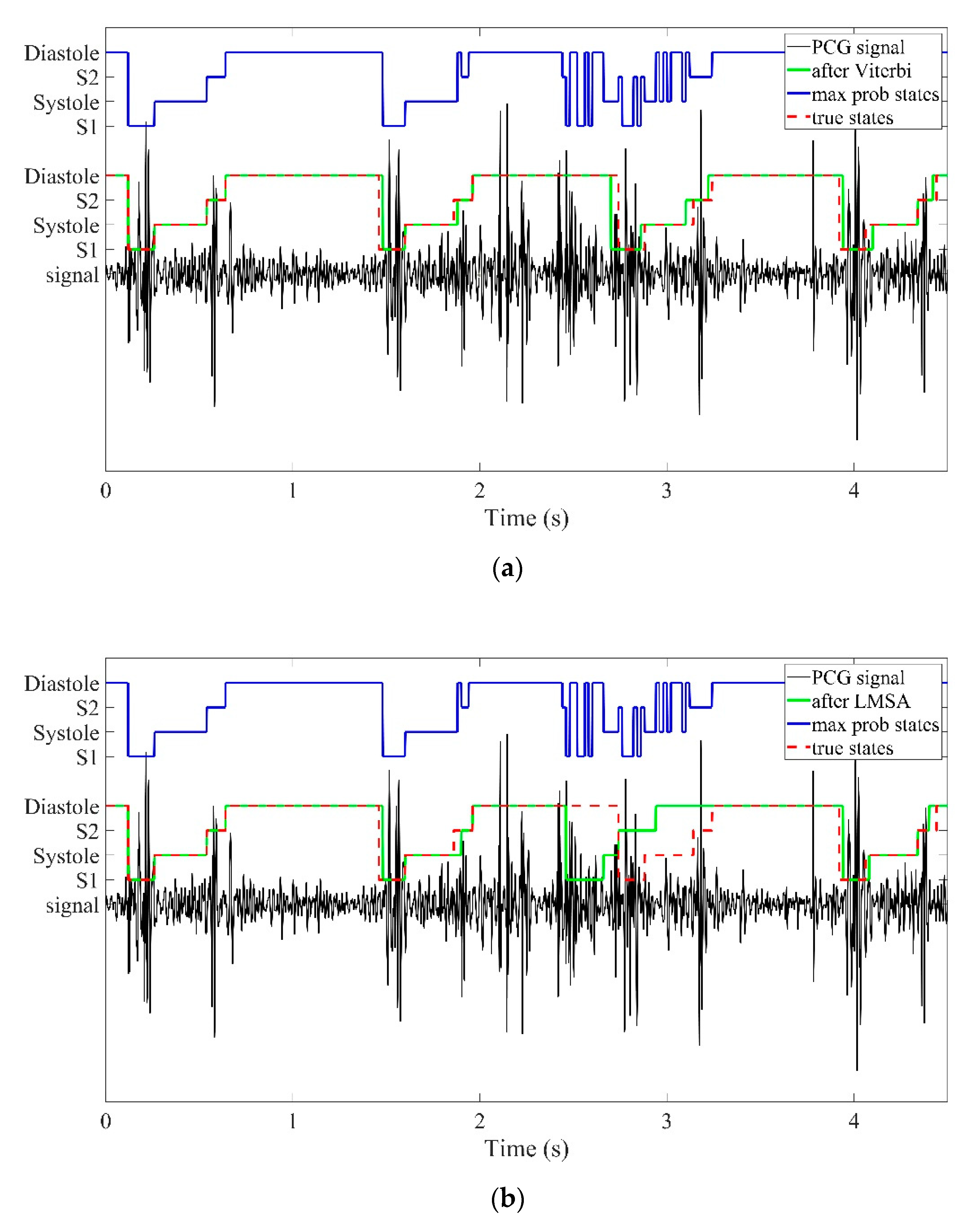
3.3. Arrhythmia Improvement

In order to assess the detection of errors caused by arrhythmia, all of the labels obtained were checked and confirmed. In total, 24 PCG recordings with arrhythmia annotation errors under TCN + Viterbi (Gauss, α = 1) were identified in the two databases. These heart sounds comprised 79 errors due to arrhythmia, with 30 errors in LH-training and 49 errors in PN-training-a, and possibly some of the errors were from the same original recordings. By using TCN + Viterbi (Poisson, α = 1) or TCN + Viterbi (Gauss, α = 0.2), 66 of 79 errors were corrected, with 30/30 errors in LH-training and 36/49 errors in PN-training-a. Two examples are shown in Figure 10. In addition, excessive noise was the main reason for the uncorrectable errors caused by arrhythmia and other problems after applying the state annotation algorithm. These problems need to be solved by collecting more training data, stabilizing the quality of the collection device, improving the quality of the ground truth labels, and other methods.

4. Discussion

The duration distributions of the four states shown in Figure 9b indicate that the Poisson distribution was similar to the Gaussian distribution with a larger variance. After experiments, we found that doubling the variance of the Gaussian distribution in the original algorithm could also correct 66/79 arrhythmia errors, which was inconsistent with the conclusion given by Schmidt et al. [8]. Therefore, due to the development of deep learning and the increased accuracy of classification, the HSS task should involve reducing the influence of the duration probability and optimizing the duration probability model. However, it should be noted that the original Viterbi algorithm (Gaussian, α = 1) can sometimes perform better based on normal heart sounds with severe noise. Thus, continuously improving the algorithms has limitations, so it is equally necessary to reduce the interference due to noise by improving the quality of heart sound collection to support the development of electronic auscultation technology.

As shown in Figure 14, irrespective of the algorithms or databases, the differences between the direct classification results obtained with training sets and testing sets were large, generally because it is considered that the networks are affected by overfitting problems. The occurrence of overfitting can be addressed by using improved network training techniques, such as drop-out and batch normalization. We used some techniques in our experiments, but the effects were small. Therefore, we considered that the possible main reason for overfitting was the lack of available data for training, thereby making the data distributions in the training sets and testing sets inconsistent, especially in those with diseases. Thus, it is necessary to collect more heart sound recordings from many situations for training in order to improve the performance of the feature classification algorithms.

Third heart sound (S3) and fourth heart sound (S4) may appear in diastole due to disease [15]. In terms of the detection of S3 and S4 using the proposed algorithm, the HSMM cannot simply add these two states into hidden states because S3 and S4 are not states of certainty. In order to solve this problem, the algorithm could first assign the signal to S1-systole-S2-diastole, and then perform pattern recognition for S3 and S4 in diastole to detect whether S3 and S4 appear and find their locations. The same method can be used for the diagnosis of heart sound diseases. For example, after performing HSS, the presence of a murmur in systole or diastole can confirm valve problems [31], and whether S2 has a heart sound split indicates pulmonary hypertension [32]. Therefore, detailed annotations are crucial for improving the performance and interpretability of heart sound algorithms. The objectification of heart sound is helpful for doctors to make better diagnoses, thus more doctors can diagnose the patient’s heart sound, which in turn will promote the development of heart sound algorithm.

5. Conclusions

In this study, we proposed an algorithm for segmenting heart sounds using a CNN-based sequence processing architecture, the temporal convolutional networks, which can allow real-time operation with high performance and low computational complexity. We determined the best parameters for TCN by search and compared it with LSTM, as well as testing feature extraction methods using the spectrum, envelopes, and 1D-CNN. In order to correct the heart sound state order errors in the point-by-point classification algorithm, we combined it with the improved Viterbi algorithm. We improved the performance of the Viterbi algorithm by changing the distribution of the diastole and the weights of the state duration probabilities. We conducted experiments with heart sounds from the training database provided by LR-HSMM and the public PhysioNet Computing in Cardiology Challenge 2016 training-set a. We obtained event-based F1 scores of F1 = 97.02% with LH-training and F1 = 95.74% with PN-training-a, which are consistent with the state-of-the-art results. The combination of the algorithm module out of human experience and deep learning network algorithm can be used for other state labeling tasks and as references for other similar studies.

References

1. Shanthi, M. WHO | Global status report on noncommunicable diseases 2014. Women 2015, 47, 2562–2563. [Google Scholar]
2. Chauhan, S.; Wang, P.; Chu, S.L.; Anantharaman, V. A computer-aided MFCC-based HMM system for automatic auscultation. Comput. Biol. Med. 2008, 38, 221–233. [Google Scholar] [CrossRef] [PubMed]
3. Renna, F.; Oliveira, J.H.; Coimbra, M.T. Deep convolutional neural networks for heart sound segmentation. IEEE J. Biomed. Health Inform. 2019, 23, 2435–2445. [Google Scholar] [CrossRef] [PubMed]
4. Clifford, G.D.; Liu, C.; Moody, B.E.; Roig, J.M.; Mark, R.G. Recent advances in heart sound analysis. Physiol. Meas. 2017, 38, E10. [Google Scholar] [CrossRef] [PubMed]
5. Delgado-Trejos, E.; Quiceno-Manrique, A.F.; Godino-Llorente, J.I.; Blanco-Velasco, M.; Castellanos-Dominguez, G. Digital auscultation analysis for heart murmur detection. Ann. Biomed. Eng. 2009, 37, 337–353. [Google Scholar] [CrossRef] [PubMed] [Green Version]
6. Liang, H.; Lukkarinen, S.; Hartimo, I. Heart sound segmentation algorithm based on heart sound envelogram. In Proceedings of the Computers in Cardiology 1997, Lund, Sweden, 7–10 September 1997; pp. 105–108. [Google Scholar]
7. Gupta, C.N.; Palaniappan, R.; Swaminathan, S.; Krishnan, S.M. Neural network classification of homomorphic segmented heart sounds. Appl. Soft Comput. 2007, 7, 286–297. [Google Scholar] [CrossRef]
8. Schmidt, S.E.; Holst-Hansen, C.; Graff, C.; Toft, E.; Struijk, J.J. Segmentation of heart sound recordings by a duration-dependent hidden Markov model. Physiol. Meas. 2010, 31, 513–529. [Google Scholar] [CrossRef] [Green Version]
9. Sepehri, A.A.; Gharehbaghi, A.; Dutoit, T.; Kocharian, A.; Kiani, A. A novel method for pediatric heart sound segmentation without using the ECG. Comput. Methods Programs Biomed. 2010, 99, 43–48. [Google Scholar] [CrossRef]
10. Naseri, H.; Homaeinezhad, M.R. Detection and boundary identification of phonocardiogram sounds using an expert frequency-energy based metric. Ann. Biomed. Eng. 2013, 41, 279–292. [Google Scholar] [CrossRef]
11. Moukadem, A.; Dieterlen, A.; Hueber, N.; Brandt, C. A robust heart sounds segmentation module based on S-transform. Biomed. Signal Process. Control 2013, 8, 273–281. [Google Scholar] [CrossRef] [Green Version]
12. Papadaniil, C.D.; Hadjileontiadis, L.J. Efficient heart sound segmentation and extraction using ensemble empirical mode decomposition and kurtosis features. IEEE J. Biomed. Health Inform. 2014, 18, 1138–1152. [Google Scholar] [CrossRef] [PubMed]
13. Springer, D.B.; Tarassenko, L.; Clifford, G.D. Logistic regression-HSMM-based heart sound segmentation. IEEE Trans. Biomed. Eng. 2016, 63, 822–832. [Google Scholar] [CrossRef] [PubMed]
14. Chen, T.-E.; Yang, S.-I.; Ho, L.-T.; Tsai, K.-H.; Chen, Y.-H.; Chang, Y.-F.; Lai, Y.-H.; Wang, S.-S.; Tsao, Y.; Wu, C.-C. S1 and S2 heart sound recognition using deep neural networks. IEEE Trans. Biomed. Eng. 2017, 64, 372–380. [Google Scholar]
15. Messner, E.; Zohrer, M.; Pernkopf, F. Heart sound segmentation-an event detection approach using deep recurrent neural networks. IEEE Trans. Biomed. Eng. 2018, 65, 1964–1974. [Google Scholar] [CrossRef] [PubMed]
16. Ronneberger, O.; Fischer, P.; Brox, T. U-net: Convolutional networks for biomedical image segmentation. In Proceedings of the International Conference on Medical image computing and computer-assisted intervention, Munich, Germany, 5–9 October 2015; pp. 234–241. [Google Scholar]
17. Thalmayer, A.; Zeising, S.; Fischer, G.; Kirchner, J. A robust and real-time capable envelope-based algorithm for heart sound classification: Validation under different physiological conditions. Sensors 2020, 20, 972. [Google Scholar] [CrossRef] [Green Version]
18. Fernando, T.; Ghaemmaghami, H.; Denman, S.; Sridharan, S.; Hussain, N.; Fookes, C. Heart sound segmentation using bidirectional LSTMs with attention. IEEE J. Biomed. Health Inform. 2020, 24, 1601–1609. [Google Scholar] [CrossRef] [Green Version]
19. Hornik, K. Approximation capabilities of multilayer feedforward networks. Neural Netw. 1991, 4, 251–257. [Google Scholar] [CrossRef]
20. Bai, S.; Kolter, J.Z.; Koltun, V. An empirical evaluation of generic convolutional and recurrent networks for sequence modeling. arXiv 2018, arXiv:1803.01271. [Google Scholar]
21. Liu, C.Y.; Springer, D.; Li, Q.; Moody, B.; Juan, R.A.; Chorro, F.J.; Castells, F.; Roig, J.M.; Silva, I.; Johnson, A.E.W.; et al. An open access database for the evaluation of heart sound algorithms. Physiol. Meas. 2016, 37, 2181–2213. [Google Scholar] [CrossRef]
22. Oord, A.V.D.; Dieleman, S.; Zen, H.; Simonyan, K.; Vinyals, O.; Graves, A.; Kalchbrenner, N.; Senior, A.; Kavukcuoglu, K. WaveNet: A Generative Model for Raw Audio. arXiv 2016, arXiv:1609.03499. [Google Scholar]
23. He, K.; Zhang, X.; Ren, S.; Jian, S. Deep residual learning for image recognition. In Proceedings of the IEEE Conference on Computer Vision & Pattern Recognition, Las Vegas, NV, USA, 27–30 June 2016. [Google Scholar]
24. Yu, S.Z. Hidden semi-Markov models. Artif. Intell. 2010, 174, 215–243. [Google Scholar] [CrossRef] [Green Version]
25. Oliveira, J.; Mantadelis, T.; Renna, F.; Gomes, P.; Coimbra, M. On Modifying the Temporal Modeling of HSMMs for Pediatric Heart Sound Segmentation; IEEE: New York, NY, USA, 2017. [Google Scholar]
26. Oliveira, J.; Renna, F.; Mantadelis, T.; Coimbra, M. Adaptive sojourn time HSMM for heart sound segmentation. IEEE J. Biomed. Health Inform. 2019, 23, 642–649. [Google Scholar] [CrossRef] [PubMed]
27. Kamson, A.P.; Sharma, L.N.; Dandapat, S. Multi-centroid diastolic duration distribution based HSMM for heart sound segmentation. Biomed. Signal Process. Control 2019, 48, 265–272. [Google Scholar] [CrossRef]
28. Glorot, X.; Bordes, A.; Bengio, Y. Deep sparse rectifier neural networks. J. Mach. Learn. Res. 2011, 15, 315–323. [Google Scholar]
29. Kingma, D.P.; Ba, J. Adam: A method for stochastic optimization. arXiv 2014, arXiv:1412.6980. [Google Scholar]
30. Frigo, M.; Johnson, S.G. The design and implementation of FFTW3. Proc. IEEE 2005, 93, 216–231. [Google Scholar] [CrossRef] [Green Version]
31. Ker, J.A. The recognition and management of valvular heart disease. Contin. Med. Educ. 2004, 22, 353. [Google Scholar]
32. Xu, J.; Durand, L.G.; Pibarot, P. A new, simple, and accurate method for non-invasive estimation of pulmonary arterial pressure. Heart 2002, 88, 76–80. [Google Scholar] [CrossRef] [Green Version]
Figure 1. Heart sounds with synchronous electrocardiogram and segmentation results for four states of the heart cycle (S1, systole, S2, and diastole): (a) normal heart sound (b) abnormal heart sound with heart murmur.
Applsci 10 07049 g001
Figure 2. Example of direct classification annotation based on the feature classification results for a noisy heart sound. The feature classification result output from the temporal convolutional network (TCN) comprises the state probabilities for each time point, and the direct classification annotation is the max probability state at each time point.
Applsci 10 07049 g002
Figure 3. Block diagram and visualization of the heart sound segmentation (HSS) algorithm.
Applsci 10 07049 g003
Figure 4. Simplified visualization of causal convolution and conventional convolution.
Applsci 10 07049 g004
Figure 5. Simplified visualization of a TCN with kernel = 2, stack = 1, and dilation structure = [1, 2, 4].
Applsci 10 07049 g005
Figure 6. Residual block.
Applsci 10 07049 g006
Figure 7. Simplified visualization of a TCN with kernel = 2, stack = 2, and dilation structure = [1, 2, 4].
Applsci 10 07049 g007
Figure 8. Examples of state annotation methods for correcting fixed state order errors in the classification result. Max prob states was obtained as the highest probability state for the classification result at each time point. (a) Viterbi algorithm. After Viterbi the state sequence was corrected using the Viterbi algorithm. (b) LSMA. After Limited Max Sequential Annotation (LMSA) the state sequence was corrected by limited max sequential annotation.
Applsci 10 07049 g008
Figure 9. Duration probabilities for four states. The S1, systole, and S2 duration probabilities follow the Gaussian distribution. (a) Gaussian distribution for diastolic duration. (b) Poisson distribution for diastolic duration.
Applsci 10 07049 g009
Figure 10. Comparison of different state annotation algorithms with arrhythmia heart sounds. (a) LH-training No. 555. (b) PN-training-a No. 7. TCN + gauss 1.0 used the previous Viterbi algorithm. TCN + Gauss 0.2 used the Viterbi algorithm changed the weights of the state duration probabilities. TCN + Poisson 1.0 used the Viterbi algorithm changed the diastolic distribution for Poisson distribution.
Applsci 10 07049 g010
Figure 11. Accuracy of long short-term memory (LSTM) classification results. (a) PN-training-a. (b) LH-training.
Applsci 10 07049 g011
Figure 12. Visualization of the accuracy of TCN with different filter numbers and dilation structures. (a) PN-training-a. (b) LH-training. The ordinate denotes the different number of filters and abscissa represents the dilation structure. For example, abscissa number 16 indicates that the dilation structure is (1, 2, 4, 8, 16), and the meanings of other abscissa numbers are similar.
Applsci 10 07049 g012
Figure 13. Accuracy of TCN classification results with different kernel sizes and stack numbers. (a) kernel. (b) stack.
Applsci 10 07049 g013
Figure 14. Comparison of results obtained before and after different state annotation methods. (a) PN-training-a. (b) LH-training.
Applsci 10 07049 g014