Numerical Study for the Effects of Temperature Dependent Viscosity Flow of Non-Newtonian Fluid with Double Stratification

 ,
,  and
and 
Abstract
1. Introduction
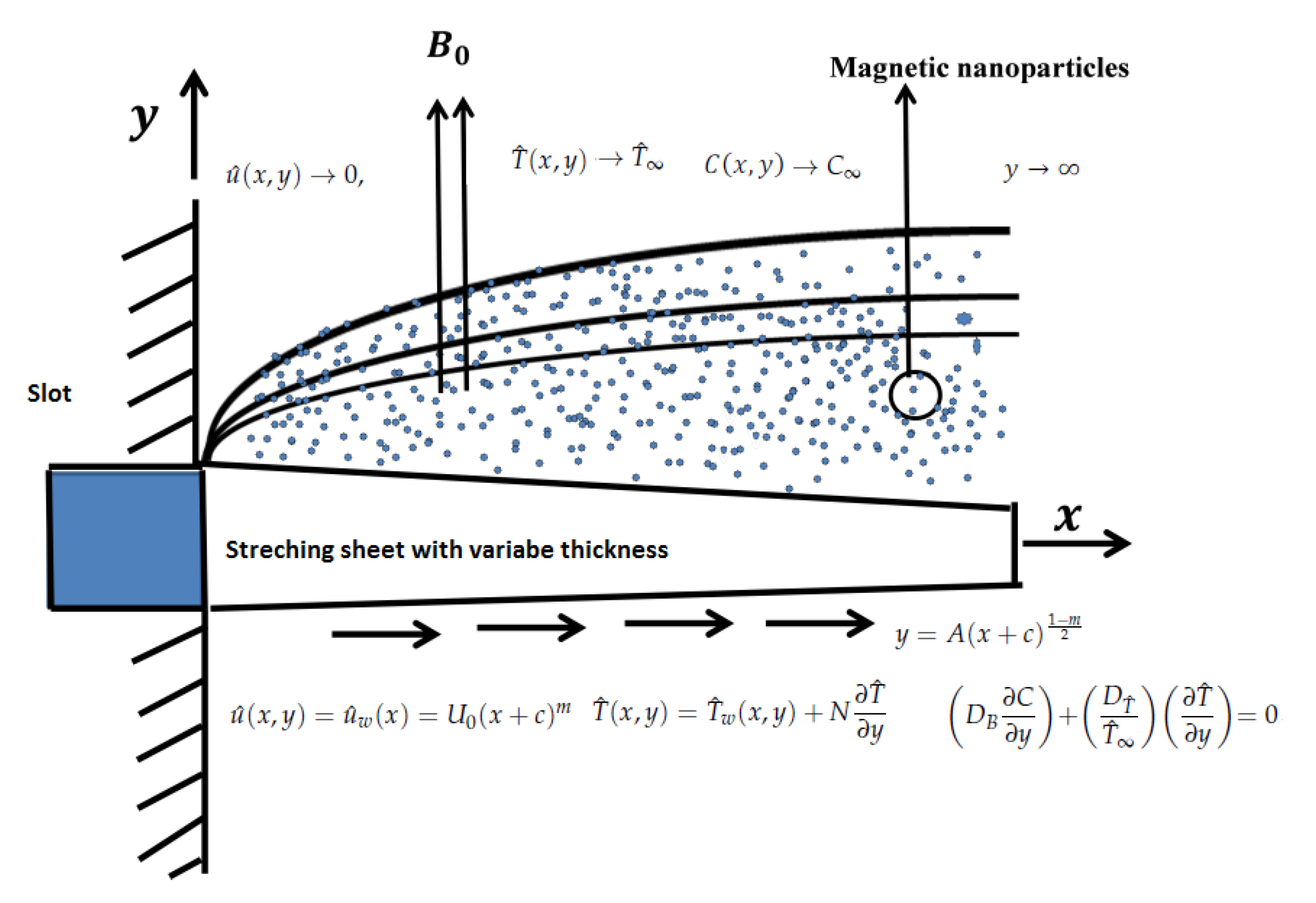
2. Mathematical Model
3. Numerical Method
4. Results and Discussions
5. Conclusions
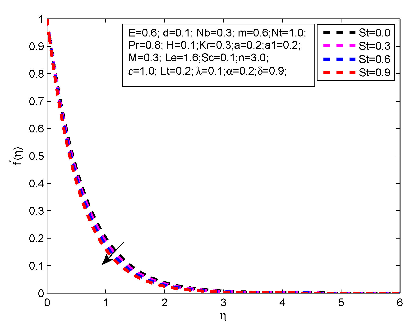
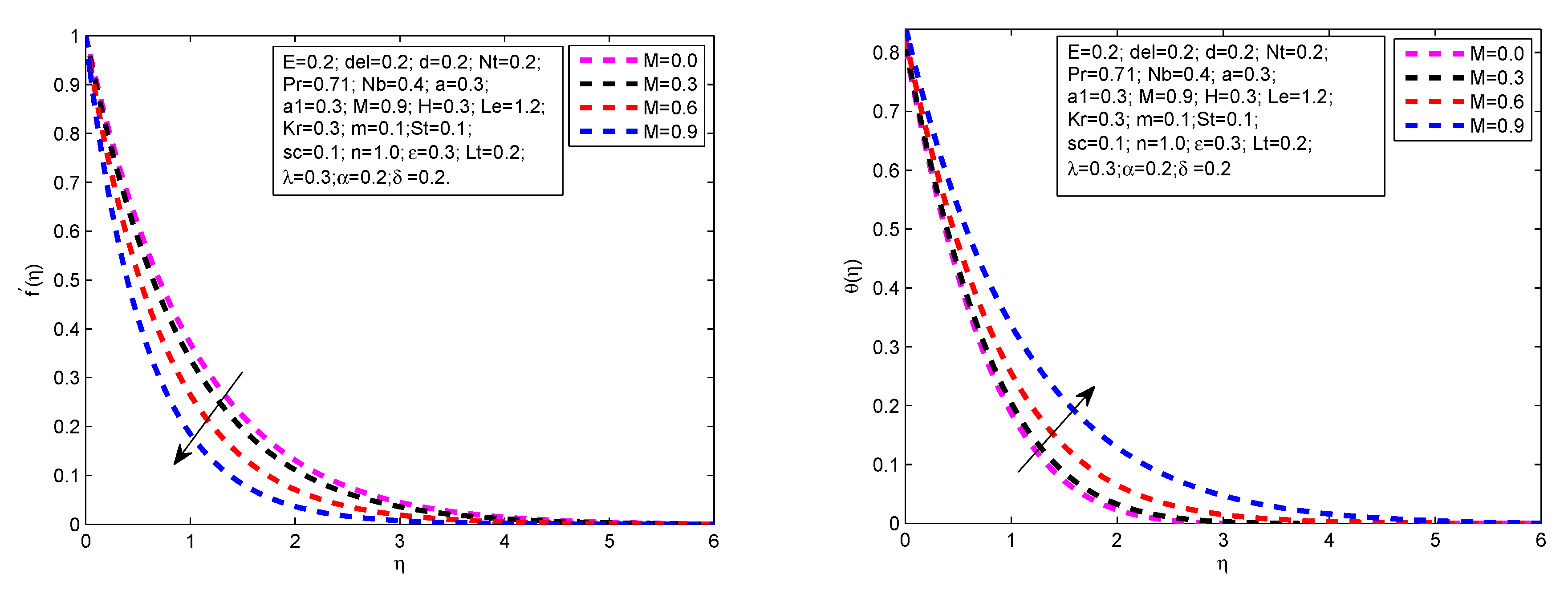
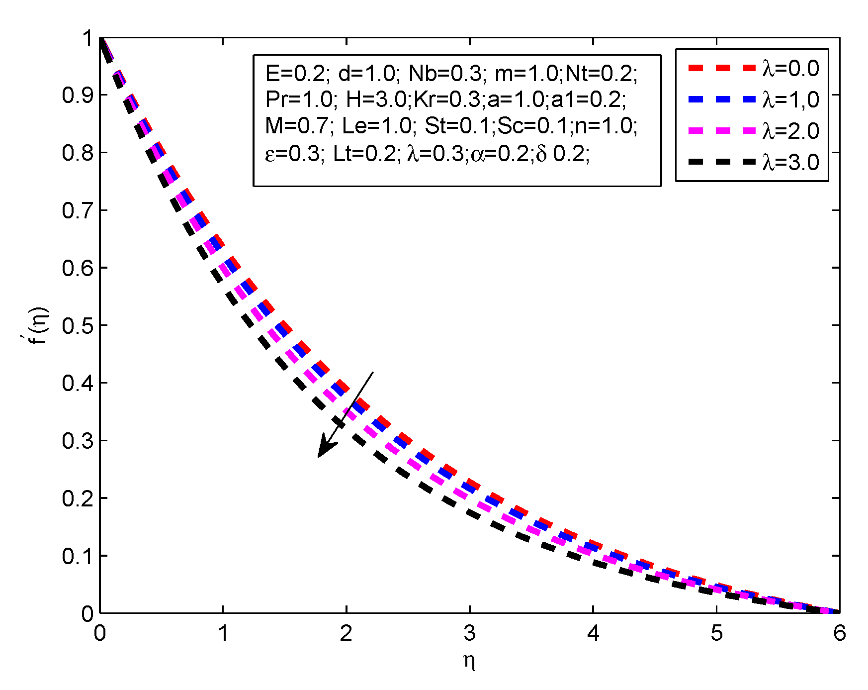
- There is a decreases in velocity profile with increasing values of , m, and M
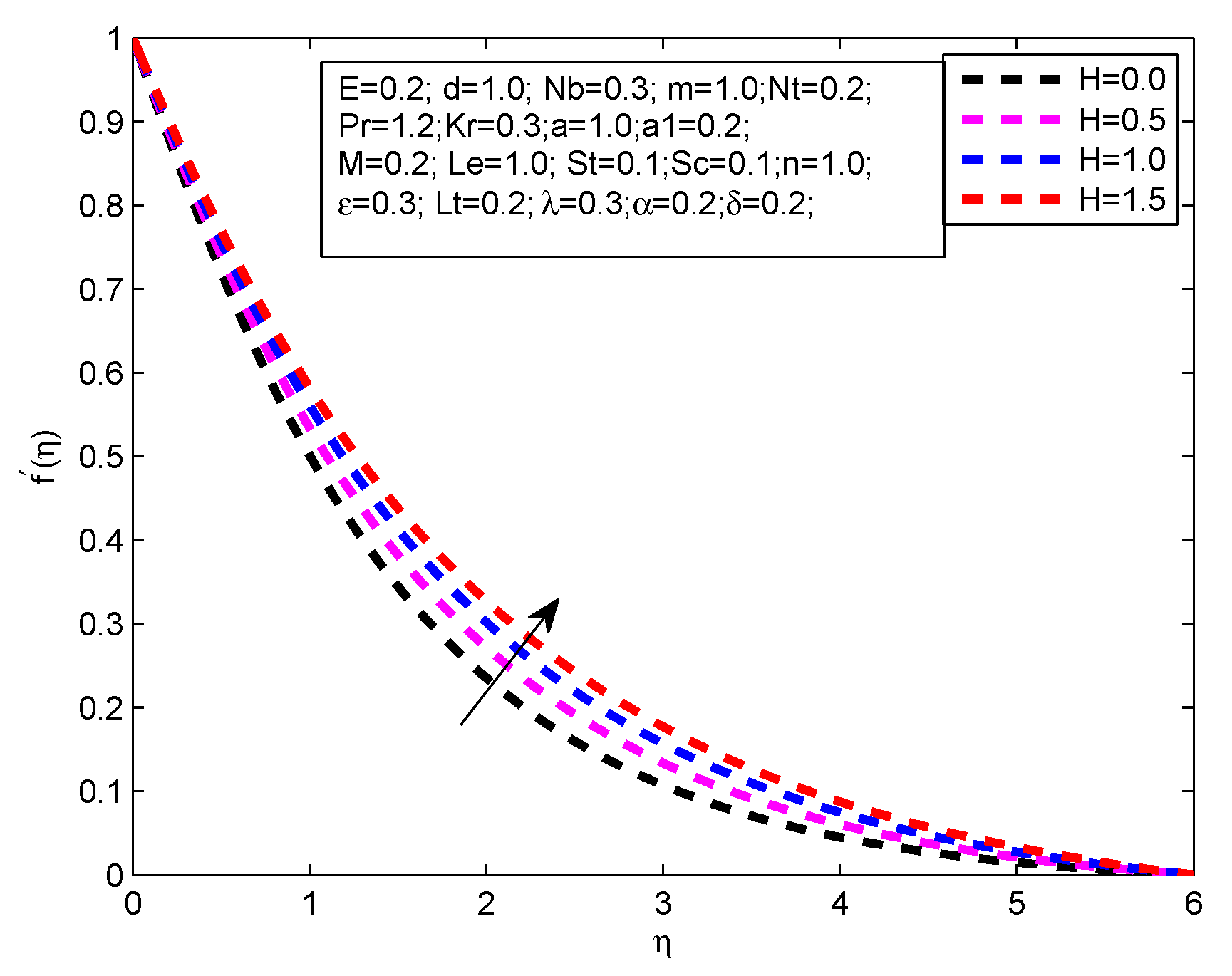
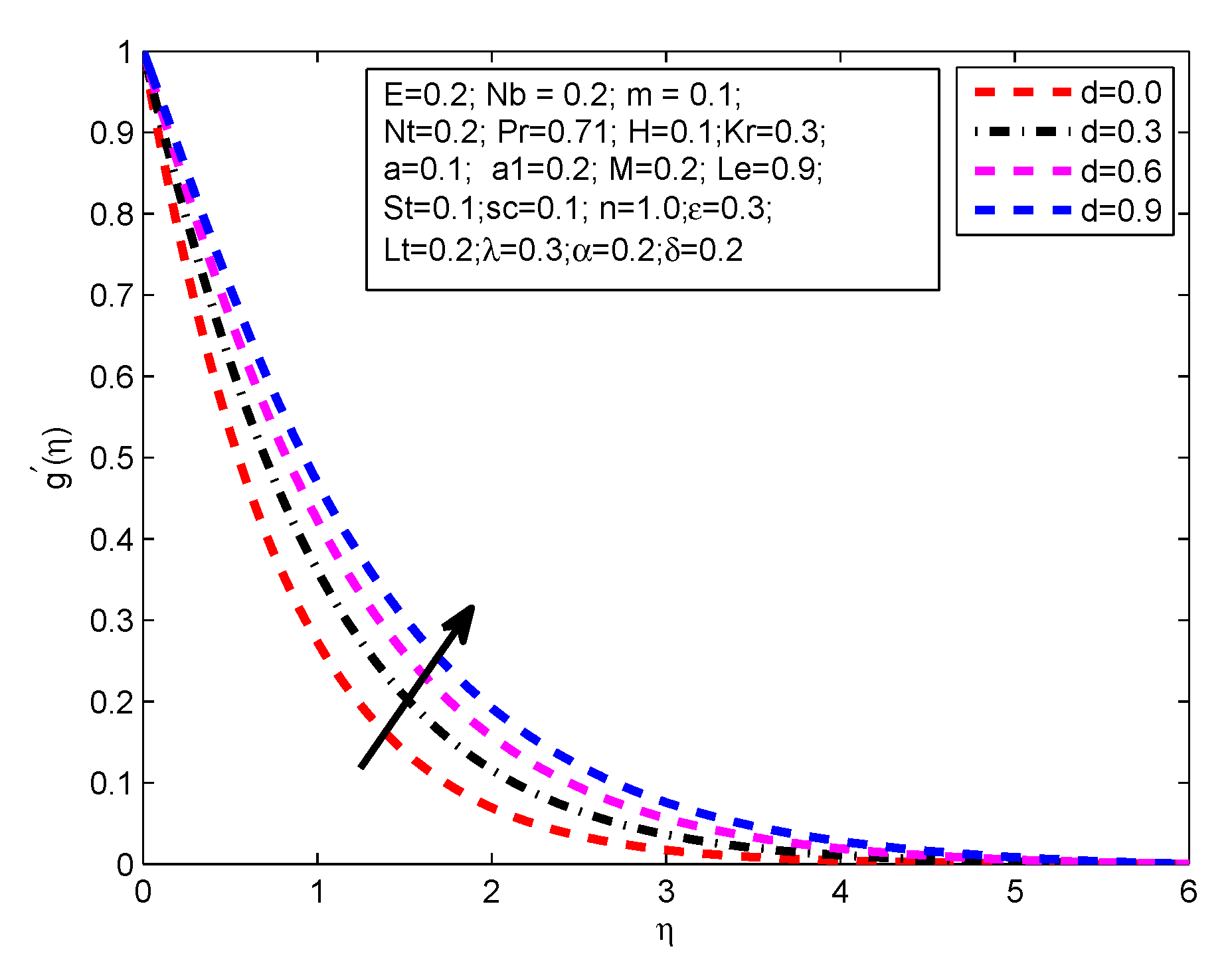
- There is a increases in velocity profile with increasing values of H and .
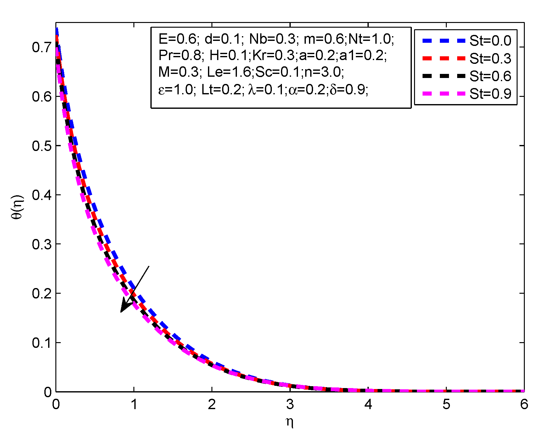
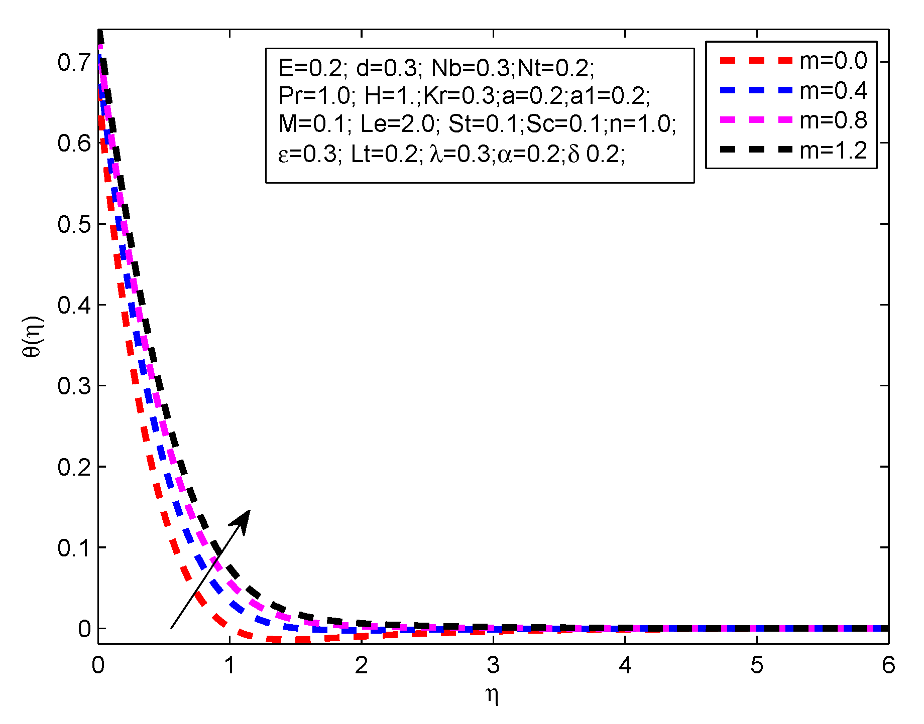
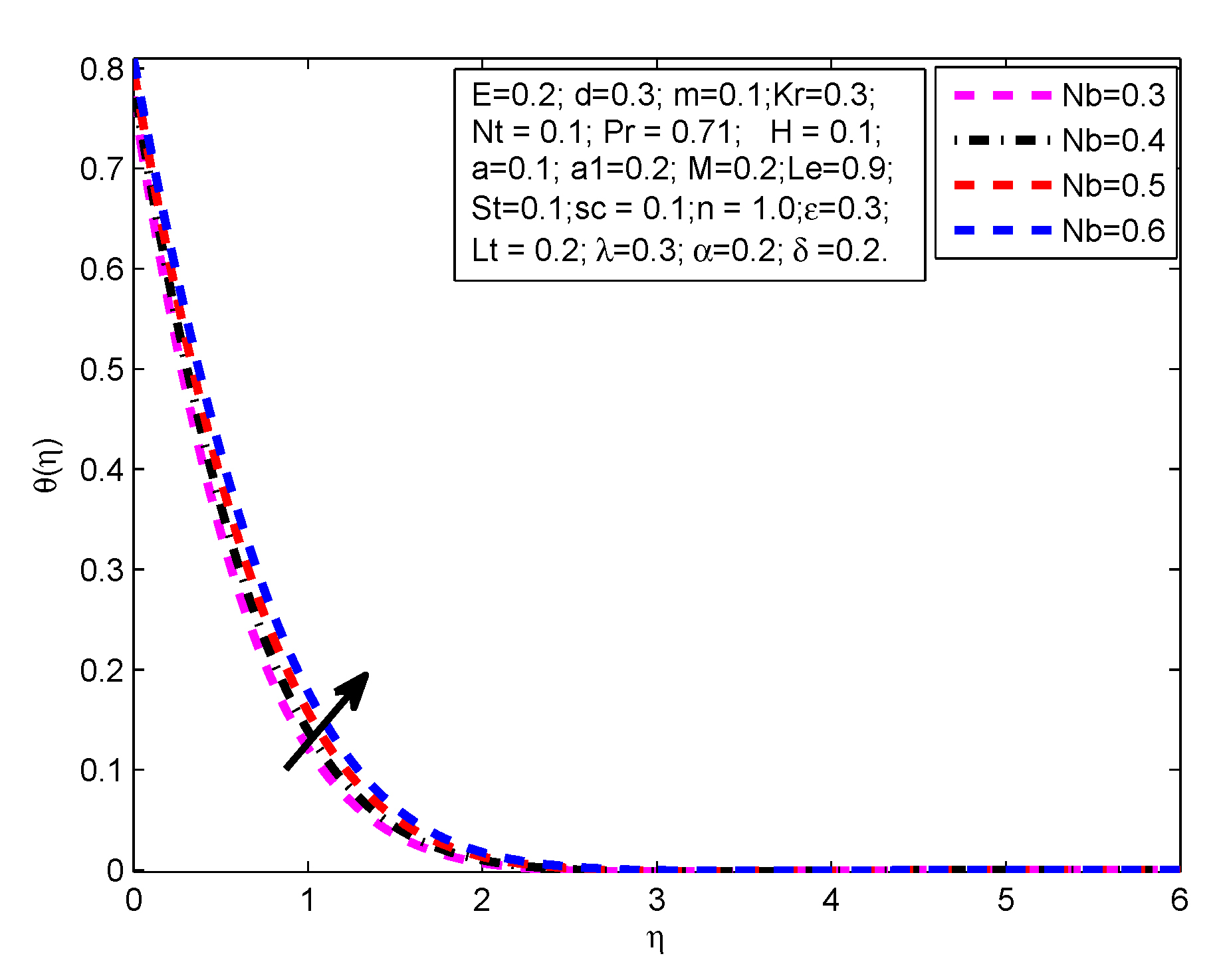
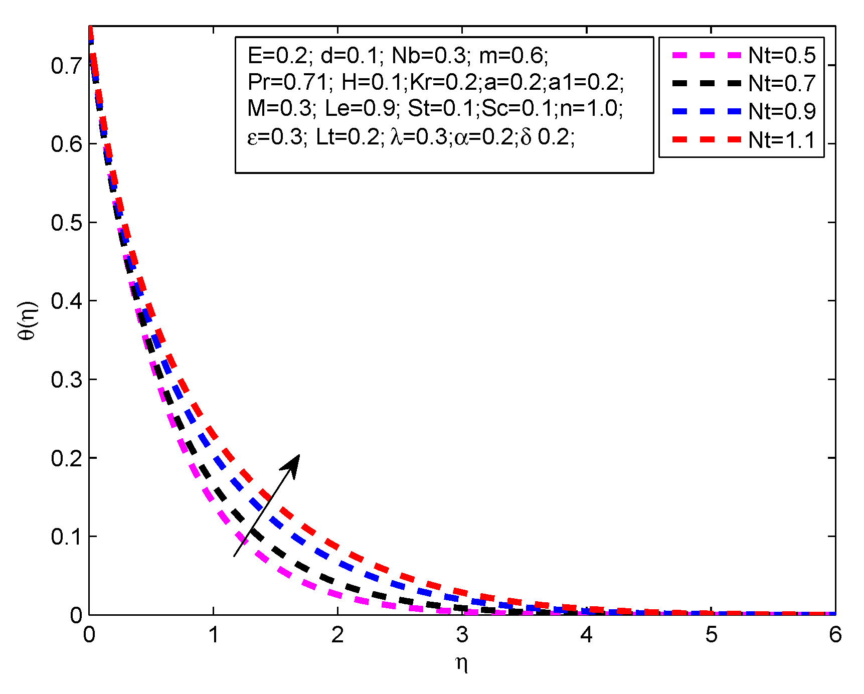
- The temperature profile increases with the exceeding values of M, R, m, H, L, and .
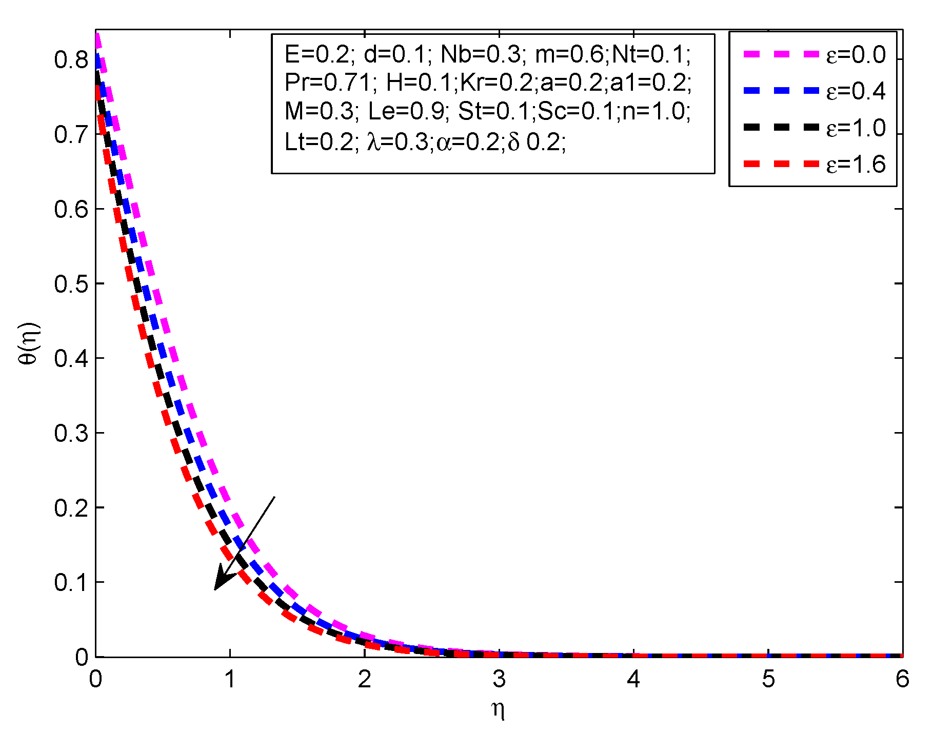
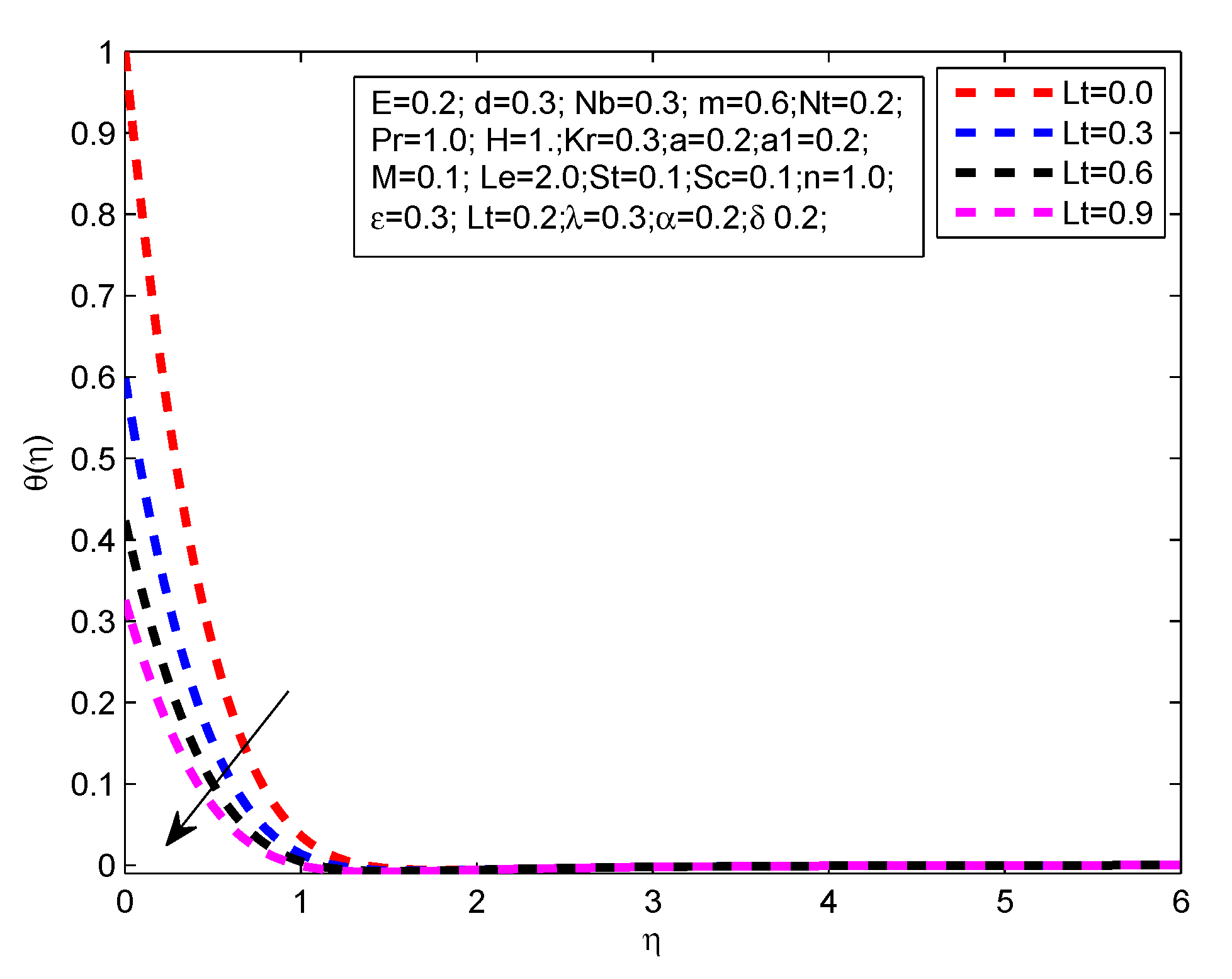
- Decrease in temperature profile is noticed for the increasing values of , , , n and M.
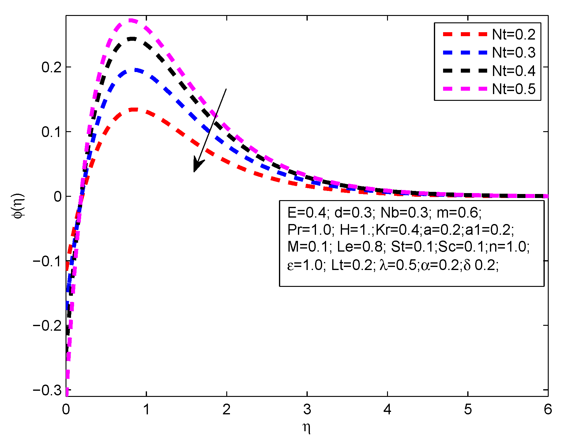
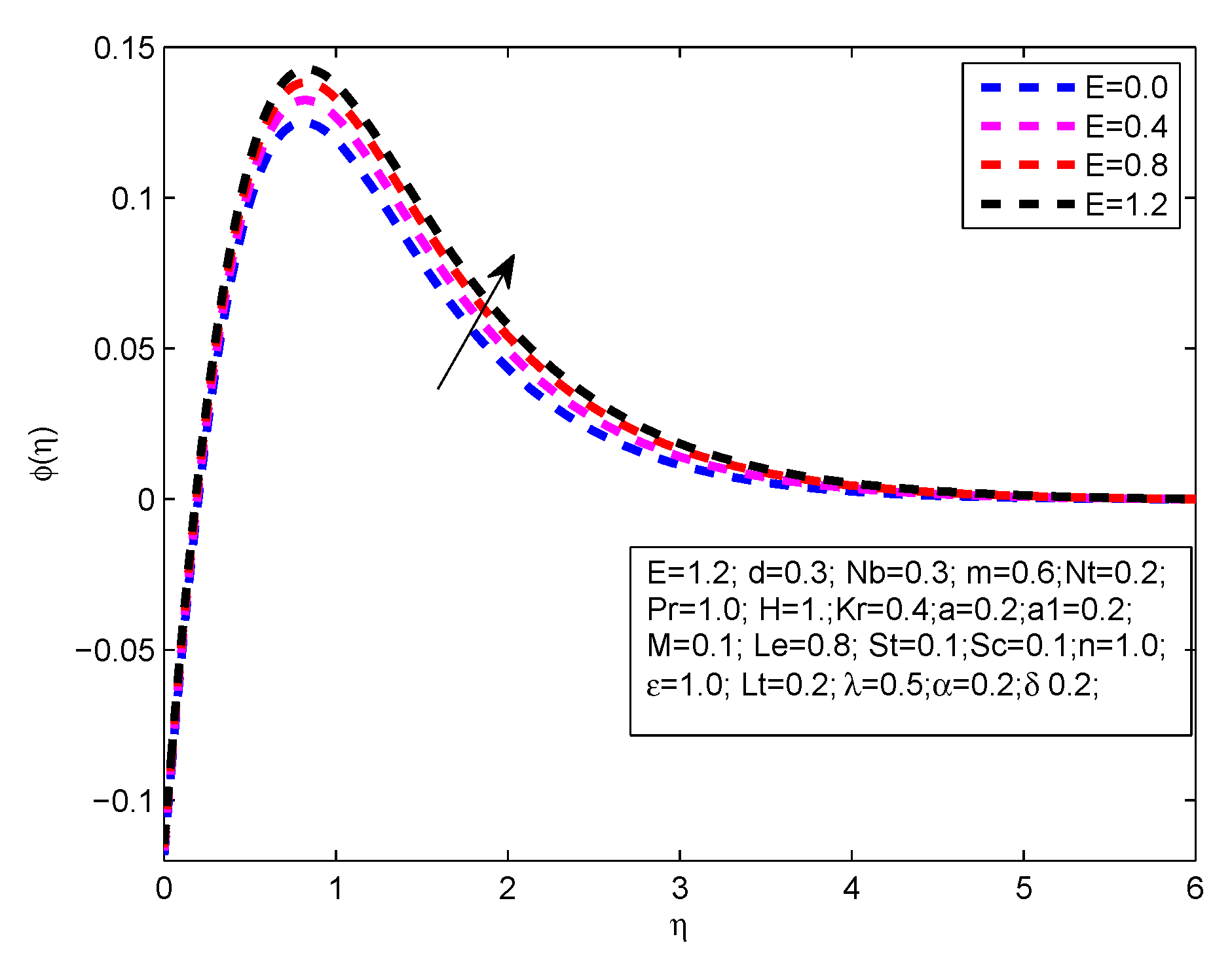
- The concentration profile increments for large values of M, E and H.
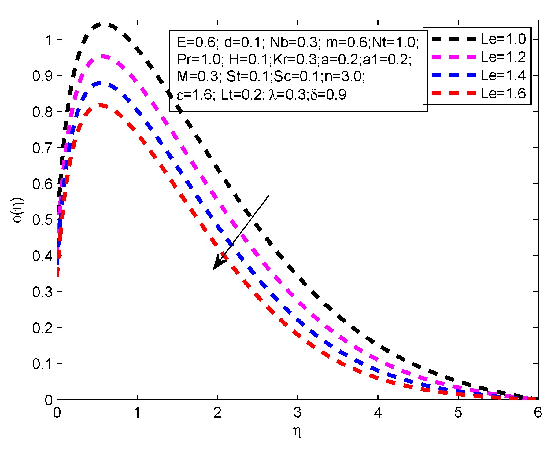
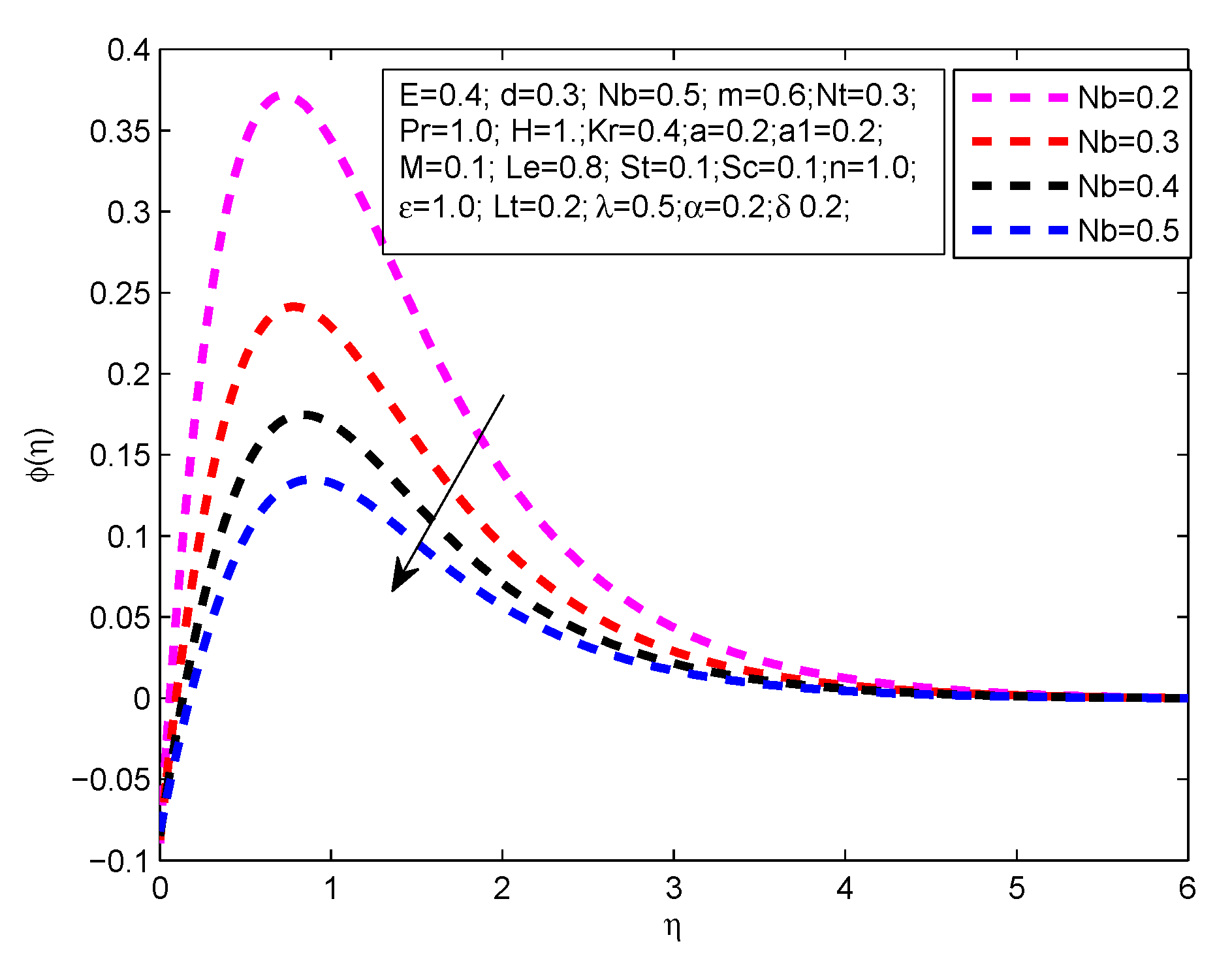
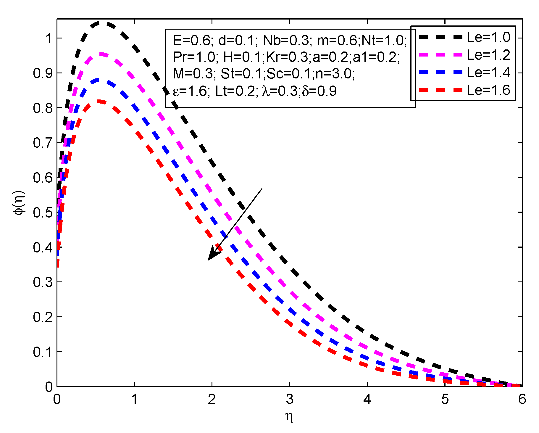
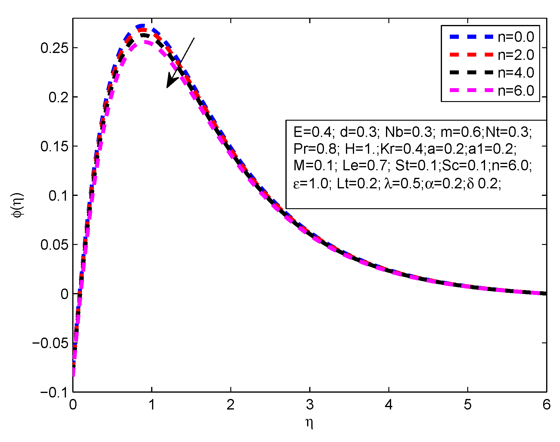
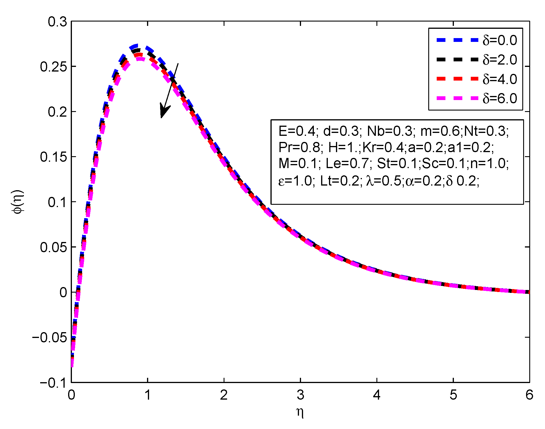
- The concentration profile reduces with the steps up values of , , n, and .
Author Contributions
Funding
Conflicts of Interest
Abbreviations
| Ordinary Differential Equation | Magnatohydrodynomics | ||
| Boundary value problem | Thermal conductivity | ||
| Initial value problem | Free stream conductivity | ||
| m | Velocity power index parameter | Reaction rate parameter | |
| Wall thickness parameter | Temperature dependent viscosity parameter | ||
| E | Activation energy | n | Fitted rate constants |
| Local skin friction | Fluid parameters | ||
| Specific heat | Temperature relative parameter | ||
| g | Dimensionless velocity | stratification parameters | |
| Local wall couple stress | Brownian motion parameter | ||
| Local Nusselt number | Thermophoresis parameter | ||
| Prandtl number | Lewis number | ||
| Reaction rate parameter | Thermal Slip parameter | ||
| Wall heat flux | M | Magnetic parameter | |
| Sherwood number | Plate surface | ||
| Reynolds number | Variable thermal conductivity | ||
| Thermo-phoretic parameter | d | Temperature dependent viscosity parameter | |
| Ambient temperature | Wall temperature | ||
| u | Velocity component in x–direction | v | Velocity component in y –direction |
| Viscosity | Magnetic induction | ||
| Boltzmann constant |
References
- Sakiadis, B. Boundary-Layer Behavior on Continuous Solid Surfaces: II. The Boundary Layer on a Continuous Flat Surface. AIChE J. 1961, 7, 221–225. [Google Scholar] [CrossRef]
- Vleggaar, J. Laminar boundary-layer behaviour on continuous, accelerating surfaces. Chem. Eng. Sci. 1977, 32, 1517–1525. [Google Scholar] [CrossRef]
- Mabood, F.; Ibrahim, S.M.; Rashidi, M.M.; Shadloo, M.S.; Lorenzini, G. Non-uniform heat source/sink and Soret effects on MHD non-Darcian convective flow past a stretching sheet in a micropolar fluid with radiation. Int. J. Heat Mass Transf. 2016, 93, 674–682. [Google Scholar] [CrossRef]
- Crane, L.J. Flow past a stretching plate. Z. Angew. Math. Phys. 1970, 21, 645–647. [Google Scholar] [CrossRef]
- Haritha, A.; Devasena, Y.; Vishali, B. MHD Heat and Mass Transfer of the Unsteady Flow of a Maxwell Fluid over a Stretching Surface with Navier Slip and Convective Boundary Conditions. Glob. J. Pure Appl. Math. 2017, 13, 2169–2179. [Google Scholar] [CrossRef]
- Zeb, H.; Wahab, H.A.; Shahzad, M.; Bhatti, S.; Gulistan, M. Thermal Effects on MHD Unsteady Newtonian Fluid Flow Over a Stretching Sheet. J. Nanofluids 2018, 7, 704–710. [Google Scholar] [CrossRef]
- Zeb, H.; Wahab, H.A.; Shahzad, M.; Bhatti, S.; Gulistan, M. A Numerical Approach for the Thermal Radiation on MHD Unsteady Newtonian Fluid Flow Over a Stretching Sheet with Variable Thermal Conductivity and Partial Slip Conditions. J. Nanofluids 2018, 7, 870–878. [Google Scholar] [CrossRef]
- Ghahderijani, M.J.; Esmaeili, M.; Afr, M.; Karimipour, A. Numerical Simulation of MHD Fluid Flow inside Constricted Channels using Lattice Boltzmann Method. J. Appl. Fluid Mech. 2017, 10, 1639–1648. [Google Scholar] [CrossRef]
- Karimipour, A.; Taghipour, A.; Malvandi, A. Developing the laminar MHD forced convection flow of water or FMWNT carbon nanotubes in a microchannel imposed the uniform heat flux. J. Magn. Magn. Mater. 2016, 419, 420–428. [Google Scholar] [CrossRef]
- Maleki, H.; Safaei, M.R.; Togun, H.; Dahari, M. Heat transfer and fluid flow of pseudo-plastic nanofluid over a moving permeable plate with viscous dissipation and heat absorption/generation. J. Therm. Anal. Calorim. 2019, 135, 1643–1654. [Google Scholar] [CrossRef]
- Madhu, M.; Kishan, N.; Chamkha, A.J. Unsteady flow of a Maxwell nanofluid over a stretching surface in the presence of magnetohydrodynamic and thermal radiation effects. Propuls. Power Res. 2017, 6, 31–40. [Google Scholar] [CrossRef]
- Kudenatti, R.; Kirsur, S.; Achala, L.; Bujurke, N. Exact solution of two-dimensional MHD boundary layer flow over a semi-infinite flat plate. Commun. Nonlinear Sci. Numer. Simul. 2017, 18, 1151–1161. [Google Scholar] [CrossRef]
- Jamalabadi, M.Y.A.; Ghasemi, M.; Alamian, R.; Wongwises, S.; Afrand, M.; Shadloo, M.S. Modeling of Subcooled Flow Boiling with Nanoparticles under the Influence of a Magnetic Field. Symmetry 2019, 11, 1275. [Google Scholar] [CrossRef]
- El-Dabe, N.; Ghaly, A.; Rizkallah, R.; Ewis, K.; Al-Bareda, A. Numerical solution ofMHDboundary layer flow of non-newtonian casson fluid on a moving wedge with heat and mass transfer and induced magnetic field. J. Appl. Math. Phys. 2015, 3, 649–663. [Google Scholar] [CrossRef]
- Khan, M.; Karim, I.; Islam, M.; Wahiduzzaman, M. MHD boundary layer radiative, heat generating and chemical reacting flow past a wedge moving in a nanofluid. Nano Converg. 2014, 1, 20–28. [Google Scholar] [CrossRef] [PubMed]
- Malvandi, A.; Safaei, M.R.; Kaffash, M.H.; Ganji, D.D. MHD mixed convection inavertical annulus filled with Al2O3–water nanofluid considering nanoparticl emigration. J. Magn. Magn. Mater. 2015, 82, 296–306. [Google Scholar] [CrossRef]
- Forghani-Tehrani, P.; Karimipour, A.; Afrand, M.; Mousavi, S. Different nano-particles volume fraction and Hartmann number effects on flow and heat transfer of water-silver nanofluid under the variable heat flux. Phys. E Low-Dimens. Syst. Nanostruct. 2017, 85, 271–279. [Google Scholar] [CrossRef]
- Wahab, H.A.; Zeb, H.; Bhatti, S.; Gulistan, M.; Ahmad, S. A Numerical Approach of Slip Conditions Effect on Nanofluid Flow over a Stretching Sheet under Heating Joule Effect. J. Math. 2019, 51, 79–95. [Google Scholar]
- Angayarkanni, A.; Sunny, V.; Philip, J. Effect of Nanoparticle Size, Morphology and Concentration on Specific Heat Capacity and Thermal Conductivity of Nanofluids. J. Nanofluids 2015, 4, 302–309. [Google Scholar] [CrossRef]
- Hua, H.; Su, X. Unsteady MHD boundary layer flow and heat transfer over the stretching sheets submerged in a moving fluid with Ohmic heating and frictional heating. Open Phys. 2015, 13, 210–217. [Google Scholar] [CrossRef]
- Maleki, H.; Safaei, M.R.; Alrashed, A.A.; Kasaeian, A. Flow and heat transfer in non-Newtonian nanofluids over porous surfaces. J. Therm. Anal. Calorim. 2019, 135, 1655–1666. [Google Scholar] [CrossRef]
- Philip, J.; Angayarkanni, A. Tunable Thermal Transport in Phase Change Materials Using Inverse Micellar Templating and Nanofillers. J. Phys. Chem. C 2014, 118, 13972–13980. [Google Scholar] [CrossRef]
- Lu, D.; Ramzan, P.D.M.; Huda, N.; Chung, J.; Farooq, U. Nonlinear radiation effect on MHD Carreau nanofluid flow over a radially stretching surface with zero mass flux at the surface. Sci. Rep. 2018, 8, 3709. [Google Scholar] [CrossRef] [PubMed]
- Hayat, T.; Awais, M.; Asghar, S. Radiative effects in a three-dimensional flow of MHD Eyring-Powell fluid. J. Egypt. Math. Soc. 2013, 21, 379–384. [Google Scholar] [CrossRef]
- Palumbo, F.; Main, I.; Zito, G. The thermal evolution of sedimentary basins and its effect on the maturation of hydrocarbons. Geophys. J. Int. 2002, 139, 248–260. [Google Scholar] [CrossRef]
- Akbar, N. MHD Eyring-Prandtl fluid flow with convective boundary conditions in small intestines. Int. J. Biomath. 2013, 6, 1350034. [Google Scholar] [CrossRef]
- Hayat, T.; Saif, R.S.; Muhammad, T.; Alsaedi, A.; Ellahi, R. On MHD nonlinear stretching flow of Powell-Eyring nanomaterial. Results Phys. 2017, 7, 535–543. [Google Scholar] [CrossRef]
- Salahuddin, T.; Malik, M.; Hussain, A.; Bilal, S.; Awais, M. MHD flow of Cattanneo-Christov heat flux model for Williamson fluid over a stretching sheet with variable thickness: Using numerical approach. J. Magn. Magn. Mater. 2015, 401, 991–997. [Google Scholar] [CrossRef]
- Hayat, T.; Khan, M.; Farooq, M.; Waqas, M.; Alsaedi, A.; Yasmeen, T. Impact of Cattaneo–Christov heat flux model in flow of variable thermal conductivity fluid over a variable thicked surface. Int. J. Heat Mass Transf. 2016, 99, 702–710. [Google Scholar] [CrossRef]
- Bestman, A. Natural convection boundary layer with suction and mass transfer in a porous medium. Int. J. Energy Res. 1990, 14, 389–396. [Google Scholar] [CrossRef]
- Awad, F.; Motsa, S.; Khumalo, M. Heat and Mass Transfer in Unsteady Rotating Fluid Flow with Binary Chemical Reaction and Activation Energy. PLoS ONE 2014, 9, e107622. [Google Scholar] [CrossRef] [PubMed]
- Shafique, Z.; Mustafa, M.; Mushtaq, A. Boundary layer flow of Maxwell fluid in rotating frame with binary chemical reaction and activation energy. Results Phys. 2016, 6, 627–633. [Google Scholar] [CrossRef]
- Abbas, Z.; Sheikh, M.; Motsa, S. Numerical solution of binary chemical reaction on stagnation point flow of Casson fluid over a stretching/shrinking sheet with thermal radiation. Energy 2016, 95, 12–20. [Google Scholar] [CrossRef]
- Daniel, Y.; Aziz, Z.; Ismail, Z.; Salah, F. Thermal stratification effects on MHD radiative flow of nanofluid over nonlinear stretching sheet with variable thickness. J. Comput. Des. Eng. 2017, 5, 232–242. [Google Scholar] [CrossRef]
- Mustafa, M.; Khan, J.; Hayat, T.; Alsaedi, A. Buoyancy effects on the MHD nanofluid flow past a vertical surface with chemical reaction and activation energy. Int. J. Heat Mass Transf. 2017, 108, 1340–1346. [Google Scholar] [CrossRef]
- Mukhopadhyay, S. MHD boundary layer flow and heat transfer over an exponentially stretching sheet embedded in a thermally stratified medium. Alex. Eng. J. 2013, 52, 259–265. [Google Scholar] [CrossRef]
- Ajayi, T.M.; Omowaye, A.J.; Animasaun, I.L. Effects of Viscous Dissipation and Double Stratification on MHD Casson Fluid Flow over a Surface with Variable Thickness: Boundary Layer Analysis. Int. J. Eng. Res. Afr. 2017, 28, 73–89. [Google Scholar] [CrossRef]
- Daniel, Y.; Aziz, Z.; Ismail, Z.; Salah, F. Effects of thermal radiation, viscous and Joule heating on electrical MHD Nanofluid with double stratification. Chin. J. Phys. 2017, 55, 630–651. [Google Scholar] [CrossRef]
- Khan, M.; Salahuddin, T.; Malik, M.; Mallawi, F. Change in viscosity of Williamson nanofluid flow due to thermal and solutal stratification. Int. J. Heat Mass Transf. 2018, 126, 941–948. [Google Scholar] [CrossRef]
- Tencer, M.; Moss, J.S.; Zapach, T. Arrhenius average temperature: The effective temperature for non-fatigue wearout and long term reliability in variable thermal conditions and climates. IEEE Trans. Compon. Packag. Technol. 2004, 27, 1–15. [Google Scholar] [CrossRef]
- Akbar, N.S.; Ebaid, A.; Khan, Z.H. Numerical analysis of magnetic field effects on Eyring Powell fluid flow towards a stretching sheet. J. Magn. Magn. Mater. 2015, 283, 355–358. [Google Scholar] [CrossRef]
- Hussain, A.; Malik, M.; Awais, M.; Salahuddin, T.; Bilal, S. Computational and physical aspects of MHD Prandtl Eyring fluid flow analysis over a stretching sheet. Neural Comput. Appl. 2019, 31, 425–433. [Google Scholar] [CrossRef]
- Malik, M.; Salahuddin, T.; Hussain, A.; Bilal, S. MHD flow of tangent hyperbolic fluid over a stretching cylinder using Keller box method. J. Magn. Magn. Mater. 2015, 395, 271–276. [Google Scholar] [CrossRef]
- Rehman, K.U.; Awais, M.; Hussain, A.; Kousar, N.; Malik, M.Y. Mathematical analysis on MHD Prandtl-Eyring nanofluid new mass flux conditions. J. Math. Appl. Sci. 2019, 42, 24–38. [Google Scholar] [CrossRef]


| M | Akbar et al. [41] | Malik [42] | Hussain [43] | Rehman et al. [44] | Present Result |
|---|---|---|---|---|---|
| 0.0 | −1 | −1 | −1 | −1 | −1 |
| 0.5 | −1.1180 | −1.11802 | −1.1180 | −1.1180 | −1.1180 |
| 1.0 | −1.41421 | −1.41419 | −1.4137 | −1.4142 | −1.4141 |
| 5.0 | −2.44949 | −2.44945 | −2.4495 | −2.4495 | −2.4497 |
| ξ | M | Pr | E | λ | St | ε | Υ | m | R | Kr | Dt | Lt | |||||
|---|---|---|---|---|---|---|---|---|---|---|---|---|---|---|---|---|---|
| 1 | 1.2 | 0.8 | 0.4 | 0.3 | 0.5 | 0.3 | 1.0 | 90 | 0.0 | 0.4 | 0.7 | 0.5 | 0.3 | 0.6 | 0.7622 | 0.5753 | 0.6718 |
| 0.0 | 1.1116 | 0.2136 | 0.1957 | ||||||||||||||
| 0.3 | 1.0340 | 0.2157 | 0.1961 | ||||||||||||||
| 0.6 | 0.9713 | 0.2178 | 0.1965 | ||||||||||||||
| 0.0 | 0.5419 | 0.5436 | 0.6598 | ||||||||||||||
| 0.3 | 0.6317 | 0.5655 | 0.6571 | ||||||||||||||
| 0.6 | 0.7429 | 0.5880 | 0.6497 | ||||||||||||||
| 0.75 | 0.5945 | 0.4833 | 0.6567 | ||||||||||||||
| 1.0 | 0.5938 | 0.6452 | 0.5350 | ||||||||||||||
| 1.3 | 0.6843 | 0.7643 | 0.4534 | ||||||||||||||
| 0.0 | 0.8331 | 0.1892 | 0.2332 | ||||||||||||||
| 0.2 | 0.6327 | 0.4780 | 0.2311 | ||||||||||||||
| 0.4 | 0.5237 | 0.3893 | 0.2291 | ||||||||||||||
| 0.0 | 0.5701 | 0.4863 | 0.6588 | ||||||||||||||
| 0.3 | 0.5729 | 0.4859 | 0.6587 | ||||||||||||||
| 0.6 | 0.5748 | 0.4845 | 0.6578 | ||||||||||||||
| 0.0 | 0.8056 | 0.1520 | 0.2308 | ||||||||||||||
| 0.2 | 0.8236 | 0.1765 | 0.2297 | ||||||||||||||
| 0.4 | 0.8494 | 0.1892 | 0.2291 | ||||||||||||||
| 0.0 | 0.6580 | 0.5769 | 0.6515 | ||||||||||||||
| 0.3 | 0.6605 | 0.5760 | 0.6517 | ||||||||||||||
| 0.6 | 0.6785 | 0.5729 | 0.6524 |
| M | Pr | E | St | Υ | m | R | Kr | Dt | Lt | ||||||||
|---|---|---|---|---|---|---|---|---|---|---|---|---|---|---|---|---|---|
| 1 | 1.2 | 0.8 | 0.4 | 0.3 | 0.5 | 0.3 | 1.0 | 90 | 0.0 | 0.4 | 0.7 | 0.5 | 0.3 | 0.6 | 0.7622 | 0.5753 | 0.6718 |
| 0.0 | 0.9763 | 0.1810 | 0.2260 | ||||||||||||||
| 0.3 | 0.9778 | 0.1787 | 0.2261 | ||||||||||||||
| 0.6 | 0.9797 | 0.1760 | 0.2261 | ||||||||||||||
| 0.0 | 0.9539 | 0.1781 | 0.2266 | ||||||||||||||
| 45 | 0.9797 | 0.1760 | 0.2261 | ||||||||||||||
| 90 | 1.0457 | 0.1739 | 0.2256 | ||||||||||||||
| 0.0 | 0.9539 | 0.1801 | 0.2334 | ||||||||||||||
| 0.2 | 0.9684 | 0.1719 | 0.2193 | ||||||||||||||
| 0.4 | 0.9515 | 0.1638 | 0.2071 | ||||||||||||||
| 0.0 | 0.9515 | 0.1638 | 0.2016 | ||||||||||||||
| 0.2 | 0.9515 | 0.1638 | 0.2032 | ||||||||||||||
| 0.4 | 0.9515 | 0.1638 | 0.2049 | ||||||||||||||
| 0.0 | 0.9985 | 0.1778 | 0.2278 | ||||||||||||||
| 0.2 | 0.9987 | 0.1746 | 0.2291 | ||||||||||||||
| 0.4 | 0.9996 | 0.1731 | 0.2299 | ||||||||||||||
| 0.0 | 0.9705 | 0.1632 | 0.2015 | ||||||||||||||
| 0.3 | 0.9705 | 0.1632 | 0.2017 | ||||||||||||||
| 0.6 | 0.9705 | 0.1632 | 0.2019 | ||||||||||||||
| 0.0 | 0.9505 | 0.1638 | 0.1638 | ||||||||||||||
| 0.3 | 0.9505 | 0.1638 | 0.1548 | ||||||||||||||
| 0.6 | 0.9505 | 0.1638 | 0.2409 | ||||||||||||||
| 0.0 | 0.8338 | 0.0000 | 0.2032 | ||||||||||||||
| 0.3 | 0.9515 | 0.1638 | 0.2032 | ||||||||||||||
| 0.6 | 1.0126 | 0.2055 | 0.2032 |
© 2020 by the authors. Licensee MDPI, Basel, Switzerland. This article is an open access article distributed under the terms and conditions of the Creative Commons Attribution (CC BY) license (http://creativecommons.org/licenses/by/4.0/).
Share and Cite
Wahab, H.A.; Zeb, H.; Bhatti, S.; Gulistan, M.; Kadry, S.; Nam, Y. Numerical Study for the Effects of Temperature Dependent Viscosity Flow of Non-Newtonian Fluid with Double Stratification. Appl. Sci. 2020, 10, 708. https://doi.org/10.3390/app10020708
Wahab HA, Zeb H, Bhatti S, Gulistan M, Kadry S, Nam Y. Numerical Study for the Effects of Temperature Dependent Viscosity Flow of Non-Newtonian Fluid with Double Stratification. Applied Sciences. 2020; 10(2):708. https://doi.org/10.3390/app10020708
Chicago/Turabian StyleWahab, Hafiz Abdul, Hussan Zeb, Saira Bhatti, Muhammad Gulistan, Seifedine Kadry, and Yunyoung Nam. 2020. "Numerical Study for the Effects of Temperature Dependent Viscosity Flow of Non-Newtonian Fluid with Double Stratification" Applied Sciences 10, no. 2: 708. https://doi.org/10.3390/app10020708
APA StyleWahab, H. A., Zeb, H., Bhatti, S., Gulistan, M., Kadry, S., & Nam, Y. (2020). Numerical Study for the Effects of Temperature Dependent Viscosity Flow of Non-Newtonian Fluid with Double Stratification. Applied Sciences, 10(2), 708. https://doi.org/10.3390/app10020708