Article

An Efficient Meshless Numerical Method for Heat Conduction Studies in Particle Aggregates

by
Nikolaos P. Karagiannakis
1,2,
Nadia Bali
1,
Eugene D. Skouras
1,3 and
Vasilis N. Burganos
1,*
1
Institute of Chemical Engineering Sciences (ICE-HT), Foundation for Research and Technology—Hellas (FORTH), GR-26504 Patras, Greece
2
Department of Chemical Engineering, University of Patras, GR-26504 Patras, Greece
3
Department of Mechanical Engineering, University of the Peloponnese, GR-26334 Patras, Greece
*
Author to whom correspondence should be addressed.
Appl. Sci. 2020, 10(3), 739; https://doi.org/10.3390/app10030739
Submission received: 23 December 2019 / Revised: 16 January 2020 / Accepted: 18 January 2020 / Published: 21 January 2020

Abstract

:
A new meshless numerical approach for studying heat conduction in particulate systems was developed that allows the efficient computation of the temperature distribution and the effective thermal conductivity in particle aggregates. The incorporation of the discretization-corrected particle strength exchange operator in meshless local Petrov–Galerkin calculations is suggested here, which was shown to perform better than previously tested trial functions, regarding the speed of convergence and accuracy. Moreover, an automated algorithm for node refinement was developed, which avoids the necessity for user intervention. This was quite important in the study of particle aggregates due to the appearance of multiple points of contact between particles. An alternative approach for interpolation is also presented, that increased the stability of the methods and reduced the computational cost. Test case models, commercial computational fluid dynamics software, and experimental data were used for validation. Heat transport in various aggregate morphologies was also studied using sophisticated aggregation models, in order to quantify the effect of aggregate fractal dimension on the nanofluid conductivity, targeting eventually the optimization of heat transfer applications. A trend of effective conductivity enhancement upon reduction of the fractal dimension of the aggregate was noted.

1. Introduction

The study of heat transport can provide engineering solutions for a plethora of important problems in many scientific and technological disciplines [1,2]. The complexity of the description of heat transport is increased when the system under study is a heterogeneous material, consisting of more than one phases or materials in discrete forms. Many natural substances, such as stones, soil, and sand (aquifers, oil reservoirs), zeolites, biological tissues (bones, wood), as well as man-made materials, such as cement, ceramics, foams, and colloidal solutions, are considered heterogeneous materials [3]. The characteristic length of heat transport ranges from a few tens of nanometers, for colloidal solutions and nanofibers, to the field scale, for geological applications.
A very useful parameter for characterizing heat conduction in a material is the effective thermal conductivity ( k e f f ) [3,4,5]. For isotropic materials, the effective thermal conductivity is the ratio of the magnitude of the heat flux to that of the temperature gradient in the material. In most occasions, the conductivity and the volume fraction of each component are not sufficient to determine the effective thermal conductivity of the medium. Parameters such as the composition, the shape, and the layout of the various components also play an important role. Thus, the thermal conductivity of a heterogeneous material is related to the thermal conductivity of individual phases (air, water, solid particles), the volume fraction, and the microstructure geometry [3,4,5].
Maxwell introduced the idea of increasing the thermal conductivity of a fluid by mixing suspended metallic or non-metallic solid particles [1,3,6]. He was also the first to calculate the effective conductivity of a set of spheres in a dilute solution. Since then, many models were proposed to describe the thermal conductivity of composite materials, the most popular being Bruggeman’s expressions [3]. However, these models are unable to include the particularities of each structure. Ultrafine particles tend to form aggregates, as a result of their random movement and the action of Van der Waals interparticle forces. Given the increased connectivity of the particles between themselves, as well as between them and the walls, aggregated systems have different thermal properties from fully dispersed particles. Nanofluids and aerogels are typical systems that are comprised of fractal-like aggregates [7]. For the calculation of the equivalent properties in such systems, numerical simulations of the underlying internal transport phenomena should be performed.
Conventional numerical techniques, such as finite differences (FD) and finite elements (FE), have been used extensively with success in a wide range of problems [8,9]. The FE method, in particular, has enjoyed extensive use and found vast commercialization, due to its stability and applicability. However, the above methods present certain inherent problems associated with the requirement for a well-organized and connected mesh in the boundaries and the main domain of the problem. Creating this well-coherent mesh can be particularly difficult and usually requires timely user involvement, especially in complex geometries with steep gradients of the field variables, where substantial mesh refinement is usually needed. Because of this difficulty, new numerical methods have appeared recently, commonly called meshfree methods [10,11,12,13]. These methods overcome many of the problems associated with well-connected mesh creation through its complete elimination in the solution process. This makes them more flexible in difficult geometries, as the grid can be easily refined in strenuous areas, such as the interface between the materials.
The main advantage over traditional mesh-based numerical methods is related to the approximation of the field variables. Local-type interpolation is used without the necessity of a connected mesh in the domain. Meshless methods use regularly or irregularly distributed spatial points, usually called nodes, with a weight function and local support defined in each of these nodes. This reduces considerably the difficulties associated with mesh generation. In recent years, many authors used meshless methods to solve heat conduction problems. The smooth particle hydrodynamics method was reported for solving unsteady-state heat conduction problems [14]. The element-free Galerkin method was used for solving heat transport problems [15,16]. The meshless local Petrov-Galerkin (MLPG) method created by Atluri and Zhu [17] was also applied in heat conduction systems [18,19,20].
In the present work, three dimensional (3D) thermal conduction problems within particulate systems were solved. The MLPG method, which is based on the expression of differential equations in the local weak form, was implemented. Two distinctive methods for the approximation of differential operators and unknown functions, moving least squares (MLS) [21] and discretization-corrected particle strength sxchange (DC PSE) [22], were examined, and a new sophisticated interpolation procedure was proposed, allowing easier grid refinement. The predictions of the method were compared with analytical ones, with the predictions of other numerical techniques and commercial software packages, as well as with experimental data from the literature. Initially, the method was validated for a well-known literature problem. The convergence of the method was compared on the basis of two field descriptors, locally with the temperature distribution resulting from the finite difference (FD) method, and globally with the derived effective conductivity.
Particle aggregates were constructed with the diffusion limited aggregation (DLA) method and with a ballistic aggregation (BA) technique. The effective thermal conductivity of the aggregates was studied, addressing successfully the problem that is associated with the contact between neighboring particles. It was shown that the present work offers a further utilization of the MLPG approach, providing robust, fast, and very accurate solutions.

2. Materials and Methods

A truly meshless method based on the MLPG approach is presented below for the solution of heat conduction problems. The success of the MLPG method depends on three important parameters, namely, the approximation of the unknown function and its derivatives (trial function), the weight function of the integration (test function), and the shape of the integration domain. As trial function, the widely used approach of the MLS method was implemented. Also, the DS PSE operator was tested for the first time, to the authors’ knowledge, as a trial function of the MLPG method.
The solution approximation, T h ( x ) , is described following the MLS technique [21], as the product of a vector of polynomial base, p ( x ) , and a vector of coefficients, a ( x ) ,
T h ( x ) = j m p j ( x ) a j ( x ) p T ( x ) a ( x ) ,
m is a number related with the order of the polynomial base. In order to determine the form of a ( x ) , a weighted discrete error norm is constructed and minimized. This process results to the construction of the shape function,
T h ( x ) = p T ( x ) A 1 ( x ) B ( x ) U s Φ T ( x ) U s = i = 1 n Φ I ( x ) T I ,
T I is a vector containing the nodal data, and A ,   B are matrix functions of the polynomial base and an exponential weight function, and n is the number of nodes in the support of domain of node x . Derivatives of the shape function, Φ I ( x ) , can be calculated with the product rule.
DC PSE [22,23] was originally formulated as a correction of the particle strength exchange method (PSE) [24]. Considering a continuous field f ( x ) = f ( x ,   y ) , any derivative can be expressed as
D m , n   f ( x p ) = m + n x m y n   f ( x ,   y ) | x = x p , y = y p ,
where m and n are integers that determine the order of the operator. The DC PSE operator for this derivative is
Q m , n   f ( x p ) = 1 ϵ ( x p ) m + n x q N ( x p )   ( f ( x q ) ± f ( x p ) ) η ( x p x q ϵ ( x p ) ) ,
where ϵ ( x ) is a resolution function, N ( x p ) are the nodes of the support domain, and η ( x , ϵ ( x ) ) is a kernel function.
The weighted integral of the heat conduction equation at the domain Ω x around a point x is given by
Ω x   ˜ ( k ˜ ˜ T ˜ ) v d Ω = 0 ,
where v is the weight function (here, the step function), and k ˜ = k ˜ ( x ) is the thermal conductivity. Reduced quantities are determined based on the physical values of the media, the domain geometry, and the boundary conditions
x = x ˜ L ,   y = y ˜ L ,   T = T ˜ T ˜ c T ˜ H T ˜ c , k = k ˜ k f = { 1   i f   x Ω f k r   i f   x Ω p .
L is the length of the domain, and T ˜ H , T ˜ c are the values of the temperature imposed at the hot and cold boundary boundaries, respectively. Ω f and Ω p are the domains of medium f (exterior) and p (interior) of the enclosure. Using the Gauss divergence theorem, the local symmetric weak form of the heat equation is
( k r 1 ) Ω x   Φ T n ^ d ( Ω x ) + Ω x   T n ^ d ( Ω x ) = 0 ,
where Φ is the step function defined at the domain of the interior medium (unit there, zero elsewhere). Solution of the equation provides the temperature distribution throughout the cavity. One can calculate the dimensionless effective thermal conductivity of the medium by the following integral
k e f f = S   k T n d S ¯ .
Surfaces S are perpendicular to the heat flux. To determine the conductivity with sufficient statistical accuracy, at least 10 such equidistant surfaces within the domain were obtained, and their averaged conductivity gave the effective thermal conductivity.
One of the main advantages of the meshless methods is the straightforward implementation of node refinement. In fact, it is necessary that the entire node generation process be fully automated without the user’s intervention. A determining factor in this direction is the relative positions of all nodes of the influence domain around any given point. In the case of a sharp increase in discretization, the nodes near the boundaries of the refinement have most of their neighbors in the direction of the refined mesh. In this case, the MLS method usually fails to calculate the shape functions accurately. Also, the DC PSE method has no stable resulting solutions while calculating the operators [23].
A solution to this problem could be the gradual refinement of the grid, so that the transition to the higher discretization region becomes sufficiently smooth [12]. However, defining the nodes and the vectors normal to the interfaces at the limits of the refinement in complex three-dimensional geometries with multiple interconnections has proven computationally difficult and time-consuming.
To overcome this impediment, an alternative way of interpolation in these complex regions was introduced. Problematic nodes near the edge of the refinement do not require all neighboring nodes to calculate the shape functions, but only those of the initial (low) spatial resolution. In addition, a thin layer of nodes belonging to the high resolution can have their shape function definition influenced not by the entire refined node distribution, but by the nodes belonging to the low (base) resolution only. The remaining nodes are both affected and affecting the entire grid. Figure 1 shows the nodes that are contained in the support domain of three representative nodes located at the edge of the refinement.
The process of node generation begins with spatial discretization using a homogeneous grid of accuracy sufficient for a single-component medium with no expected steep gradients, from here on called low-density (low-resolution, d0). For heat transport in a medium that includes two or more components, the thermal conductivity is a characteristic property of each part. Considering the conductivity of two materials with distinct conductivities, k p and k f , each node in this grid is characterized by the thermal conductivity of its location ( k p or k f ) and this value is stored in a vector ( K ).
By calculating the shape function derivatives in the MLS method, or the first order operators for the DC PSE method, in the original, low-density grid, the gradient of the thermal conductivity can be calculated at each node of the medium. The gradient will be zero everywhere ( K = 0 ), except for the areas near the interfaces of the components ( K 0 ). The thickness of each such area depends on the size of the support domain. The support domain is set equal to 1.5 times the initial grid spacing ( 1.5 d 0 ). The nodes near the interface are deleted and the space is discretized there in double resolution ( d 1 = d 0 2 ), with no change on the size of the support domain ( 1.5 d 0 = 3 d 1 ). Upon calculating the conductivity gradient, the nodes that will remain near the interface ( K 0 ) will be the ones from the aforementioned resolution. Thus, the grid is constructed automatically and speedily, without user intervention at any creation stage. This process can be continued for successively higher discretizations, doubling the discretization locally every time.
The integration part is of key importance for the success of the MLPG method. The size and shape of the sectors on which the weight function is non-zero may vary. Using the MLS approach and the DC PSE method for the trial function, and based on the concept of the MLPG method, the weight function in each local integral can be selected in several ways [11]. Each weight function offers a specific expression of the MLPG method. It has been reported [10,11] that the most promising expression is the MLPG which uses the step function as a weight function for the integration, which is defined in the space Ω s of the integration. In this case, the spatial integrals in the Ω s are avoided on account of the Gauss theorem. The overall matrix includes surface integrals only, which makes this method more efficient and attractive, with the solution being faster and more accurate than most other MLPG implementations, due to the simplicity of the calculations and the stability of the resulting solutions.
Apart from the form of the weight function, the shape of the integration domain is also critical to the success of the method. Notable increase of the stability and robustness of the method has been reported using rectangular type domains in 2D problems [
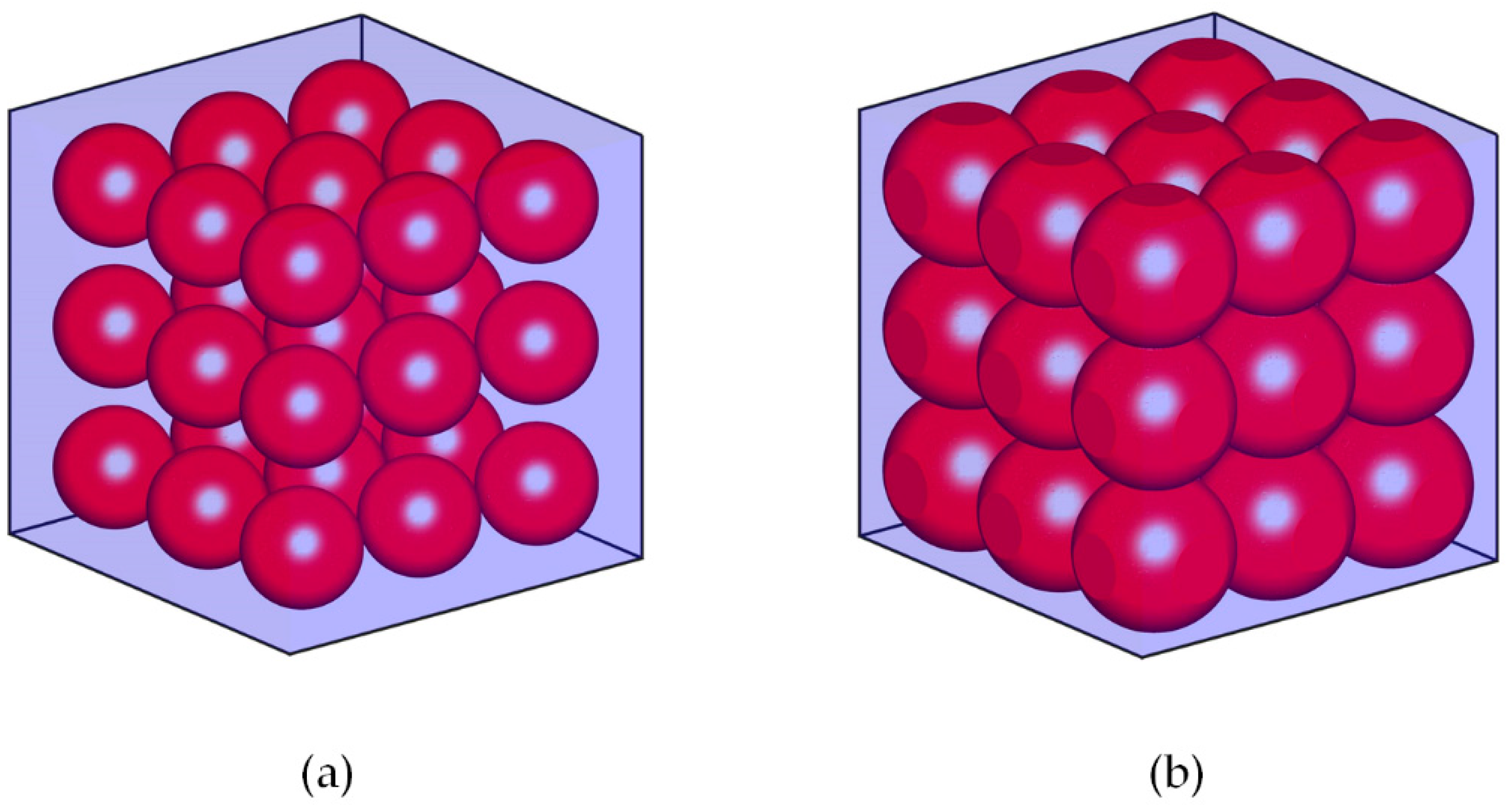
18]. Usually, equidistant domains around each node are used in MLPG implementations, with a radius around 60% of the local grid distance. Cubic integration domains around each node are used in the present 3D cases and, thus, the whole domain is covered without overlapping. During refinement in regions close to the interfaces, overlapping cannot be avoided without significant increase in the computational time. However, the overlapping is effectively restricted in small areas and does not affect the stability of the method. Figure 2 shows a domain comprising of a test sphere, Figure 2a, and the resulting computational grid, with integration sites around each node in the inlet, Figure 2b, consisting of cubes equal to the local grid spacing of each node. During numerical integration, one can have increased accuracy of the results either by increasing the order of the Gaussian quadrature integration, or by dividing the field of integration into smaller parts while keeping the integration order low. It was reported that the algorithm which computes integrals using subdivisions was more efficient than the one that integrates across the support domain with higher quadrature order [10,11]. Thus, the surface integrals for the cubic domains are calculated here as the sum of the integrals on the cube sides, and 3-point Gaussian quadrature is used in each side integral.
For heat conduction problems, it has been proven [18] that first-order interpolation is computationally efficient, fast and accurate. The optimal size of the support domain for the interpolation is ca 1.7 times the local grid spacing. The process of the grid generation, the construction of the shape functions, and the calculation of the integrals are performed here using Matlab kernels. The biconjugate gradient stabilized method (BiCGSTAB) [25] was used for the numerical solution of the resulting linear system.
For validation purposes, the thermal conductivity was calculated for various particulate systems using Comsol Multiphysics® and in-house developed automation Matlab® scripts for the generation of the CAD geometry. Once the geometry was created, the heat transport equation was solved using FE discretization (Galerkin approach), with free tetrahedral elements in the whole domain, and boundary layers (local refinement) developed along each side of the boundary interfaces. Details of the FE resolution are provided in the Section 5.

3. Simulation of Aggregate Formation

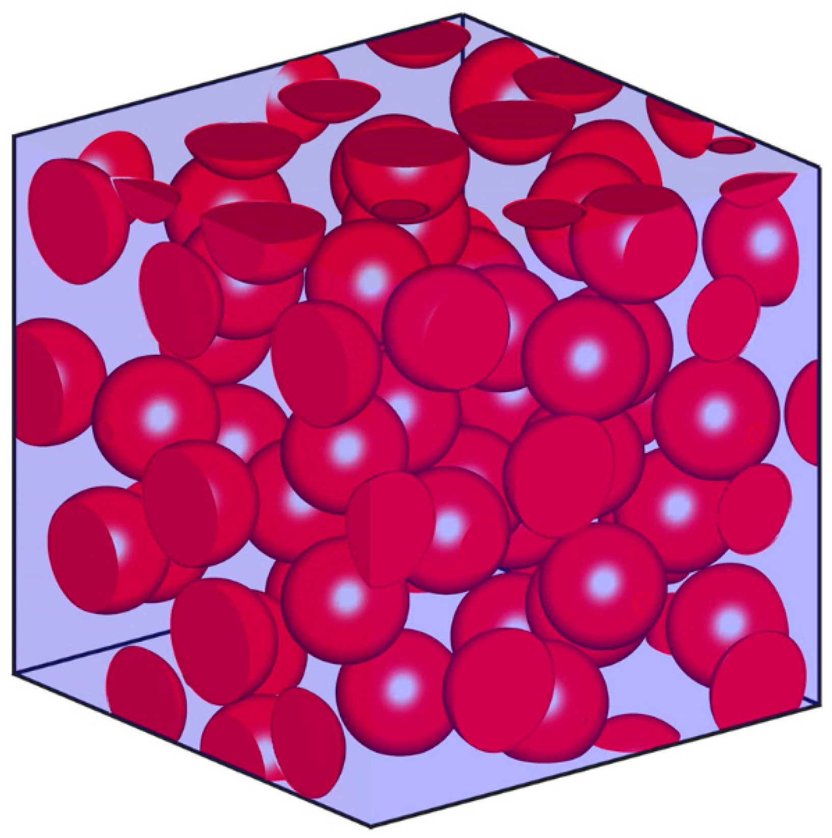
In the present work, the effective thermal conductivity of biphasic systems was calculated. Particularly, heat transport in particle systems and granular porous media was simulated. All the structures encompass a number of spheres within a cubic cavity. Algorithms based on Monte Carlo techniques were used to represent the particulate systems and granular porous media. Equally sized spheres were assumed, and the structures were periodic in every direction. The algorithm allowed random placement of the spheres over the working domain. The first, simple, case that was considered was that of granular media that were made up of spheres with no contact between them [26]. An example of a granular medium with porosity 0.7 is presented in Figure 3.
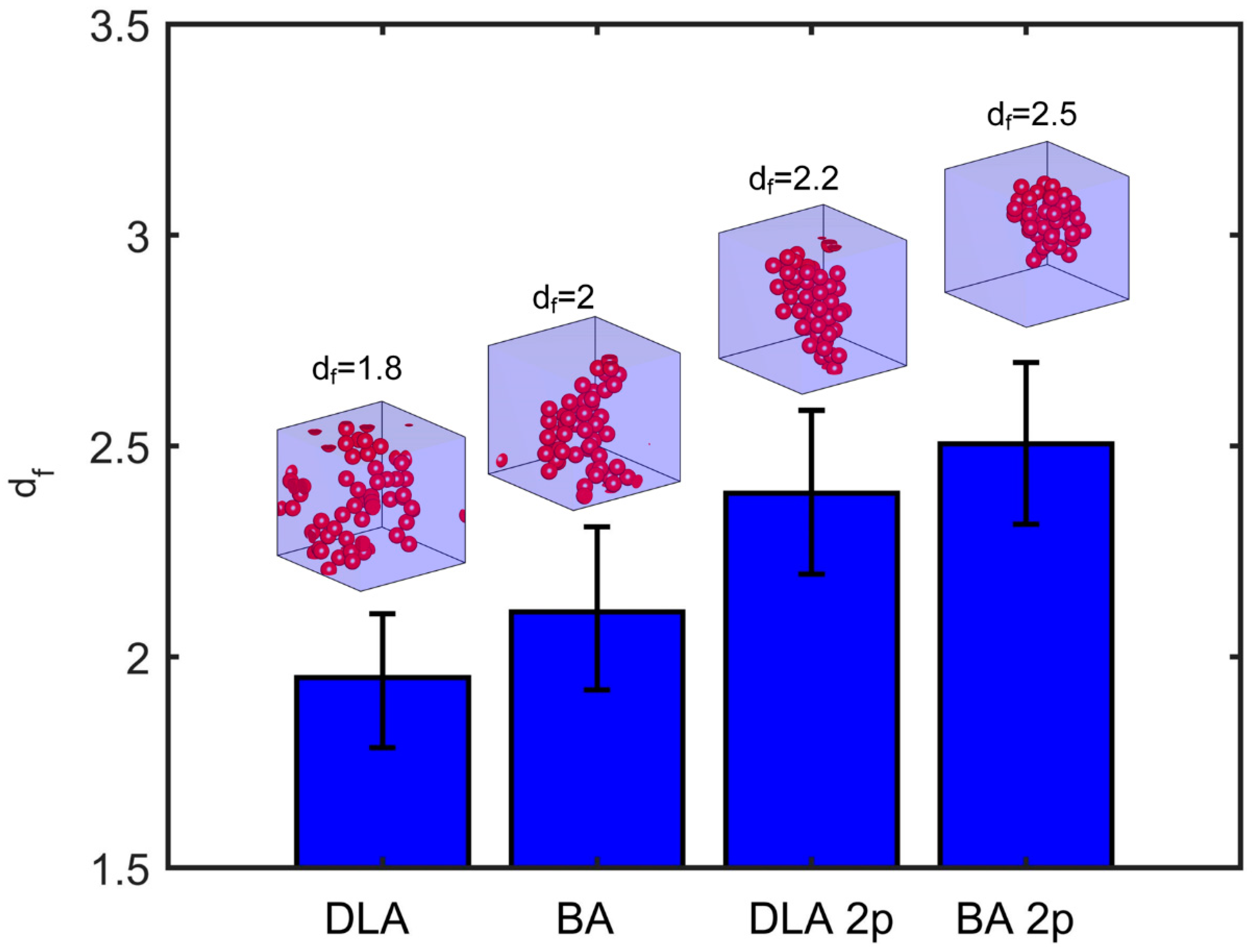
In addition, structures with aggregates of particles were simulated. In this case, every particle was in contact with at least another one. One of the determining parameters for the morphology of particle aggregates is their fractal dimension ( d f ) [27,28]. For an aggregate consisting of Ν particles, the fractal dimension ( d f ) relates the number of particles in the aggregate with its gyroscopic radius ( R g ), through: Ν ~ ( R g / r ) d f , where r is the radius of the particles. As a basic rule, one expects that the higher the fractal dimension, the more cohesive the aggregate.
For the representation of the aggregates, the well-known DLA [29] and the BA method [30] were used here, as well as modifications of these models, to represent denser aggregates. The DLA model describes the appropriate phenomena for the formation of fractal structures [29]. An important parameter of this method is the mean free path of the Brownian diffusion of particles [30]. If the mean free path is smaller than the size of the aggregate, the morphological characteristics of the clusters are the same and the fractal dimension is approximately d f ~ 1.9 . In the extreme case that the mean free path remains always larger than the aggregate size, the BA model is defined. The resulting aggregates are denser than those of the DLA model [30,31]. In these cases, every particle was assumed to cease its motion as soon as it gets in contact with another one. Extension of these models allows the particle to move along the surface of the cluster in order to find a suitable second contact point (DLA 2p, BA 2p) [30]. This method results in more compact aggregates. In Figure 4, the mean fractal dimension of 50 particles forming a single aggregate is presented along with its standard derivation for the DLA, BA, and their 2p counterpart aggregation methods. A visualization of aggregates resulting from each method is also shown accordingly.
The heat transport equation is solved in each of the aforementioned structures. The heat transfer is caused by the temperature difference imposed on the walls along the vertical axis. The rest of the boundaries are subject to periodic conditions.

4. Effective Medium Theory

Various models were proposed for the description of the thermal conductivity of a biphasic material. Most of the models of the effective medium theory type are based on the temperature distribution of a single spherical inclusion of one material in a matrix of another material [3],
T a n = { Q 0 · r ( 1 + k p k f k p + 2 k f ( R r ) 3 ) ,                             r > R Q 0 · r ( 1 + k p k f k p + 2 k f ) ,                                     r R ,
where R is the radius of the inclusion, r is the position vector emanating from the center of the sphere, Q 0 is a constant heat flux, and k p and k f are the thermal conductivity of the inclusion and the matrix, respectively. In the dilute limit, the effective thermal conductivity, k e f f , can be calculated [3] as
k e f f = k f + 3 k f k p k f k p + 2 k f f p ,
where f p is the volume fraction of the inclusion. Extending this result, Maxwell considered a set of spheres that do not interact with each other and, thus, the effective thermal conductivity was estimated from [3]
k e f f k f k e f f + 2 k f = f p k p k f k p + 2 k f .
Bruggeman calculated the perturbation in a homogeneous field due to the presence of particles and forced the sum of the perturbations to be zero. For two-phase systems the relationship is [3]
f p k p k e f f k p + 2 k e f f + ( 1 f p ) k f k e f f k f + 2 k e f f = 0 .
That expression is usually called self-consistent (SC). Bruggeman proposed a differential equation to predict the conductivity of biphasic systems. The differential effective medium approximation (DEM) is the solution of [3]
k p k e f f k p k f ( k f k e f f ) 1 / 3 = 1 f p .

5. Results and Discussion

5.1. Validation Model

For the verification of the accuracy of the proposed methods, the temperature distribution and the effective conductivity in a benchmark problem were calculated with the MLPG methods and compared with FD results. A solid sphere was placed at the center of a cubic domain with relative size corresponding to a volume fraction f p = 0.0042 . Dirichlet boundary conditions were applied for the temperature at all sides of the cube imposing heat flux in the vertical direction. The temperature distribution was obtained by the analytical solution of the problem of a single spherical inclusion in a matrix, Equation (9). The problem was then solved numerically with the FD and the MLPG methods. The MPLG method was used with the application either of the MLS approach, or of the DC PSE operators. Figure 5 shows the estimated error in the temperature profiles obtained by each method as a function of the total number of nodes. The error is defined as the weighted Euclidean norm of each approach and the analytical solution ( L 2 = n ( T i T a n ) 2 n , i = FD, MLPG). The comparison was made over a wide range of thermal conductivity ratios of the particle ( k p ) and the matrix ( k f ) , namely, between 0.01 and 100 .
The solution was attempted using normal grids, with relatively low uniform resolution ( 11 × 11 × 11 ), up to a relatively high one ( 81 × 81 × 81 ), with convergence at 10−6 precision globally. For cases with local refinement, grids of 11, 21, 41, and 81 nodes per dimension are used as initial density, with double resolution near the interfaces All the methods converge practically onto the analytical solution, as the maximum errors are of the order of 10 4 . For all k r cases, the MLPG method with local refinement converged at the same level of accuracy using one order of magnitude less nodes compared to FD ( 3 × 10 3 , 2 × 10 4 respectively, Figure 5d). This reduced substantially the computational cost. Moreover, the FD method showed higher errors in most cases.
The volume fraction of the particle was very small ( f p = 0.0042 ), so the effective conductivity could be accurately calculated from Equation (10) at the dilute limit. The superiority of the MLPG methods in view of their accuracy becomes more apparent in Figure 6, where the error on the effective thermal conductivity is presented. Local refinement clearly offers better description of the effective conductance.

5.2. Single Arrangement and Fully Dispersed Particles

The convergence of the numerical methods in a system of fully dispersed particles and in a single arrangement of spheres is examined in this section. The results of the meshless technique were validated with the output of the well-known, FE method-based, commercial software Comsol Multiphysics®.
In the case of fully dispersed particles, the particle number was set to one hundred (100) and their volume fraction f p to 0.1. The effective thermal conductivity of the system is presented in Figure 7 for varying discretization. The thermal conductivity ratio of the particles and the matrix was equal to k r = 0.01 , Figure 7a, and k r = 100 , Figure 7b. Figure 7 presents the convergence of the MLPG and the FE methods, as well as the predictions of Bruggeman’s DEM relationship, Equation (13). Regarding the discretization, the simulations start with a coarse grid of 31 nodes per dimension, i.e., ca. 3 × 10 4 total nodes, and reach a dense grid of 151 nodes per dimension ( 3.4 × 10 6 nodes in total). The methods with local refinement initially have a grid with 10 nodes per dimension, with a fourfold discretization near the interfaces, reaching 80 nodes per dimension and 5 × 10 6 total nodes. The results using a typical FE approach were in agreement with the predictions of the analytical expression and the meshless approach. Free tetrahedral elements were created and five boundary layers along the interfaces were used. The element size varied from 7% to 0.02% of the domain size for an extremely coarse and an extremely fine mesh, respectively. FE solutions converge up to 10 6 precision globally.
Initially, one can observe that the converged results of the simulations were very close to the predictions of the effective medium theory (EMT). Also, local refinement improved the solution in all cases. It is obvious that the use of MLPG with DC PSE and local refinement offered more stable description for the effective conductivity among the MLPG methods examined here.
The DC PSE with local refinement appears to have had practically the same convergence behavior as the FE method, having a minimum discretization of 50 nodes per dimension and total amount of nodes 5 × 10 5 , and provided a converged solution with an error less than 1%.
The thermal conductivity results for a single arrangement of spheres, Figure 8, are shown in Figure 9 for varying volume fraction of the inclusions. The MLPG method refers to the MLPG using the DC PSE operators and fourfold refinement near the interfaces. A grid with maximum resolution of 200 nodes per dimension proved sufficient for all cases. The problem was solved for a wide range of conductivity ratios. The simulations were in good agreement with the DEM approximation for low conductivity ratios, Figure 9a–c. In contrast, when the inclusions have much higher conductivity than the matrix ( k r = 100 ), Figure 9d, a steep increase of the effective conductivity in the region where f p = 0.524 was observed. At this volume fraction, a highly conductive path was created. This effect also appears in Figure 9c to a lower extent. This increase was not predicted by any of the EMT analytical models.
The commercial software package Comsol Multiphysics®, which is based on the FE approach, was used to evaluate the effective conductivity in the same particle system. For more advanced cases, where the closely packed spherical objects were interconnected, such as those in Figure 8b, special treatment from the user was required, due to the isolated or/and small regions that were created. This special case was the result of highly packed configurations of spherical objects, and the necessity for special numerical treatment was even more pronounced for real granular particles, which usually deviate from purely spherical shapes, Figure 8b. The approximation of the close packing of non-ideally spherical particles during reconstruction was achieved by allowing overlapping between the spheres to account for their closely-packed shape. Meshing of these intersected regions is usually characterized by increased difficulty, since the mesh generation at these areas is complicated. In addition, these small overlapped areas can be of the same order of magnitude as the minimum element size applied, which potentially leads to element-free spaces. To overcome this, the mesher generates a new finer mesh each time, eventually requiring a large number of elements and, consequently, a high computational cost. The software offers alternative options during the geometry construction, as well as in mesh generation procedure that can treat the overlapped areas. However, the treatment requires manual user input, which may further require trial and error processes. The latest software editions make this process easier; however, some difficulty in mesh construction was encountered when the geometry contained spheres whose surfaces are in contact or intersected with each other, as was the case of the aggregates of the present work.

5.3. Comparison with Experimental Data

The performance of the MLPG method with DC PSE and local refinement was compared with experimentally studied reference problems. In [32], the effective thermal conductivity of granular porous media was determined experimentally. Samples of sand were used, the void space of which was filled either with air or with water. During the present simulations, the structures were reconstructed using the Monte Carlo method, Figure 3. The mean radius of the sand is 0.9 mm with 10% deviation. The mean radius of 0.9 mm was used as the uniform particle radius for simulations. Figure 10a,b show the experimental data for the effective thermal conductivity as functions of the porosity ( 1 f p ) for the two fluids in the same porous medium. The thermal conductivity ratio of sand to water is 13, while that to air is 317. Each point represents the average results of 20 simulations with the same characteristics (porosity and ratio of thermal conductivities) and their standard deviation. Additionally, in this figure the predictions of the effective medium theory are shown. It is evident that the simulations coincide with the experimental data. Also, the DEM approach of the effective medium theory seems to predict adequately the conductivity. The SC approach appears to overestimate the result, while Maxwell’s approach underestimates it.
Figure 10c presents the effective thermal conductivity as a function of the conductivity ratio ( k r ). The experimental data were obtained from the same reference work [32], with behavior similar to the results with varying porosity. That is, the MLPG with the DC PSE method with local refinement near the interfaces produces results in excellent agreement with the experiments. DEM is also closer to the experimental data and the simulations than the rest of the analytical approaches studied here.

5.4. Effect of Aggregation on Thermal Conductivity

The convergence of the MLPG method in aggregate systems is shown in Figure 11 for two distinct structures resulting from convectional DLA and from DLA with two-point contact (DLA 2p) methods. In both methods the particle number was 20 and the volume fraction was f p = 0.05 , whereas their fractal dimension was 1.9 and 2.5, respectively. The insets of the figures show the percentage error versus the total number of nodes, assuming as base value the conductivity that was obtained for the maximum number of nodes. For conductivity ratio below unity ( k r = 0.01 ), convergence with errors less than 1% was achievable with coarse grids, having a few thousand nodes (~30 k) only, Figure 11a. In contrast, the cases of high thermal conductivity of the aggregates compared to that of the bulk ( k r = 100 ) were computationally demanding, Figure 11b. For coarse grids (30 k nodes) the error was between 10 and 20%, and the convergence depended on the fractal dimension. The lower the fractal dimension, the denser the grid required. For one million ( 10 6 ) nodes, the error for a dense aggregate ( d f = 2.5 ) was below 1%. For the same convergence, the DLA aggregate required 1.7 million nodes. This referred to a grid of 60 nodes per dimension in the bulk, locally refined at 240 nodes near the interfaces. Using this as a reference for grid-independent solutions, the effective conductivity dependence on the fractal dimension for 40 aggregated systems, 10 for each of the methods (DLA, BA, DLA 2p, BA 2p) is depicted in Figure 12 for a wide range of conductivity ratio values. For k r = 0.01 or k r = 0.1 the effective conductivity was practically independent of the fractal dimension of the particles, Figure 12a,b. The divergence of the results was less than 1%. However, when the conductivity of the particles was higher than that of the bulk, aggregation acts positively for the conduction. Indeed, it appears that the smaller the fractal dimension, the higher the thermal conductivity. The increase was small (~1%) for the cases of k r = 10 , though for strongly conductive particles ( k r = 100 ) a notable increase of 10% was observed. Moreover, it is noted that aggregates with the same fractal dimension resulting from different methods practically have the same effective conductivity.

6. Conclusions

A novel numerical method that combines the discretization-corrected particle strength exchange (DC PSE) operators with the meshless local Petrov–Galerkin (MLPG) technique was developed in order to simulate heat transport phenomena in particulate systems. Local refinement of the grid was shown to improve the accuracy of the calculations at reference geometries. An alternative, more efficient approach of interpolation was introduced, increasing the stability of the method and reducing the computational cost for grid construction. An automated method for grid refinement was introduced in multiple discretization levels inside the folds of the structures bypassing the necessity for user intervention. Moreover, the use of cubic domains to calculate local integrals, aiming at full geometry coverage with minimal overlapping, produced adequately stable and accurate results.
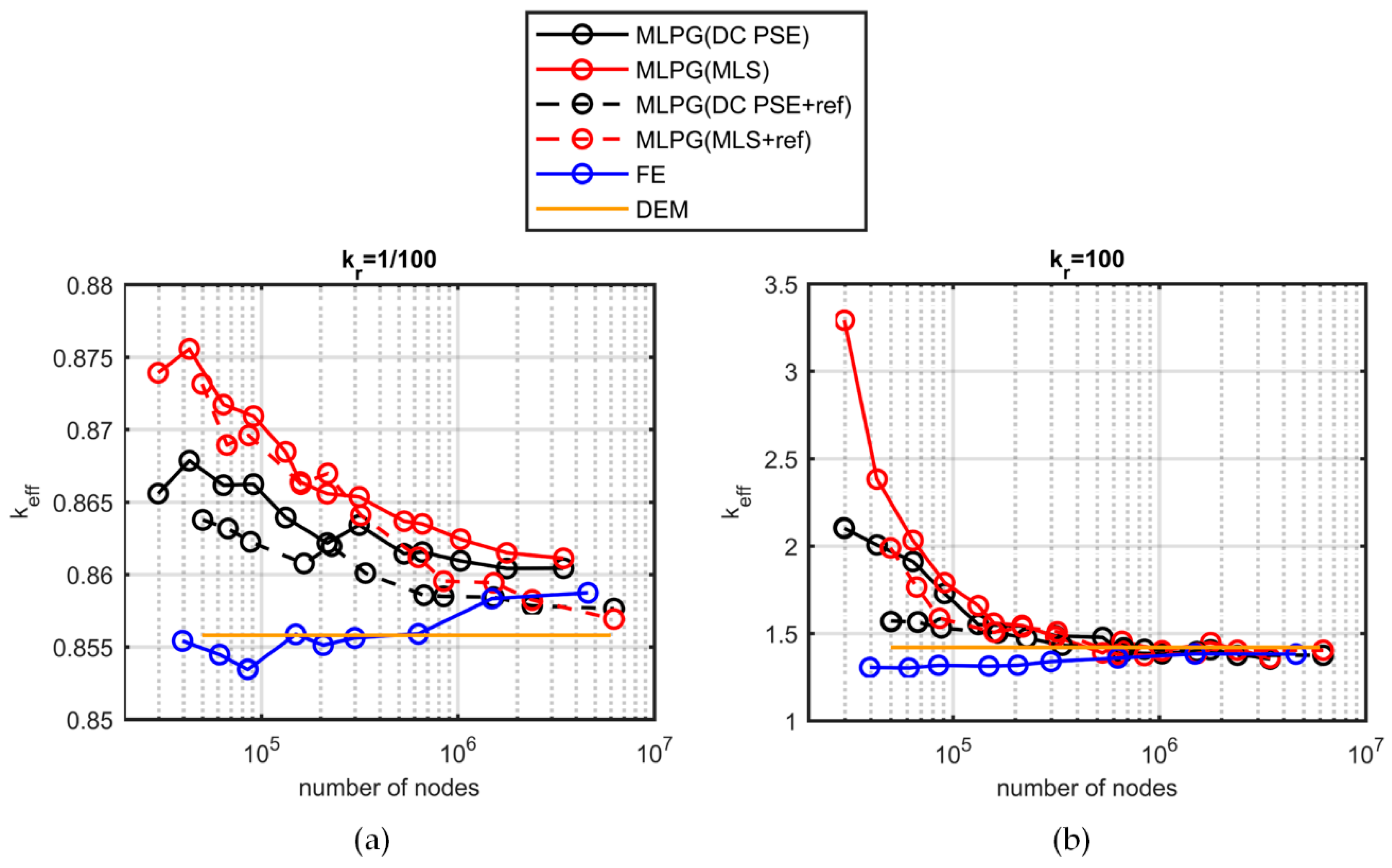
In addition, two different versions of the MLPG and the finite differences (FD) methods were compared in terms of the accuracy of the solutions. One version of the method used the moving least squares (MLS) approach for the trial function, while the other one used the DC PSE method. The DC PSE operators, which were used for the first time in this work as trial functions for the MLPG method, enhanced the solution stability and accuracy. It appears that the MLPG methods outweighed the FD one in the accuracy of the calculation for both the temperature distribution and the effective thermal conductivity. Additionally, the use of DC PSE operators reduced the computational cost required, as solutions converged using a smaller number of nodes.
The MLPG performance was tested against the performance of the finite element (FE) method-based software for the calculation of the effective conductivity in systems of fully dispersed spheres. The MLPG method with DC PSE operators and fourfold discretization near the interfaces had a convergence similar to that of the FE method. Experimental data from the literature were used for the sake of comparison with simulations. Sample structures were reconstructed with the Monte Carlo technique, and the heat transport problem was solved therein. The results of the MLPG method were in excellent agreement with experimental data. An important side outcome of this work is the observation that the differential effective medium (DEM) approximation predicted well the conductivity of unconsolidated granular media.
Finally, the convergence of the method for dense granular structures was studied, where the extension of particle overlapping significantly influenced the conduction, and therefore, the thermal conductivity. Aggregate structures with different morphological properties were reconstructed, and the effective conductivity was calculated with elevated accuracy, a result of great value in practical applications. For particles with conductivity lower than that of the bulk medium, the effective conductivity was not affected by aggregation, and the results were in full agreement with the Maxwell approximation. Conversely, for highly conducting particles, aggregation enhanced conduction. The thermal conductivity was a function of the fractal dimension of the aggregates. It was found that, as the fractal dimension decreased, the thermal conductivity increased monotonically.

Author Contributions

Conceptualization, N.P.K., E.D.S. and V.N.B.; methodology, N.P.K., N.B. and E.D.S.; software, N.P.K. and N.B.; supervision, V.N.B.; validation, N.P.K. and N.B.; visualization, N.P.K.; writing—original draft, N.P.K.; writing—review & editing, N.B., E.D.S. and V.N.B. All authors have read and agreed to the published version of the manuscript.

Funding

This research was funded by the Hellenic Foundation for Research and Innovation, PhD scholarships 2017 (HFRI, N. Karagiannakis), grant number 80264 and by the Stavros Niarchos Foundation within the framework of the project ARCHERS (“Advancing Young Researchers’ Human Capital in Cutting Edge Technologies in the Preservation of Cultural Heritage and the Tackling of Societal Challenges”).

Acknowledgments

Computational infrastructure was provided by the Institute of Chemical Engineering Sciences, Foundation for Research and Technology, Hellas (FORTH/ICE-HT).

Conflicts of Interest

On behalf of all authors, the corresponding author states that there are no conflicts of interest.

Abbreviations

BABallistic Aggregation
BiCGSTABBiconjugate gradient stabilized
DC PSEDiscretization-Corrected Particle Strength Exchange
DEMDifferential Effective Medium
DLADiffusion Limited Aggregation
EMTEffective Medium Approximation
FDFinite Differences
FEFinite Elements
MLPGMeshless Local Petrov–Galerkin
MLSMoving Least Squares
PSEParticle Strength Exchange
SCSelf-Consistent

References

  1. Bejan, A. Convection Heat Transfer; John Wiley & Sons: Hoboken, NJ, USA, 2013. [Google Scholar]
  2. Mahjoob, S.; Vafai, K. Analytical characterization of heat transport through biological media incorporating hyperthermia treatment. Int. J. Heat Mass Transf. 2009, 52, 1608–1618. [Google Scholar] [CrossRef]
  3. Torquato, S. Random Heterogeneous Materials: Microstructure and Macroscopic Properties; Springer Science & Business Media: Princeton, NJ, USA, 2013; Volume 16. [Google Scholar]
  4. Hashin, Z. Analysis of composite materials—A survey. J. Appl. Mech. 1983, 50, 481–505. [Google Scholar] [CrossRef]
  5. Batchelor, G. Transport properties of two-phase materials with random structure. Annu. Rev. Fluid Mech. 1974, 6, 227–255. [Google Scholar] [CrossRef]
  6. Cengel, Y.A.; Boles, M.A. Thermodynamics: An engineering approach. Sea 2002, 1000, 8862. [Google Scholar]
  7. Xiong, C.; Friedlander, S. Morphological properties of atmospheric aerosol aggregates. Proc. Natl. Acad. Sci. USA 2001, 98, 11851–11856. [Google Scholar] [CrossRef] [PubMed] [Green Version]
  8. Liu, G.-R. Meshfree Methods: Moving beyond the Finite Element Method; CRC Press: Boca Raton, FL, USA, 2009. [Google Scholar]
  9. Özişik, M.N.; Orlande, H.R.; Colaço, M.J.; Cotta, R.M. Finite Difference Methods in Heat Transfer; CRC Press: Boca Raton, FL, USA, 2017. [Google Scholar]
  10. Shen, S.N.A.; Sheng, P. The meshless local Petrov-Galerkin (MLPG) method: A simple & less-costly alternative to the finite element and boundary element methods. Comput. Model. Eng. Sci. 2002, 3, 11–51. [Google Scholar]
  11. Atluri, S.; Han, Z.; Rajendran, A. A new implementation of the meshless finite volume method, through the MLPG mixed approach. CMES: Comput. Model. Eng. Sci. 2004, 6, 491–514. [Google Scholar]
  12. Karagiannakis, N.; Bourantas, G.; Kalarakis, A.; Skouras, E.; Burganos, V. Transient thermal conduction with variable conductivity using the Meshless Local Petrov–Galerkin method. Appl. Math. Comput. 2016, 272, 676–686. [Google Scholar] [CrossRef] [Green Version]
  13. Bourantas, G.; Skouras, E.; Nikiforidis, G. Adaptive support domain implementation on the moving least squares approximation for mfree methods applied on elliptic and parabolic pde problems using strong-form description. Comput. Model. Eng. Sci. 2009, 43, 1–25. [Google Scholar]
  14. Cleary, P.W.; Monaghan, J.J. Conduction modelling using smoothed particle hydrodynamics. J. Comput. Phys. 1999, 148, 227–264. [Google Scholar] [CrossRef]
  15. Singh, I. A numerical solution of composite heat transfer problems using meshless method. Int. J. Heat Mass Transf. 2004, 47, 2123–2138. [Google Scholar] [CrossRef]
  16. Singh, I.; Prakash, R. The numerical solution of three dimensional transient heat conduction problems using element free Galerkin method. Int. J. Heat Tech 2003, 21, 73–80. [Google Scholar]
  17. Atluri, S.N.; Zhu, T. A new meshless local Petrov-Galerkin (MLPG) approach in computational mechanics. Comput. Mech. 1998, 22, 117–127. [Google Scholar] [CrossRef]
  18. Karagiannakis, N.P.; Bourantas, G.C.; Kalarakis, A.N.; Skouras, E.D.; Burganos, V.N. Efficiency of the meshless local Petrov-Galerkin method with moving least squares approximation for thermal conduction applications. Proc. AIP Conf. Proc. 2013, 2269–2272. [Google Scholar] [CrossRef]
  19. Wu, X.-H.; Tao, W.-Q. Meshless method based on the local weak-forms for steady-state heat conduction problems. Int. J. Heat Mass Transf. 2008, 51, 3103–3112. [Google Scholar] [CrossRef]
  20. Sladek, J.; Sladek, V.; Tan, C.; Atluri, S. Analysis of transient heat conduction in 3D anisotropic functionally graded solids, by the MLPG method. CMES: Comput. Model. Eng. Sci. 2008, 32, 161–174. [Google Scholar]
  21. Bourantas, G.; Petsi, A.; Skouras, E.; Burganos, V. Meshless point collocation for the numerical solution of Navier–Stokes flow equations inside an evaporating sessile droplet. Eng. Anal. Bound. Elem. 2012, 36, 240–247. [Google Scholar] [CrossRef]
  22. Schrader, B. Discretization-Corrected PSE Operators for Adaptive Multiresolution Particle Methods. Doctoral Thesis, ETH Zurich, Zurich, Switzerland, 2011. [Google Scholar]
  23. Bourantas, G.C.; Cheeseman, B.L.; Ramaswamy, R.; Sbalzarini, I.F. Using DC PSE operator discretization in Eulerian meshless collocation methods improves their robustness in complex geometries. Comput. Fluids 2016, 136, 285–300. [Google Scholar] [CrossRef] [Green Version]
  24. Eldredge, J.D.; Leonard, A.; Colonius, T. A general deterministic treatment of derivatives in particle methods. J. Comput. Phys. 2002, 180, 686–709. [Google Scholar] [CrossRef] [Green Version]
  25. Sleijpen, G.L.; Van der Vorst, H.A.; Fokkema, D.R. BiCGstab (l) and other hybrid Bi-CG methods. Numer. Algorithms 1994, 7, 75–109. [Google Scholar] [CrossRef] [Green Version]
  26. Bali, N.; Petsi, A.; Skouras, E.; Burganos, V. Three-dimensional reconstruction of bioactive membranes and pore-scale simulation of enzymatic reactions: The case of lactose hydrolysis. J. Membr. Sci. 2017, 524, 225–234. [Google Scholar] [CrossRef]
  27. Shih, W.Y.; Liu, J.; Shih, W.-H.; Aksay, I.A. Aggregation of colloidal particles with a finite interparticle attraction energy. J. Stat. Phys. 1991, 62, 961–984. [Google Scholar] [CrossRef]
  28. Weitz, D.; Oliveria, M. Fractal structures formed by kinetic aggregation of aqueous gold colloids. Phys. Rev. Lett. 1984, 52, 1433. [Google Scholar] [CrossRef]
  29. Witten, T., Jr.; Sander, L.M. Diffusion-limited aggregation, a kinetic critical phenomenon. Phys. Rev. Lett. 1981, 47, 1400. [Google Scholar] [CrossRef]
  30. Jullien, R. The application of fractals to colloidal aggregation. Croat. Chem. Acta 1992, 65, 215–235. [Google Scholar]
  31. Sorensen, C. The mobility of fractal aggregates: A review. Aerosol Sci. Technol. 2011, 45, 765–779. [Google Scholar] [CrossRef]
  32. Woodside, W.; Messmer, J. Thermal conductivity of porous media. I. Unconsolidated sands. J. Appl. Phys. 1961, 32, 1688–1699. [Google Scholar] [CrossRef]
Figure 1. Nodes contained in the support domain (red squares) of three representative nodes, located at the boundary of the refinement (red circles).
Applsci 10 00739 g001
Figure 2. (a) Initial geometry, (b) computational grid, and (c) integration domains around each node.
Applsci 10 00739 g002
Figure 3. Reconstruction of granular porous medium with solid volume fraction 0.3.
Applsci 10 00739 g003
Figure 4. Mean fractal dimension ( d f ) of 50 particles forming a single aggregate with the Diffusion Limited Aggregation (DLA) and Ballistic Aggregation (BA) methods, and their two-point contact (2p) counterparts, with their standard deviation, along with visualization of the corresponding aggregates.
Applsci 10 00739 g004
Figure 5. Weighted Euclidean norm of the deviation of the numerical approaches from the analytical solution as a function of the total number of nodes for conductivity ratio ( k r ) (a) 1/100 (b) 1/10, (c) 10, (d) 100. Red lines: MLPG with MLS. Black lines: MLPG with DC PSE. Continuous lines: normal grids. Dashed lines: grids locally refined. Blue lines: FD. Abbreviations: MLPG: meshless local Petrov-Galerkin, MLS: moving least squares, DC PSE: discretization-corrected particle strength exchange, FD: finite differences.
Applsci 10 00739 g005
Figure 6. Percentage error on the effective thermal conductivity as a function of the total number of nodes for 4 conductivity ratios ( k r ) (a) 1/100 (b) 1/10, (c) 10, (d) 100. Red lines: MLPG with MLS. Black lines: MLPG with DC PSE. Continuous lines: normal grids. Dashed lines: grids locally refined. Blue lines: FD. Abbreviations; MLPG: meshless local Petrov-Galerkin, MLS: moving least squares, DC PSE: discretization-corrected particle strength exchange, ref: local refinement, FD: finite differences.
Applsci 10 00739 g006
Figure 7. Effective thermal conductivity as a function of the total number of nodes for two different conductivity ratios ( k r ) (a) 1/100 (b) 100. Red lines: MLPG with MLS. Black lines: MLPG with DC PSE. Continuous lines: normal grids. Dashed lines: grids locally refined. Blue lines: FE. Abbreviations; MLPG: meshless local Petrov-Galerkin, MLS: moving least squares, DC PSE: discretization-corrected particle strength exchange, ref: local refinement, FE: finite element, DEM: differential effective medium approximation.
Applsci 10 00739 g007
Figure 8. Single arrangement of spherical particles. (a) f p = 0.3 , (b) f p = 0.7 .
Applsci 10 00739 g008
Figure 9. Effective thermal conductivity of the single arrangement as a function of the volume fraction of the inclusions for four different conductivity ratios ( k r ), (a) 1/100, (b) 1/10, (c) 10, (d) 100. Continuous lines: analytical expressions. Blue lines: Maxwell. Black lines: SC. Green lines: DEM. Dashed lines: simulations. Red: MLPG. Black: FE. Abbreviation; SC: self-consistent approximation, DEM: differential effective medium approximation MLPG: meshless local Petrov-Galerkin, FE: finite element.
Applsci 10 00739 g009
Figure 10. Effective thermal conductivity of a granular porous media as a function of the porosity for (a) k r = 13 , (b) k r = 317 . (c) Effective thermal conductivity of the granular medium as a function of the conductivity ratio. Circles: experimental data, Green lines: simulation results. Blue, Yellow and Red: Maxwell, DEM and SC models, respectively. Abbreviations; SC: self-consistent approximation, DEM: differential effective medium approximation MLPG: meshless local Petrov-Galerkin, exper: experimental data.
Applsci 10 00739 g010
Figure 11. Effective thermal conductivity as a function of the total number of nodes for two different aggregates. Red lines: d f = 2.5 . Black lines: d f = 1.9 . (a) k r = 0.01 . (b) k r = 100 . Insets: the percentage error. Abbreviation; DLA: diffusion limited aggregation.
Applsci 10 00739 g011
Figure 12. Effective thermal conductivity as a function of the fractal dimension for four different conductivity ratio ( k r ) values, (a) 1/100, (b) 1/10, (c) 10, (d) 100. Blue dots: BA. Red dots: DLA. Yellow dots: BA 2p. Purple dots: DLA 2p. Black lines: Maxwell model. Abbreviations; BA: ballistic aggregation, DLA: diffusion limited aggregation.
Applsci 10 00739 g012

