Abstract
In astronomy, physics, climate modeling, geoscience, planetary science, and many other disciplines, the mass of data often comes from spherical sampling. Therefore, establishing an efficient and distortion-free representation of spherical data is essential. This paper introduces a novel spherical (global) coordinate system that is free of singularity. Contrary to classical coordinates, such as Cartesian or spherical polar systems, the proposed coordinate system is naturally defined on the spherical surface. The basic idea of this coordinate system originated from the classical planar barycentric coordinates that describe the positions of points on a plane concerning the vertices of a given planar triangle; analogously, spherical area coordinates (SACs) describe the positions of points on a sphere concerning the vertices of a given spherical triangle. In particular, the global coordinate system is obtained by decomposing the globe into several identical triangular regions, constructing local coordinates for each region, and then combining them. Once the SACs have been established, the coordinate isolines form a new class of global grid systems. This kind of grid system has some useful properties: the grid cells exhaustively cover the globe without overlapping and have the same shape, and the grid system has a congruent hierarchical structure and simple relationship with traditional coordinates. These beneficial characteristics are suitable for organizing, representing, and analyzing spatial data.
1. Introduction
Astronomy, geoscience, computer graphics, and many other disciplines rely on research that uses spherical data. A fundamental problem lies in determining the optimal means of organizing, representing, or approximating these data. The most natural representation of spherical data is the spherical function or samples of the function f. Because of the intrinsic geometric properties of the sphere, the choice of an appropriate coordinate system is crucial for formulating an efficient and accurate numerical method for solving problems in spherical geometry. Spherical polar coordinates, although arguably the most natural coordinates for representing a point on a sphere , present several disadvantages (collectively known as pole problems) when used for numerical computations over the entire spherical surface. The other approach to representing data is to map the spherical domain onto a plane , such as the method used in traditional cartography. Then, points on a plane can be employed to process spherical signals. Unfortunately, in mathematics, the spherical surface is non-developable. That is, it is impossible to map a portion of the sphere onto the plane without introducing distortion (i.e., ’stretching’ or ’compressing’). For these reasons, a new class of spherical coordinates, spherical area coordinates (SACs), is presented in this paper. The SAC system is free of any singularity and naturally defined on the sphere surface, thus avoiding planar mapping distortion.
Research in science and engineering often needs a method for partitioning the sphere or some subset of it into sampling or analysis units (sphere tessellation or discretization). In geographical information systems (GISs), researchers have presented different kinds of Discrete Global Grid Systems (DGGSs) for organizing global data [1,2,3]. The most commonly used regular DGGSs are those based on the geographic (latitude–longitude) coordinate system. Raster global data sets often employ cell regions with the edges defined by arcs of equal-angle increments of latitude and longitude (for example, the and NASA Earth Radiation Budget Experiment (ERBE) grids [4] and National Geophysical Data Center (NGDC) 5-minute Gridded Earth Topography Data [5]). Grid systems based on the geographic coordinate system have numerous practical advantages. The geographic coordinate system is in line with people’s habits, and a wide array of existing data sets are based on it, so square grid regions are by far the most familiar to users. However, such grids have limitations: the cells of the grid become increasingly distorted in area, shape, and interpoint spacing as one moves north and south from the equator (Figure 1).
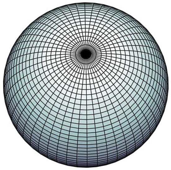
Figure 1.
The distortions of the geographical coordinate grid. The top and bottom row of grid cells are, in fact, triangles, not squares as they appear in the other row.
The north and south poles, both points on the surface of the globe, map to lines on the longitude × latitude plane. The top and bottom row of grid cells are, in fact, triangles, not squares as they appear in the other row. These polar singularities have forced applications, such as global climate modeling to make use of specific grids for polar regions. To solve these problems, researchers have proposed another kind of discrete global grid system called the Geodesic Global Grid System (Geodesic DGGS) [6], which is based on the geodesic dome invented by [7]. A geodesic dome is a spherical or partially spherical shell structure or lattice shell network on the surface of a sphere (Figure 2). These geodesic DGGSs are not a coordinate isoline grid but rather constructed by some specialized subdivision schemes [8].
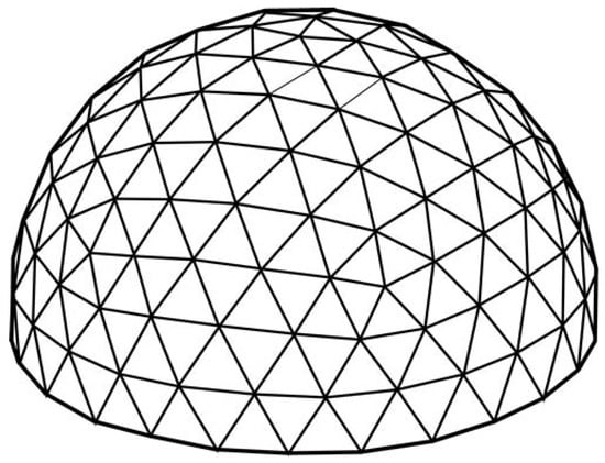
Figure 2.
Geodesic dome structure.
Furthermore, some of these grid systems have useful features, such as an equal-area hierarchical structure and regularity in shape. Rather than using great circle arcs for subdivision, Song et al. [9] proposed a small circle arc method that was optimized to achieve equal-area cell regions. However, the algorithms of some DGGSs are very complicated and have no analytical solution [1,3,9]. (In our approach, we have straightforward subdivision schemes and clear transformation laws between a spherical point’s Cartesian coordinate () and the SAC ().)
Global Grid Systems are widely used in different areas of science and engineering. The cubed sphere, a well-known Cartesian-to-spherical mapping, was proposed by Ronchi et al. [10] and has been used to solve partial differential equations on the sphere. On the basis of the same grid system, Simons et al. [11] proposed a class of spherical wavelet bases for the analysis of geophysical models and the tomographic inversion of global seismic data. Furthermore, an axis-free grid named the Yin-Yang grid was used by Wongwathanarat et al. [12] to simulate 3D self-gravitating flows. In computer graphics, researchers have developed some discrete spherical wavelet bases that rely on geodesic sphere construction [13,14,15,16,17]. They have been used successfully for spherical data visualization texturing and the bidirectional reflectance distribution function (BRDF).
In our approach, we adopt different strategies. First, we partition the globe into a series of spherical triangular cells without overlapping. Second, the local SACs on each triangular region are established, and then the global SACs can be constructed by gluing these local coordinate charts together along boundaries. Finally, we consider coordinate isolines to be grid cell edges and the intersection of isolines to be grid cell vertices, analogous to the Cartesian coordinate grid on a plane. The main properties of
- The construction process is very simple;
- Since our grid system has a slower growth rate between levels, it is more flexible and can be used for many applications;
- The grid cells have a low distortion in shape and area;
- The grid cells exhaustively cover the globe without overlapping;
- The grid system has a congruent hierarchical structure;
- The grid system has a simple relationship with conventional coordinates.
Our main contribution in this paper is the proposal of a new method to construct spherical area coordinates and a new kind of DGGS that is based on these coordinate systems.
2. Related Work
2.1. A Brief Review of the Geodesic DGGS
The following introductory paragraphs are intended to acquaint the reader with the concepts associated with the Geodesic DGGS.
A Discrete Global Grid (DGG) consists of a set of regions that form a partition of the sphere , where each region has a single point contained in the associated region. Each combination of a region and point is called a cell. A series of increasingly finer-resolution DGGs composes the DGGS. If the grids are defined consistently using regular planar polygons on a surrogate surface, the aperture of a DGGS is defined using the ratio of the areas of a planar polygon cell at resolutions k and [18]. The aperture of the system reflects the relationship between consecutive levels of the grids. Regular hierarchical relationships between DGGS resolutions play an important role in creating efficient data structures [19,20]. Two types of hierarchical relationships, congruent and aligned, are commonly used [6].
Consider to be a cell region and to be a cell point of a cell at resolution k.
- A DGGS is congruent if and only if
- A DGGS is aligned if and only if
If a DGGS does not have these properties, the system is defined as incongruent or unaligned.
In Sahr’s study [6], the construction of the Geodesic DGGS was treated as a series of design choices that were, for the most part, independent. The following five design choices fully specify a Geodesic DGGS:
- A base regular polyhedron;
- Polyhedron orientation;
- Subdivision scheme;
- Transformation;
- Choice of cell points.
2.1.1. Base Regular Polyhedron
The first step in the construction of a Geodesic DGGS is to establish an initial partition on the globe. Since multi-resolution discrete grids are obtained by subdividing the initial grid, the cells of the initial grid should preferably be the same regular spherical polygons. A geometrically rigorous solution to the problem of covering a spherical surface with tiles shows that there are only five classes of inscribed polyhedrons: the tetrahedron, the cube, the octahedron, the dodecahedron, and the icosahedron. All these polyhedrons produce a covering that is both regular and homogeneous. The covering can be obtained by a central projection of the sides and corners of the inscribed polyhedron on the spherical surface (Figure 3). These five platonic solids represent the only ways in which the sphere can be partitioned into cells, each consisting of the same regular spherical polygon, with the same number of polygons meeting at each vertex. Platonic solids have thus been commonly used to construct Geodesic DGGSs. In general, platonic solids with smaller faces reduce the distortion introduced when transforming between a face of the polyhedron and the corresponding spherical surface. The icosahedron is thus the most commonly chosen base regular polyhedron.
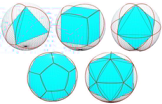
Figure 3.
Spherical tessellations of the five regular polyhedra.
2.1.2. Polyhedron Orientation
When a base polyhedron is chosen, a fixed orientation relative to the actual surface of the sphere must be determined. The best choice for the orientation of a base polyhedron mostly depends on the background. In geoscience, Fekete and Treinish [21] and Thuburn [22] placed a vertex of the icosahedron at each of the poles and then aligned one of the edges emanating from the vertex at the north pole with the prime meridian; this is the most common orientation. Fortunately, regardless of the chosen orientation, the geometric properties of the grid are not changed.
2.1.3. Subdivision Scheme
In the next step, we need to choose a method for subdividing this polyhedron to create multiple resolution grids. When the subdivision scheme has been chosen, one can partition a single face of the polyhedron or a set of faces that constitute a unit that tiles the polyhedron. A number of approaches to subdividing the surface of a polyhedron have been suggested, and the approaches can be classified according to different criteria. There are four types of subdivision schemes, and they have different partition shapes: triangles, squares, diamonds, and hexagons. Depending on the aperture of the grids, the approaches can be classified into two classes, namely, 4-fold and 9-fold. According to the kind of line that we use to connect the subdivision points, the approaches can be classified into two categories: Class I (connecting the subdivision points with lines parallel to the edges of the polyhedron face) and Class II (connecting the subdivision points with lines perpendicular to the edges of the polyhedron face). Figure 4 shows the most commonly chosen subdivision scheme for DGGSs.
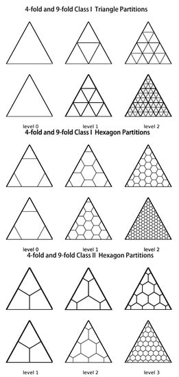
Figure 4.
Four- and 9-fold triangular and hexagonal partitioning of a single triangular face.
There are, however, other partition shapes. In this study, we investigated partitions that are based on the triangular face, but other partition shapes can be chosen.
2.1.4. Transformation
When choosing the partitioning method, we must select a method for creating a similar shape on the corresponding spherical surface. There are two types of approaches: Direct Spherical Subdivision (DSS) and Map Projection [20]. DSS approaches involve the creation of a partition directly on the spherical surface that maps to the corresponding partition on the planar face(s). The simplest direct subdividing method is using great circle arcs that correspond to the cell edges on the planar face(s). It should be noted that the aperture 4 Class I DSS is actually the geodesic bisector subdivision. This partitioning method has been used extensively to construct spherical wavelets [13,14,15,16]. Rather than using great circle arcs, Song et al. [9] proposed using small circle arcs that were optimized to achieve equal-area cell regions. Map projection approaches use an inverse map projection to transform a partition defined on the planar face(s) to the sphere. The most popular projections are the Gnomonic azimuthal projection, the Fuller Dymaxion projection [3,7], the Quaternary Triangular Mesh (QTM) [2,23], and the Snyder equal-area polyhedral projection.
2.1.5. Choice of Cell Points
Once the spherical grids have been specified, the points associated with the grid cells are usually chosen to be the center points of the cell regions. In map projection approaches, it is often convenient to choose the center points of the planar cell regions. In DSS approaches, the choice of the center points may be complicated.
2.2. Previous Work
Numerous spherical surface tessellations have been proposed to establish DGGSs. The most commonly used DGGS is the traditional latitude–longitude graticule, in which they are termed equal-angle grids. Another approach is the quadrilateral cells, which are called “constant-area” grids [24]. Constant-area tessellations begin with an arbitrarily sized quadrilateral cell at the equator and then define the parallel and meridian cell boundaries across the globe to achieve approximately equal-area cells. Fekete’s quad-tree data structure [21] and Song’s small circle subdivision [9] are both based on the recursive subdivision of spherical triangles obtained by projecting the faces of a regular polyhedron onto a sphere, and the edges of the cells are all great and/or small circle. The Hipparchus System [25] allows for the creation of arbitrarily regular DGGs by generating Voronoi cells on the surface of a sphere from a specified set of points. However, for many applications, it is desirable to have cells that consist of highly regular regions. The approaches discussed above are all a DSS, but there are some popular map projection methods. In the common Gnomonic azimuthal projection, all straight lines in the plane correspond to great circle arcs on the sphere but exhibit relatively large area and shape distortions and the geodesic bisector method give the same results. The Snyder equal-area polyhedral projection [1] is defined on all regular polyhedra, but it has greater shape distortion. The Dymaxion projection [7] given in [3] has less shape distortion than Snyder’s projection, and it is not an equal-area projection. Dutton’s Quaternary Triangular Mesh (QTM) [26] is based on the 4-fold recursive subdivision of the octahedron, and two projections have been proposed for transforming the QTM from the plane to the sphere: Goodchild and Yang’s Plate Carree projection [2] and Dutton’s Zenithial OrthoTriangular (ZOT) projection [23]. The difference between these two projections is that they use different planar surfaces. Dutton’s method uses an isosceles right triangle, and Goodchild and Yang’s method uses an equilateral triangle; however, both projections give identical geographic coordinates when taken to the sphere.
3. Spherical Area Coordinates (SACs)
Let us now more intuitively and visually introduce the basic concept that underlies the construction of the SAC system. The fundamental idea of our approach is inspired directly by F. Möbius’s work: barycentric coordinates [27].
3.1. Planar Area Coordinates
Let be a polygon with vertices . The barycentric coordinates of a point are continuous functions that satisfy the following properties for all points inside the polygon.
- ;
- ;
- .
Figure 5 illustrates the idea of barycentric coordinates for the case of planar triangles. Any point on the plane can be expressed by a linear combination of the vertices of the reference triangle : (property 3). The point outside the reference triangle can lead to negative coordinates, but this situation is not considered in this paper. Now, the question is, ’What are the continuous functions of the barycentric coordinates of point ?’ In the context of a triangle, barycentric coordinates are also known as area coordinates because the coordinates of with respect to the triangle are proportional to the areas of , and . The equations of area coordinates are written as
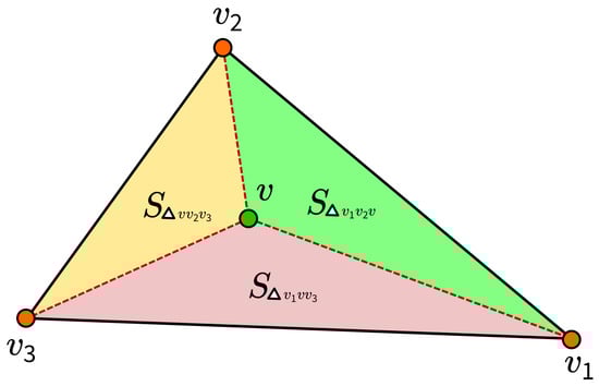
Figure 5.
Barycentric coordinates (in the case of planar triangles).
So, according to Equation (1), we can easily calculate the area coordinates of points , , and . The area coordinates of are
Since the triangles and are degenerate, the area of these two triangles is 0. As a result, the area coordinates of is . What is more, the area coordinates of the verties and are , and .
3.2. Local SACs
Spherical barycentric coordinates were first studied by Möbius [28] and introduced to computer graphics by Alfeld et al. [29]. In these papers, the spherical barycentric coordinates express the location of a point on a sphere to the vertices of a given spherical triangle P. In fact, Bronw and Worsey [30] showed that such coordinates that satisfy properties 1, 2, 3, just as planar barycentric coodinates, do not exist. Langer et al. [31] chose to relax property 2 to and to preserve property 3 because the main issue that they aimed to address was defining curves and surfaces over the sphere. Since our approach focuses on the problem of spherical surface tessellation, we chose different strategies: relax property 3 and preserve property 2.
3.2.1. Definition of SACs on the Spherical Triangle
In the context of SACs, the reference triangle is the spherical triangle T. The reference triangle can be any non-degenerate spherical triangle. Any area coordinates of the point in this reference triangle can be calculated through the vertices of this triangle. If there is a point inside T, then we can divide T into three sub-triangles by connecting and the vertices of the reference triangle with great circular arcs (see Figure 6a).
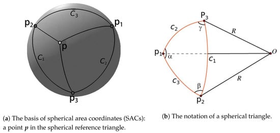
Figure 6.
SAC spherical reference triangle.
Definition 1.
A system of spherical area coordinates over a geodesic triangle T on is a one-to-one correspondence between points and ordered triples of real numbers such that
- 1.
- ;
- 2.
- ;
- 3.
- ,
where , , . It is obvious that the sub-triangles are all spherical triangles. Until this step, the coordinates of point can be written in the planar form (Equation (1)), but the issue lies in the method for calculating the areas of these four spherical triangles. Let a spherical triangle be drawn on the surface of a sphere of radius R, centered at a point (in Cartesian coordinates), with vertices , , and . Therefore, the vector from the center of the sphere to the vertices is given by , , and . We assume that the area of the spherical triangle is S, with . According to Girard’s theorem in spherical trigonometry, the area of a spherical triangle on a sphere of radius R is
where , , and denote the angles between the sides (dihedral angles) in radians (shown in Figure 6b), and the angle is opposite the side that subtends the greater circle arc , and so forth. Hence, the SACs can be written as
When the spherical reference triangle T is determined, the area of T is a constant, and , is a continuous function about the spherical point . According to cosine laws of spherical trigonometry,
The definitions of the dot product and cross-product are
Note that . Then, we obtain the formula below.
and so forth.
3.2.2. Transformation Laws between SACs and Cartesian Coordinates
Because Cartesian coordinates have been widely used in many areas of science and engineering, the transformation between Cartesian coordinates and SACs must be established. However, Equation (3) is too complicated for obtaining the transformation; thus, we need a simpler relationship between the spherical triangle area and its vertices. In spherical trigonometry, the following identity can be derived from sine and cosine laws [32]:
If the vectors in Equation (7) are given in the Cartesian coordinate system, then it determines the transformation rules from Cartesian coordinates to SAC.
Given a point P at , if the Cartesian coordinates of the vertices are known, then Equation (7) can be used to obtain
Finally, we obtain transformation laws between the Cartesian coordinates and SACs.
4. The Global SAC and Grid Systems
From the discussion above, the SACs are defined only in a portion of the sphere (inside the reference triangle). In other words, they are local coordinates. In this section, we introduce the extension of the SACs to the entire sphere. The first step is to partition the globe into several cells (the initial global grid), each consisting of the same regular spherical triangle. Further, the cells constitute a complete tiling of the globe, exhaustively covering the globe without overlapping. This criterion ensures that the sum of cell areas equals the surface area of the globe and that the coordinates of all shared cell edges are identical. Since cells of the initial global grid are spherical triangles, we can treat them as reference triangles and establish local SACs for each cell. When putting these patches together, we finally create a global coordinate system over the sphere. We expect that the initial global grid is regular. Since we require that the grid cells be a triangular cell, we now have only three options: the spherical tetrahedron, octahedron, and icosahedron versions. After the global SAC system has been developed, the coordinate grid naturally spans the globe.
4.1. The Tetrahedron Version of the Global Grid System
4.1.1. The Tetrahedron Version of SACs
For the first example, we show the development of the tetrahedron version of the SAC system. To acquire an elegant form of the transformation, we place the vertices of the tetrahedron at
The initial global grid consists of four equal-area spherical equilateral triangles, (shown in Figure 7), and the area is . Now, we use the method in Section 3.2 to establish the coordinates on each cell. The tetrahedron version of the SACs is an ordered tetrad of real numbers , and we specify that
Figure 7.
The tetrahedron version of the initial global grid.
Note that if the point lies on the edges of , then two of the coordinate components will be zero:
Finally, every point on the sphere corresponds to unique SACs .
To obtain the inverse transformations, we substitute into Equation (9) and solve the equation.
where and are third-order determinants:
4.1.2. The Tetrahedron Version of the Global Grid System
When a coordinate system is established on a surface (sphere/plane), some lines or curves must exist that can be represented by a constant value function. In a Cartesian coordinate system, can represent a horizontal line in the Euclidean plane, and if we choose a different value, the function will represent another horizontal line. When we choose some constant value as the step length , a serial of functions () represents a set of horizontal lines. Similar to these horizontal lines, functions () represent a set of vertical lines. These vertical and horizontal lines construct a coordinate grid at a certain resolution. In the geographic coordinate system, a set of parallels and meridians construct a coordinate grid on the Earth. Since we established the coordinate system on the sphere, there is a series of coordinate lines named the ultraviolet (UV)-isoline. In Figure 8, the green lines are the UV-isoline, and the expressions of these lines are . The black lines are the great circle arc that connects the midpoint of the reference triangle (red edges). The sub-regions that are subdivided by these two kinds of lines (UV-isoline and great circle arc) have different properties. The UV-isoline has smaller area and shape distortions.
Figure 8.
Ultraviolet (UV)-isoline and great circle arc.
Using these coordinates, one can easily construct the global grid by choosing a particular coordinate step length (), and the corresponding UV-isoline composes the network. We call this kind of global grid a UV-isogrid. In Figure 9, the values of are 1/2, 1/3, and 1/5. Figure 10 shows the 4-fold DGGSs based on SACs at levels 2, 3, and 4.
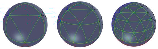
Figure 9.
The UV-isogrid .
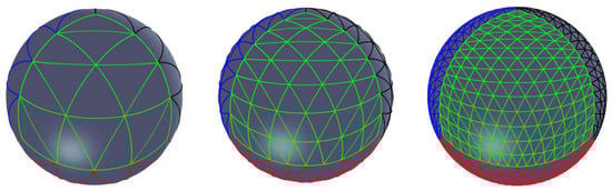
Figure 10.
The 4-fold tetrahedron version Discrete Global Grid Systems (DGGSs) based on SACs (level = 2, 3, 4).
4.2. The Octahedron Version of the Global Grid System
We can also define SACs on the octahedron. First, we need to orient the coordinate sphere triangles. The octahedron is oriented in the following way: the center of the sphere is at the coordinates , and the six vertices are at , , , , , and (shown in Figure 11).
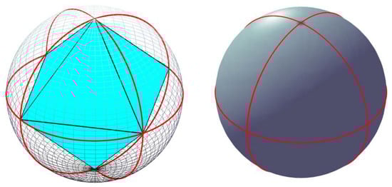
Figure 11.
The octahedron version of the initial global grid.
Then, we divide the sphere into eight spherical triangles. We denote these regions as (north) and (south), . Therefore, any point on the sphere surface must be in one of these eight cells, and the cells can serve as the reference triangle. Because the derivation is the same as the tetrahedron version, the forward transformation laws have the following forms:
Different from the tetrahedron version of SACs, the octahedron version of SACs have three components . In Equation (13), , , and are all positive. The SACs in different regions have different sign patterns and are determined by the regions containing the point P. The sign patterns are the same as the octants in the 3D Cartesian system (illustrated in Figure 12).
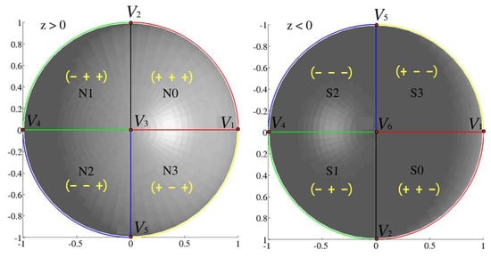
Figure 12.
The sign patterns of the octahedron version of SACs.
The inverse transformations are as follows:
where , , , and F are third-order determinants:
where , , and . Finally, according to the regions to which the point belongs, we assign the same sign patterns to the Cartesian coordinates :
and so forth. The main advantages of the octahedron version of SACs are that it has more symmetric coordinates than the tetrahedron version, and all regions share a unique equation. Figure 13 illustrates the octahedron version 4-fold DGGSs at levels 1, 2, 3, and 4.
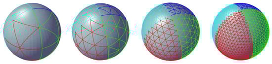
Figure 13.
Four-fold DGGSs based on the octahedron version of SACs (level = 1, 2, 3, 4).
4.3. The Icosahedron Version of the Global Grid System
The last version of SACs that we propose is based on the icosahedron. In this paragraph, we provide some visual examples of the icosahedron version of the global grid system and do not deduce the equations of the transformation again. The icosahedron orientation is as follows:
where
We define the icosahedron version of SACs with four components . The first three components are the coordinates of the spherical point, and the last component denotes the region to which the point belongs, that is, region (in Figure 14). Figure 15 illustrates three levels of DGGSs that are based on these coordinates.
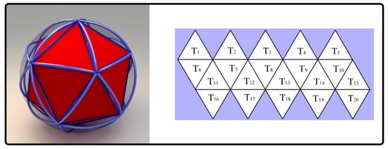
Figure 14.
The icosahedron version of the initial global grid and region index.
Figure 15.
Four-fold DGGSs based on the icosahedron version of SACs (level = 3, 4, 5).
4.4. Hexagonal Grid System
As we mentioned before, constructing a global grid system can use different partition method. There are two kinds of partition method: triangle partitions and hexagon partitions. In some disciplines, such as GIS, hexagonal global grid systems are more common and useful than triangular based grid systems. This subsection will give you some visual results that use SACs to create hexagonal based global grid. Figure 16 illustrates three levels of hexagonal based DGGSs that are based on SACs.
Figure 16.
Four-fold Class I Hexagon DGGSs based on the octahedron version of SACs (level = 4, 5, 6).
Hexagonal based grid has some advantages. They are more compact than triangles and squares and also have the smallest average error. Because hexagons are more symmetry, they provide the highest angular resolution. Unlike square and triangle grids, hexagon grids have uniform adjacency; each hexagon cell has six neighbors. But the hexagonal based grids also have some disadvantages. The grid’s cells are not all hexagon, some pentagons exist in the initial vertices of Platonic solid. A simple data structure, like quadtrees, octrees cannot use to index the grid systems. In this paper, we focus on triangular based grid systems.
5. Results
5.1. DGGS Evaluation Criteria
When there is a new global grid, a common question arises: What is the difference between this grid and existing ones? What are the advantages of this grid? Some researchers have proposed a series of standards for evaluating global spherical grids. These standards include the following:
- The grid cells complete tiling the globe without overlapping in any resolution;
- The grid cells at one resolution have equal areas;
- The grid cells have the same topology;
- The grid cells have the same shape;
- The grid system has a simple relationship with the latitude and longitude graticule;
- The grid system contains grids of any defined spatial resolution;
- The grid cells are compact.
Table 1 gives the result between different methods based on the criteria.

Table 1.
Criteria comparison between different methods.
5.2. Performance Analysis
We compared the performance of different DGGSs by measuring two general properties: area and shape distortions. We used the perimeter and area as the two direct measurements of partition cells. Since the edges of the partition cells are not always great circle arcs in all methods, we used an approximation method to compute the perimeter and area of the partition cells. At all levels of subdivision, we calculated the resolution of representation as not instantly level but level of the partition cells. A large number of flat triangular facets approximate a spherical triangle. We calculated the perimeters as the sum of the lengths of straight lines, and we calculated the area as the sum of the area of small planar triangles. For each comparison, we started with a set of partition cells on the sphere that were generated from one of the three polyhedrons, one of the two density ratios, one of four methods (including our approach) for mapping to the sphere, and one of the eight or five levels of recursion, depending on the density ratio.
For a more natural interpretation of the comparisons, we used standardized measures. For area measurements, we converted the actual areas to regulated areas for each level of recursion by dividing the exact areas by the values listed in Table 2 to obtain regions relative to a unit value of 1. For shape measurements, we used a standardized perimeter-to-area ratio and called this the ‘Zone Standardized Compactness’ (ZSC) [20] using the equation below.
where a is the cell area, p is the cell perimeter, and r is the radius of the sphere. The resulting values were then dimensionless numbers between 0 and 1.
Table 2.
Cell counts and standardized surface areas for DGGSs based on a single face of the spherical tetrahedron, octahedron, and icosahedron.
In this subsection, we compare the distortion performance of our approach with that of some classical DGGSs. We implemented two recursive partitioning methods (4-fold, 9-fold) and three methods of mapping the partition from the polyhedron to the surface of the sphere. These three methods are the Snyder projection method, the geo bisector (geodesic bisector) method, and the Dymaxion projection. All these global partitions are based on the tetrahedron, octahedron, and icosahedron.
5.3. Measures of Performance
Figure 17 provides the visual results of the four DGGSs based on different methods. Our DGGSs have, on average, the most compact cells and smaller area distortions, except for the Snyder equal-area DGGSs. Since equivalent surface areas for the cells are maintained, Snyder’s DGGSs exhibit more shape distortions, especially in the cells along the radial lines that extend from a polyhedron face center to its vertices.
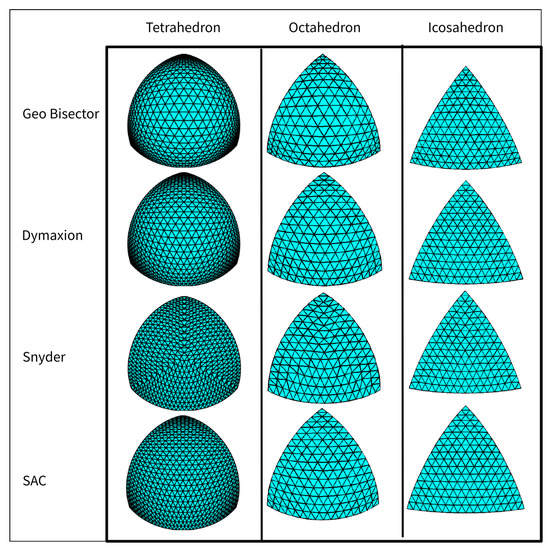
Figure 17.
The four polyhedral DGGSs. Each figure shows a 4-fold, level-5 triangle subdivision on polyhedrons. The surfaces are shown in an orthographic projection to accentuate the distortion patterns present in each method.
We used five statistics of shape and area measurements: the range of the different area (standardized area), the standard deviation of the area, the range of compactness, the standard deviation of compactness, and the mean compactness. Figure 18, Figure 19 and Figure 20 illustrate the performance of DGGSs by the level of resolution for each of the five response measures.
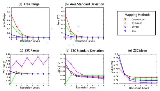
Figure 18.
Graphs of the five statistics of the area and Zone Standardized Compactness (ZSC) response measurements for each method as a sequence by recursion level (level 1 to level 8). These results are for the tetrahedron using the 4-fold density ratio.
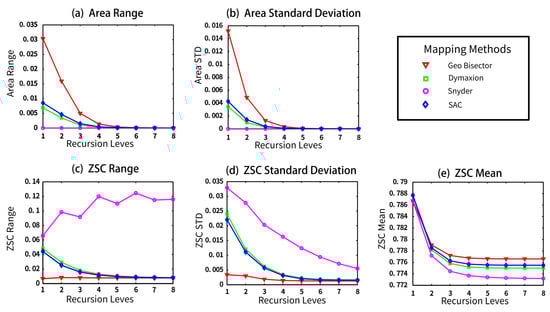
Figure 19.
Graphs of the five statistics of the area and ZSC response measurements for each method as a sequence by recursion level (level 1 to level 8). These results are for the icosahedron using the 4-fold density ratio.
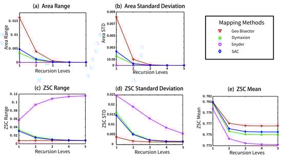
Figure 20.
Graphs of the five statistics of the area and ZSC response measurements for each method as a sequence by recursion level (level 1 to level 5). These results are for the icosahedron using the 9-fold density ratio.
Differences in the range of the area distortion in the different methods are clearly distinguished as the resolution increases (shown in Figure 18a, Figure 19a, Figure 20a). The greatest area distortion is found with the Geo Bisector method, followed by (in descending order) the Dymaxion projection method, SACs, and Snyder. The Snyder projection has an area range of zero, of course, since it is an equal-area mapping method.
For the compactness measures, the Snyder method has the highest scores both in range and standard deviation (Figure 18c, Figure 19c, Figure 20c). These results indicate that the Snyder equal-area projection has the most shape distortion. The compactness performance of our method is almost the same as that of the Dymaxion method. As the mean of the compactness increases, it approaches the most compact shape possible. The results of the experiments for this measure show that the Geo Bisector has the best performance (highest values).
The histograms of the distributions of the area bias and compactness values (in Figure 21 and Figure 22) show distinct differences between methods. The Snyder projection histogram for the area has only one bar for the single equal-area value (no bias). Our method has a continuous, unimodal histogram. It also has a better shape distortion performance than the Dymaxion and Geo Bisector methods on the tetrahedron (Figure 21a). For the icosahedron, no matter what fold method is used the histogram for our method has a smoother distribution (Figure 22a andFigure 23a).
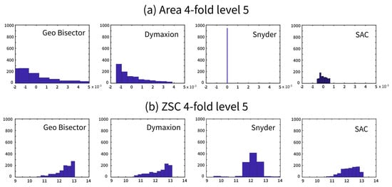
Figure 21.
The distribution histograms of area and compactness for different methods. These values are for the tetrahedron partitions.
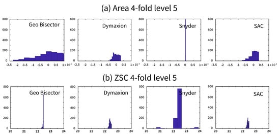
Figure 22.
The distribution histograms of area and compactness for different methods. These values are for the icosahedron partitions.
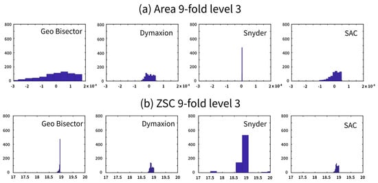
Figure 23.
The distribution histograms of area and compactness for different methods. These values are for the icosahedron partitions.
The maps of the spatial variation in the area and ZSC values have interesting patterns (in Figure 24, Figure 25 and Figure 26). For the 4-fold density ratio, the spatial variation in the area (Figure 24a and Figure 25a) has one of two patterns. The Snyder method result is homogeneous with an equal area. The other three methods created partitions with a decrease in area per cell radially from the center. For compactness, each method has a unique pattern (in Figure 24b and Figure 25b). For the 9-fold density ratio, all methods have patterns of area and compactness variation that are very similar to those for the 4-fold ratio (in Figure 26).
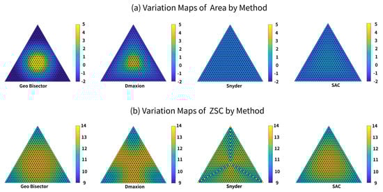
Figure 24.
Maps of the spatial variation in the area and ZSC measurements for the Geo Bisector, Snyder, Dymaxion, and SAC methods for the tetrahedron and 4-fold density ratio.
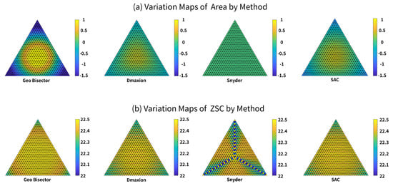
Figure 25.
Maps of the spatial variation in the area and ZSC measurements for the Geo Bisector, Snyder, Dymaxion, and SAC methods for the icosahedron and 4-fold density ratio.
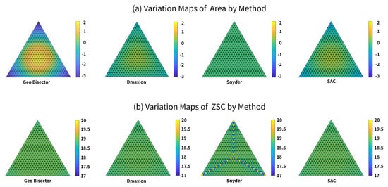
Figure 26.
Maps of the spatial variation in the area and ZSC measurements for the Geo Bisector, Snyder, Dymaxion, and SAC methods for the icosahedron and 9-fold density ratio.
6. Discussion
This paper presents several complementary views of the distortion performance of different methods for partitioning the triangular faces of polyhedrons. These views show that our method has a generally smoother distribution in both area and shape measurements, especially for the tetrahedron. Another key advantage of our method is not only the association of points but also the continuous functions with the cells. In classical DGGSs, each cell can only associate with one point. If more than one point needs to be represented, a higher-resolution DGGS is required.
7. Conclusions and Further Work
In this paper, we detail a method for defining SACs on the globe. Further, we compare our approach with some classical DGGS methods. We also compare the performance between SAC DGGSs and three classical DGGSs. The analysis results illustrate that the DGGSs based on SACs have an average performance. This means that they have small area and shape distortions simultaneously. Another advantage is the explicit transformation equation between the Cartesian coordinates and SACs.
We show that the SAC system is a global coordinate system and can be used to represent different kinds of spherical signals: continuous function (Figure 27) and discrete sampling data (Figure 28). On the other hand, contrary to many other approaches, such as the methods of [1,9], the transformations between Cartesian coordinates and SACs are analytical and compact. Because the global grid system constructed by our method is triangular, techniques that have been proposed for processing the triangular grid [33] can also be used to deal with our system.
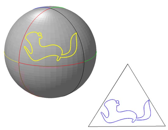
Figure 27.
The shape of the squirrel is composed of 10 parametric curves (equations). In the planar triangle, there is the planar version of the curves that use the same form of expressions as the spherical version.
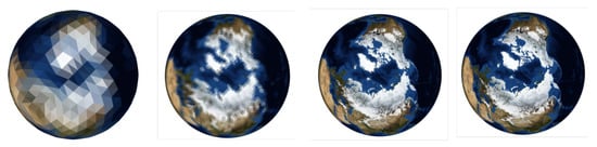
Figure 28.
The discrete Earth data visualization based on the octahedron version of global SACs. Resolution level = 4, 6, 8, 10.
It would be interesting to establish a general theory of SACs for spherical signal processing. Could the SACs be used in spherical CAGD (Computer Aided Geometric Design) or solve partial differential equations in spherical geometry? Another future work is how to describe the surface with a single binary number. Using the binary description it would be much more computationally efficient to calculate gradients, etc. These topics need exploration in future studies.
Author Contributions
Conceptualization, K.L. and D.Q.; methodology, K.L. and D.Q.; software, K.L.; writing—original draft preparation, K.L.; writing—review and editing, K.L. and X.T.; visualization, K.L. All authors have read and agreed to the published version of the manuscript.
Funding
This research was funded by The Science and Technology Development Fund, Macau SAR (File No. 099/2016/A3).
Conflicts of Interest
The authors declare no conflicts of interest.
Abbreviations
The following abbreviations are used in this manuscript:
| 3D | Three Dimensional |
| BRDF | Bidirectional Reflectance Distribution Function |
| DGGS | Discrete Global Grid System |
| ERBE | Earth Radiation Budget Experiment |
| GIS | Geographical Information System |
| NGDC | National Geophysical Data Center |
| SAC | Spherical Area Coordinate |
| SACS | Spherical Area Coordinate System |
| ZSC | Zone Standardized Compactness |
| CAGD | Computer Aided Geometric Design |
References
- Snyder, J.P. An equal-area map projection for polyhedral globes. Cartographica 1992, 29, 10–21. [Google Scholar] [CrossRef]
- Goodchild, M.F. A Hierarchical spatial data structure for global geographic information systems. CVGIP Gr. Models Image Process. 1992, 54, 31–44. [Google Scholar] [CrossRef]
- Gray, R.W. Exact transformation equations for Fuller’s world map. Cartogr. Geogr. Inf. Syst. 1994, 21, 243–246. [Google Scholar] [CrossRef]
- Brooks, D.R. Grid Systems for Earth Radiation Budget Experiment Applications; Technical Report 83233; NASA-LRC: Hampton, VA, USA, 1981.
- Hastings, D.; Dunbar, P. Development and assessment of the global one-km base elevation digital elevation model (GLOBE). ISPRS Arch. 1998, 32, 218–221. [Google Scholar]
- Sahr, K.; White, D.; Kimerling, A. Geodesic discrete global grid systems. Cartogr. Geogr. Inf. Sci. 2003, 30, 121–134. [Google Scholar] [CrossRef]
- Fuller, R.B. Synergetics; MacMillan: New York, NY, USA, 1975. [Google Scholar]
- White, D.; Kimerling, A.J.; Sahr, K.; Song, L. Comparing area and shape distortion on polyhedral-based recursive partitions of the sphere. INT. J. Geograp. Inf. Sci. 1998, 12, 805–827. [Google Scholar] [CrossRef]
- Song, L.; Kimerling, A.J.; Sahr, K. Developing and equal area global grid by small circle subdivision. In Descrete Global Grids a Web Book; GoodChild, M.F., Kimerling, A.J., Eds.; 2002; Available online: http://www.geo.upm.es/postgrado/CarlosLopez/materiales/cursos/www.ncgia.ucsb.edu/globalgrids-book/song-kimmerling-sahr/ (accessed on 10 January 2020).
- Ronchi, C.; Iacono, R.; Paolucci, P.S. The ’Cubed Sphere’: A new method for the solution of partial differential equations in spherical geometry. J. Comput. Phys. 1996, 124, 93–114. [Google Scholar] [CrossRef]
- Simons, F.J.; Loris, I.; Nolet, G.; Daubechies, I.C.; Voronin, S.; Judd, J.S.; Vetter, P.A.; Charlety, J.; Vonesch, C. Solving or resolving global tomographic models with spherical wavelets, and the scale and sparsity of seismic heterogeneity. Geophys. J. Int. 2011, 187, 969–988. [Google Scholar] [CrossRef]
- Wongwathanarat, A.; Hammer, N.J.; Müller, E. An axis-free overset grid in spherical polar coordinates for simulating 3D self-gravitating flows. Astron. Astrophys. 2010, 514, A48. [Google Scholar] [CrossRef]
- Schröder, P.; Sweldens, W. Spherical wavelets: Efficiently representing functions on the sphere. In Proceedings of the 22nd Annual Conference on Computer Graphics and Interactive Techniques (SIGGRAPH ’95); ACM: New York, NY, USA, 1995; pp. 161–172. [Google Scholar]
- Schröder, P.; Sweldens, W. Spherical Wavelets: Texture Processing; Technical Report 1995:4; Industrial Mathematics Initiative, Department of Mathematics, University of South Carolina: Columbia, SC, USA, 1995. [Google Scholar]
- Bonneau, G.P. Optimal triangular Haar bases for spherical data. In Proceedings of the Conference on Visualization’99: Celebrating Ten Years, San Francisco, CA, USA, 24–29 October 1999; pp. 279–284. [Google Scholar]
- Nielson, G.; Jung, I.H.; Sung, J. Haar wavelets over triangular domains with aplications to multiresolution models for flow over a sphere. In Proceedings of the 8th Conference on Visualization ’97, Phoenix, AZ, USA, 19–24 October 1997; pp. 143–149. [Google Scholar]
- Lessig, C.; Fiume, E. SOHO: Orthogonal and symmetric Haar wavelets on the sphere. ACM Trans. Graph. 2008, 27, 4:1–4:11. [Google Scholar] [CrossRef]
- Bell, S.B.; Diaz, B.M.; Holroyd, F.; Jackson, M.J. Spatially referenced methods of processing raster and vector data. Image Vis. Comput. 1983, 1, 211–220. [Google Scholar] [CrossRef]
- Clarke, K.C.; GoodChild, M.F.; Kimerling, A.J. Criteria and measures for the comparison of global geocoding systems. In International Conference on Discrete Global Grids; Elsevier: Santa Barbara, CA, USA, 2002; pp. 26–28. [Google Scholar]
- Kimerling, A.J.; Sahr, K.; White, D.; Song, L. Comparing geometrical properties of global grids. Cartogr. Geogr. Inf. Sci. 1999, 26, 271–287. [Google Scholar] [CrossRef]
- Fekete, G.; Treinish, L.A. Sphere quadtrees: A new data structure to support the visualization of spherically distributed data. In Extracting Meaning from Complex Data: Processing, Display, Interaction; International Society for Optics and Photonics: Bellingham, WA, USA, 1990; Volume 1259, pp. 242–253. [Google Scholar]
- Thuburn, J. A PV-based shallow-water model on a hexagonal-icosahedral grid. Mon. Weather Rev. 1997, 125, 2328–2347. [Google Scholar] [CrossRef]
- Dutton, G. Zenithial OrthoTriangular Projection; Proc. Auto-Carto 10; ASPRS: Bethesda, MD, USA, 1991; pp. 77–95. [Google Scholar]
- Kahn, R. What Shall We Do with the Data We are Expecting in 1998? Proceedings of the Massive Data Sets Workshop; The National Academies Press: Washington, DC, USA, 1996; pp. 15–21. [Google Scholar]
- Lukatela, H. Hipparchus geopositioning model: An overview. In Proceedings of the Auto Carto 8 Symposium, Baltimore, MD, USA, 29 March–3 April 1987; pp. 87–96. [Google Scholar]
- Dutton, G. Geodesic modeling of planetary relief. Cartographica 1984, 21, 188–207. [Google Scholar] [CrossRef]
- Möbius, A.F. Der barycentrische calcul. Johann Ambrosius Barth. 1827. Available online: https://books.google.com.hk/books?hl=en&lr=&id=aM9UAAAAcAAJ&oi=fnd&pg=PA3&dq=M%C3%B6bius,+A.F.+Der+barycentrische+calcul.+Johann+Ambrosius+Barth+1827&ots=FJMEk1oPL9&sig=-PM6w5urDe-mFE3Ba_UoiQgEsDc&redir_esc=y&hl=zh-CN&sourceid=cndr#v=onepage&q=M%C3%B6bius%2C%20A.F.%20Der%20barycentrische%20calcul.%20Johann%20Ambrosius%20Barth%201827&f=false (accessed on 8 January 2020).
- Möbius, A.F. Ueber eine neue Behandlungsweise der analytischen Sphärik. Abhandlungen bei Begründung der Königl. Sächs. Gesellschaft der Wissenschaften 1846, 45–86. Available online: https://books.google.com.br/books?id=X3oVw_WTCpYC&pg=PA120-IA1&lpg=PA120-IA1&dq=M%C3%B6bius,+A.F.+Ueber+eine+neue+Behandlungsweise+der+analytischen+Sph%C3%A4rik.+Abhandlungen+bei+Begr%C3%BCndung+der+K%C3%B6nigl.+S%C3%A4chs.+Gesellschaft+der+Wissenschaften+1846&source=bl&ots=72aRY44pzw&sig=ACfU3U3zrThn_2-k-IQD9DEnEzsEn9sfdA&hl=zh-CN&sa=X&ved=2ahUKEwiVv7nS7YfnAhXCFIgKHQsnD84Q6AEwAHoECAQQAQ#v=onepage&q=M%C3%B6bius%2C%20A.F.%20Ueber%20eine%20neue%20Behandlungsweise%20der%20analytischen%20Sph%C3%A4rik.%20Abhandlungen%20bei%20Begr%C3%BCndung%20der%20K%C3%B6nigl.%20S%C3%A4chs.%20Gesellschaft%20der%20Wissenschaften%201846&f=false (accessed on 8 January 2020).
- Alfeld, P.; Neamtu, M.; Schumaker, L.L. Bernstein-Bézier polynomials on spheres and sphere-like surfaces. Comput. Aided Geom. Des. 1996, 13, 333–349. [Google Scholar] [CrossRef]
- Bronw, J.; Worsey, A. Problems with defining barycentric coordinates for the sphere. RAIRO Modélisation Mathématique et Analyse Numérique 1992, 26, 37–49. [Google Scholar]
- Langer, T.; Belyaev, A.; Seidel, H.P. Spherical barycentric coordinates. In Proceedings of the 4th Eurographics Symposium on Geometry Processing (SGP ’06), Cagliari, Italy, 26–28 June 2006; pp. 81–88. [Google Scholar]
- Xiang, W.Y. Spherical geometry and trigonometry. Ebook: Lecture Notes in Basic Mathematics. 2004. (In Chinese). Available online: http://episte.math.ntu.edu.tw/articles/ar/ar_wy_geo_07/page2.html (accessed on 10 January 2020).
- Lee, M.; Samet, H. Navigating through triangle meshes implemented as linear quadtrees. ACM Trians. Graph. 2000, 19, 79–121. [Google Scholar] [CrossRef]
© 2020 by the authors. Licensee MDPI, Basel, Switzerland. This article is an open access article distributed under the terms and conditions of the Creative Commons Attribution (CC BY) license (http://creativecommons.org/licenses/by/4.0/).