Article

A Response-Adaptive Method for Design of Validation Experiments in Computational Mechanics

1
Department of System Dynamics, Korea Institute of Machinery and Materials, Daejeon 34103, Korea
2
Department of Safety Engineering, Chungbuk National University, Chungbuk 28644, Korea
3
Department of Nuclear Equipment Safety, Korea Institute of Machinery and Materials, Daejeon 34103, Korea
4
School of Mechanical Engineering, Gwangju Institute of Science and Technology, Gwangju 61005, Korea
*
Author to whom correspondence should be addressed.
Appl. Sci. 2020, 10(2), 647; https://doi.org/10.3390/app10020647
Submission received: 25 November 2019 / Revised: 12 January 2020 / Accepted: 13 January 2020 / Published: 16 January 2020
(This article belongs to the Special Issue Selected Papers from the ICMR 2019)

Abstract

:
For model verification and validation (V & V) in computational mechanics, a hypothesis test for the validity check (HTVC) is useful, in particular, with a limited number of experimental data. However, HTVC does not address how type I and II errors can be reduced when additional resources for sampling become available. For the validation of computational models of safety-related and mission-critical systems, it is challenging to design experiments so that type II error is reduced while maintaining type I error at an acceptable level. To address the challenge, this paper proposes a new method to design validation experiments, response-adaptive experiment design (RAED). The RAED method adaptively selects the next experimental condition from among candidates of various operating conditions (experimental settings). RAED consists of six key steps: (1) define experimental conditions, (2) obtain experimental data, (3) calculate u-values, (4) compute the area metric, (5) select the next experimental condition, and (6) obtain additional experimental datum. To demonstrate the effectiveness of the RAED method, a case study of a numerical example is shown. It is demonstrated that additional experimental data obtained through the RAED method can reduce type II error in hypothesis testing and increase the probability of rejecting an invalid computational model.

1. Introduction

Computer simulations are widely used to predict the performance of engineered products [1,2]. It is generally adequate to ensure the accuracy of computer simulation results. To address the need, the concept of verification and validation (V & V) was studied. Several decades ago, the software development community developed V & V guidelines for software quality assurance (SQA). The Institute of Electrical and Electronic Engineers (IEEE) adopted the V & V guidelines for SQA [3]. However, the V & V guidelines were not sufficient to cover the nuances of computational physics and engineering. For example, the V & V guidelines did not consider the details of first principle analyses for computational physics and engineering. To fill the gap, application-specific V & V guidelines were developed.
The American Society of Mechanical Engineers (ASME) developed a V & V guideline for validation of computational models in solid mechanics. According to the ASME guideline published in 2006 [4], the goal of validation is “to determine the predictive capability of a computational model for tis intended use”. As presented in Figure 1, model validation in computational mechanics is defined as a series of activities that aim to maximize the agreement between responses from simulations and experiments [5,6]. In the activity of validity check, it is desirable to prepare a set of simulation and experimental responses that incorporate various uncertainties in product geometry, material properties, and environmental and operational loading. For physical testing in the validation domain, a sufficient number of test samples; ideally, an infinite number of test samples should be prepared. Then, the agreement between the computational and experimental responses can be evaluated without any uncertainty. To this end, a mean-based comparison approach can be used [7]. The mean of experimental responses is compared to the simulation response. If two responses coincide, it is concluded that the computational model is valid. However, in reality, available resources (e.g., time, budget, facilities) for actual testing are always limited. The mean-based comparison approach can provide an incorrect conclusion due to epistemic uncertainty that is attributed to a limited number of test samples.
Another approach based on Bayes’ theorem was developed to determine the validity of a computational model with a limited number of samples [9,10]. The Bayesian approach was shown to be effective for a particular type of problems, e.g., thermal challenge problem [11]. However, the Bayesian approach is often limited in that initial lack of information due to limited samples should be presented by prior distributions. The prior distributions will deviate depending on the user’s domain knowledge and engineering decisions. Therefore, the Bayesian approach cannot be an ideal solution to determine the validity of a computational model with limited samples.
Recently, a hypothesis testing-based approach was proposed as an alternative for validity check in model validation [12]. The hypothesis testing-based approach does not require prior distributions. The epistemic uncertainty is represented in the form of type I error in hypothesis testing, which is the probability of incorrectly rejecting a valid computational model (e.g., a false positive). The second type of error, type II error, refers to the probability of improperly accepting an invalid computational model (e.g., a false negative). Type I and II errors can be reduced if additional samples are tested. In safety-related and mission-critical systems, type II errors should be considered more serious than type I errors, as accepting an invalid model can have significant consequences. However, it is not feasible to quantify type II errors without knowing the mother distribution of the experiments. Thus, to minimize type II errors, test procedures should be devised in such a way that type II errors are unlikely to occur.
This paper proposes a new method for design of validation experiments in computational mechanics called response-adaptive experiment design (RAED). RAED is devised to reduce type II errors. When the number of experimental data is limited, RAED allocates available resources in a systematic manner within the validation domain so that the possibility of rejecting an invalid computational model is increased. It should be noted that the terms and concepts of validation are numerous and complex. In different research communities such as machine learning (ML), cross validation is a generally-accepted model validation technique. It assesses how the results of data-driven models such as multi-class support vector machines (MC-SVM) will generalize to an independent data set [13]. However, cross validation techniques do not provide the user with decisions (i.e., accept or reject) whether the data-driven models after training should be accepted for intended use or not. It is the user’s responsibility to accept trained data-driven models for intended use or not. To address this challenge, the RAED method in the paper is proposed for the physics-based models in computational mechanics that are typically governed by Newton’s laws of motion, and laws of thermodynamics and fluid dynamics.
The remainder of this paper is organized as follows. Section 2 provides an overview of hypothesis testing for the validity check. Section 3 explains the methodology of the proposed RAED method. In Section 4, the effectiveness of RAED for reducing type II error is demonstrated through a numerical example. Finally, Section 5 offers conclusions and discusses future work.

2. Hypothesis Test for Validity Check

It is desirable to employ a sufficient amount of experimental data for a validity check. However, in the design of engineered products, it is extremely challenging to increase the sample size for the validity check due to high cost and lengthy required test time. Validity check with limited experimental data raises two issues. The first issue is how to incorporate the evidence of limited experimental data collected from different experimental settings (testing conditions) into a single measure that quantifies overall mismatch. The second issue is how to determine whether a particular value of the single measure is acceptable for the validity check, while considering the uncertainty in the single measure due to a small sample size of experiments. A hypothesis testing-based approach called “hypothesis test for validity check” (HTVC) [12] was devised to address the issues in the field.
In HTVC, the null hypothesis (H0) is the claim that the computational model is valid, while the alternative hypothesis (Ha) is the claim that the computational model is not valid. H0 can be rejected only if a metric for the validity check exceeds a critical value. Otherwise, H0 cannot be rejected. HTVC employs the u-pooling method for the validity check. One advantage of the u-pooling method is that it can integrate evidence collected from all experimental data under various experimental settings (e.g., environmental loading and boundary conditions) into a single mismatch metric. In the u-pooling method, the u-value (ui) obtained from the ith experimental setting can be obtained by transforming every datum (xi) with the prediction distribution (Fi) of a computational response.
u i = F i ( x i )
With the assumption that the datum (xi) is distributed in accordance with the corresponding prediction distribution (Fi), the u-value (ui) follows a uniform distribution of [0, 1]. This is called the probability integral transform theorem in statistics [14]. All observations from different experimental settings can be transformed into a single universal probability scale. The u-value can be back-transformed through a suitable distribution function G.
y i = G 1 ( u i )
The appropriate distribution function of G was found in [15]. When a uniform distribution is chosen for G, cumulative distribution functions (CDF) of yi can be obtained with responses from experiments. The mismatch between the prediction distribution and the empirical distribution can be quantified by integrating the area between the CDF of the uniform distribution (Funi(u)) and the empirical CDF (Fu(u)) of u-values corresponding to the experimental data.
U = area ( F uni , F u ) = 0 1 | F uni ( u ) F u ( u ) | d u , 0 U 0.5
where U is the area metric. As the similarity between the predicted CDF and the empirical CDF is increased, the calculated area metric is decreased. For example, if the model is valid and enough experimental data exists, the area metric gets close to zero.
If infinite experimental data are used for the validity check, we can reject the null hypothesis unless the area metric is zero. It is because epistemic uncertainty in the area metric due to limited experimental data can be eliminated theoretically. However, in practice, uncertainty exists in the area metric due to limited sampling, although the model is valid (i.e., predicted and experimental results follow an identical distribution). As shown in Figure 2, uncertainty in the area metric can be characterized for a given size (n) of experimental data. The minimum value of the area metric gets close to zero as the number of experimental data increases infinitely [12]. The statistical moments of the probability density functions (PDFs) of the area metric in in Figure 2 are summarized in Table 1. Details on how to construct the PDFs in Figure 2 are explained in [12].
HTVC evaluates the validity of the computational model using an upper-tailed test with a predetermined rejection region. The null hypothesis is the claim that the computational model is valid, while the alternative hypothesis is the claim that the computational model is not valid.
U > Dn(α)
where Dn(α) is the critical value of the area metric; α is the significance level for a given size (n) of experimental data. For example, D18(0.05) is 0.137, when the significance level is set to 0.05. The significance level is referred to as type I error (i.e., the probability that a predicted model is rejected although it is valid). The type I error can be calculated.
Type   I   error = D n ( α ) f u , n ( x ) d x
where fu,n(x) is the PDF of the area metric for a given size (n) of experimental data. If the calculated area metric falls in the rejection region, the null hypothesis should be rejected. Otherwise, the null hypothesis should not be rejected since it is still plausible.
In the model validation, type II error can be defined as the risk (probability) that a computational model is not rejected when it is invalid. In [12], HTVC does not consider type II error. The type II error needs to be considered for validating computational models of safety-related and mission-critical systems. As a simple approach, we can consider employing higher type I error (significance level) since an increase of type I error results in a decrease of type II error. However, doing so causes an increase in the validation cost (i.e., more experiments are required for the validity check). To this end, this study attempted to devise an effective experiment design method that can reduce type II error while maintaining type I error at an acceptable level. To the best of our knowledge, this study is the first attempt to address type II errors in validity check for model validation.
The focus of this paper is not on data-driven models but on physics-based models in computational mechanics. The physics-based models are typically governed by Newton’s laws of motion and laws of thermodynamics and fluid dynamics. Examples are to predict the friction of rubber materials and fatigue crack of solder joints in engineered products. The physical testing of the engineered products is very costly, while a couple of samples are available in the early stage of product development. It should be noted that the number of samples used in validating physics-based models is very small (typically less than ten samples) compared to the number of samples in validating data-driven models (maybe more than hundreds or thousands of samples).
In adaptive control of nonlinear systems, the acquisition of a number of additional data online may be feasible. For example, Mohammadi et al. [16] used a radial basis function neural networks (RBFNN)-based controller to approximate the functions of uncertain nonlinear systems. The focus was on how to deal with uncertainty in model parameters. In [17], an adaptive neural network (NN)-based observer was implemented to nonlinear systems subjected to disturbances. The meaning of “adaptive” in [16,17] can be identical to the meaning of “adaptive” in this paper. However, there is a difference between them. The RAED method proposed in this paper can be used when the number of experimental samples are very limited (e.g., less than ten samples), which is different from adaptive controls that may allow the acquisition of a number of additional data online. It is worth noting that the validation of data-driven models in the AI research community is out of the scope of this paper.

3. Response-Adaptive Experiment Design

In this section, a novel response-adaptive experiment design (RAED) method is presented. RAED is designed to help engineers decide better experimental conditions among many candidates to inform the next experiment. RAED allows test datum to be obtained for a specifically selected condition to help reduce type II error without increasing type I error rather than spending time gathering data at irrelevant experimental conditions.

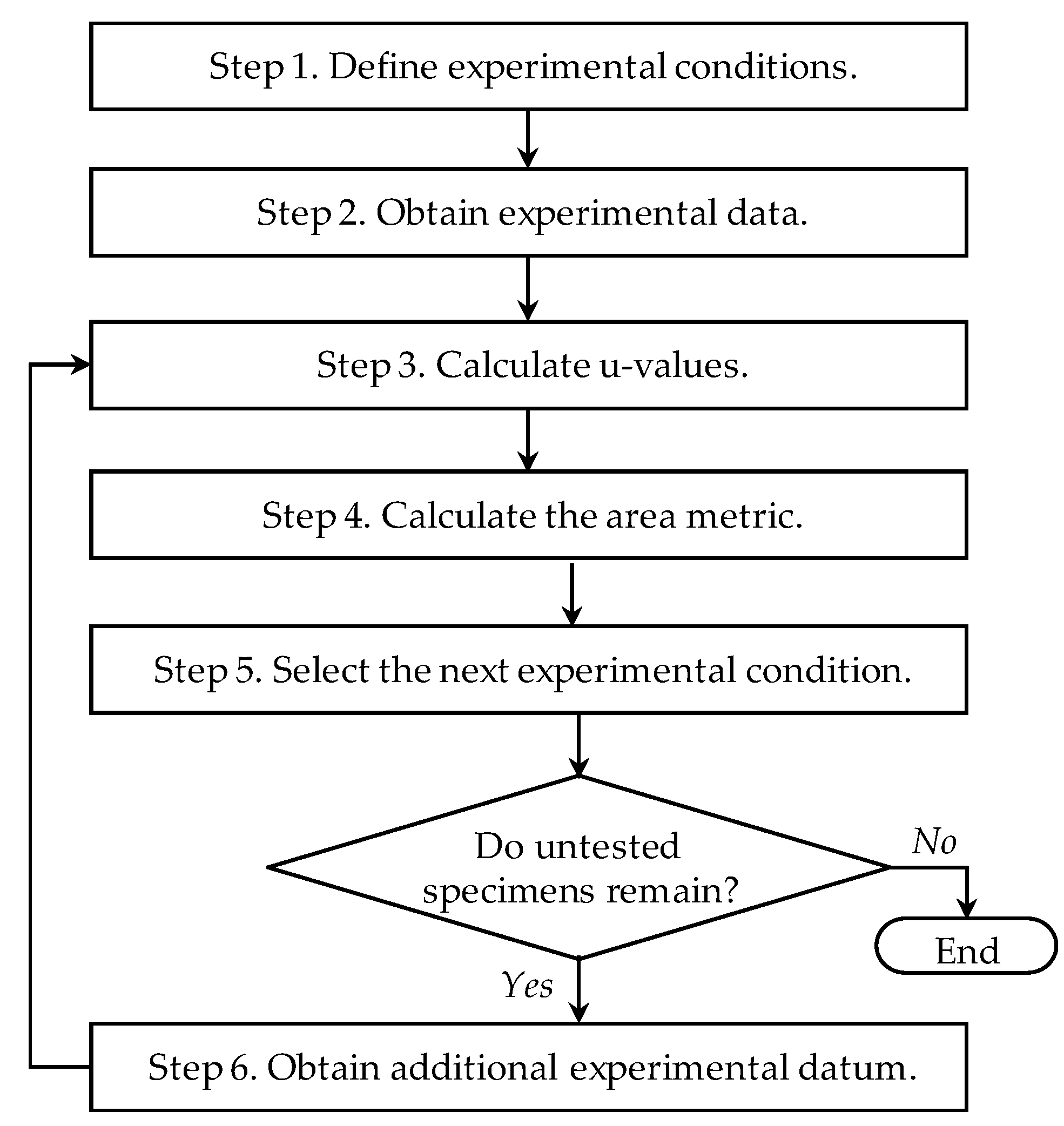
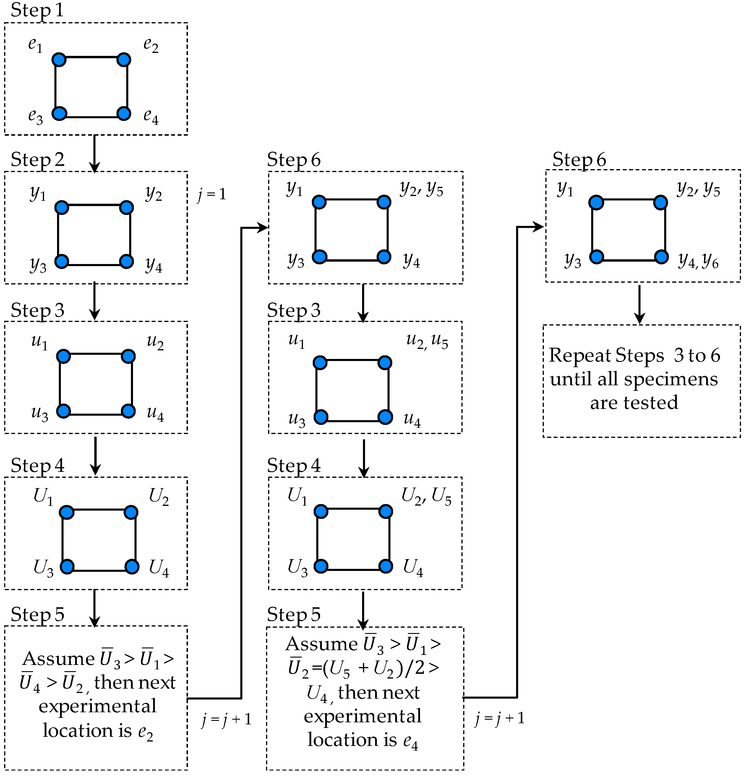
3.1. Procedure of Experimental Design

The relationship between the observed response (y) and the predicted response (ψ) of a computational model can be defined.
y ( ζ ) + e = ψ ( ζ , β ) + δ , ζ Ω s , β Ω l
where ζ is the vector of operation variables {ζ1, ζ2, …, ζs} (e.g., operational conditions and environmental temperature); β is the vector of model variables {β1, β2, …, βl}; s and l are the number of the operation and model variables, respectively; and e and δ are the measurement and modeling errors, respectively. In HTVC, e and δ are considered to be encompassed in y and ψ, unless the true functions of e and δ are quantified explicitly [18]. The effect of bad and missing data on classification problems was discussed in [13].
For the model validation, additional experimental data in a validation domain are required. Experimental conditions are typically designed with model variables and operation variables in a validation domain. Thus, the vector of design variables (θ) can be defined.
θ = { β 1 , β 2 , , β v , ζ 1 , ζ 2 , , ζ w } , θ Ω ( v + w ) , v l , w s
The procedure for RAED consists of six steps as shown in Figure 3.
Step 1: Determine design variables and levels for factorial design. The level of individual design variables can be determined based on characteristics of the predicted model (e.g., linearity, nonlinearity, statistical variance), characteristics of design variables (e.g., continuous variable, discrete variable, boundary of the variables), the number of available test specimens, and expert opinions. Then, define experimental conditions based on the selected factorial design (e.g., full factorial and fractional factorial). The total number of experimental conditions (N) is calculated based on the number of design variables, levels of design variables, and the selected factorial design. The vector of experimental conditions can be defined as e = {e1, e2, …, eN}. Individual experimental conditions are the combination of various environmental and operational conditions.
Step 2: Obtain a single experimental datum (yi) at individual experimental conditions. i expresses the order of the test data. j is set to be one. Then, N number of experimental data is obtained. The sets of an experimental datum for given experimental conditions are {y1 | e1}, {y2 | e2}, …, {yN | eN}.
Step 3: Calculate u-values by using Equation (1) for experimental data. A list of a set that combines the u-value with the experimental datum for the given test condition is {u1, y1| e1}, {u2, y2| e2}, …, {uN, yN| eN}.
Step 4: Calculate the area metrics (U) of each set in Step 3 using all u-values except ui. For example, U1 is calculated using {u2, u3, …, uN} and UN is calculated using {u1, u2, …, uN−1}. The sets of the area metric, u-value, experimental datum and test condition are {U1, u1, y1| e1}, {U2, u2, y2| e2}, …, {UN, uN, yN| eN}.
Step 5: Make groups of U values that have an identical experimental condition and calculate the mean of the U values for each group. The sets of means of U values and test conditions are { U ¯ 1 | e1}, { U ¯ 2 | e2}, …, { U ¯ N | eN}. Find the set having the smallest U value mean and define the (N + j)th experimental condition, es(N+j), as the same experimental condition of the selected set. The subscript s indicates the number of the experimental condition, which is between 1 and N. If untested specimens remain, go to Step 6. Otherwise, terminate.
Step 6: Obtain (N + j)th experimental datum at the experimental condition, es(N+j). The sets of an experimental datum for each given experimental condition are {y1 | e1}, {y2 | e2}, …, {yi | eN}, {yN+1 | es(N+j)}. Set j = j + 1. Go to Step 3.
To present the procedures step by step, an example is shown in Figure 4. In this example, a two-level factorial design with two design variables is shown. However, any variation of the design can be made.

3.2. Experimental Design for Reduction of Type II Error

As explained in Section 3.1, RAED selects the next experimental setting as the condition where the calculated area metric (U) is smaller than other conditions. The lower area metric indicates that the predicted PDF is not closer to the mother distribution of the experimental data. In this section, with deductive reasoning, the relation between the low area metric and the reduction of type II error is studied. The type II errors of two hypothetical experimental conditions are compared. It is worth noting that any variation of the experimental conditions can be made. The use of a particular set of experimental conditions does not limit the applicability of the proposed RAED method to extended problems.
Experimental condition I: The mother distribution of the experimental results (i.e., performance of interest (PoI)) is a standard normal distribution (f0 ~ Normal (0, 1)) and the PDF of the predicted results is a normal distribution (e.g., f1 ~ Normal (0.56, 1)), as shown in Figure 5. A predefined number of experimental data (e.g., eighteen) are randomly obtained from the f0 to calculate the area metric. The number of experimental data is determined by considering the additional experimental resources available.
Experimental condition II: The mother distribution of the experimental results is also a standard normal distribution (f0). However, the PDF of the predicted results is a normal distribution (e.g., f2 ~ Normal (1.05, 1)), as shown in Figure 5. A predefined number of experimental data (e.g., eighteen) are randomly obtained from the f0 to calculate the area metric.
It is certain that the predicted model, f2, is more invalid and has a lower area metric than the predicted model, f1, when they are compared with the mother distribution of the experimental results, f0. The type II error of each experimental condition can be calculated using the PDF of the area metric (fu,n(x)) and the following equation. The null hypothesis is the claim that the computational model is valid, while the alternative hypothesis is the claim that the computational model is not valid.
Type   II   error = 0 D n ( α ) f u , n ( x ) d x
For the quantification, it is assumed that type I error is 0.1 (the significant level in Equation (3)). Figure 6 shows the PDF of the area metric of experimental conditions I and II. The procedure for constructing the PDFs of the area metric is described as follows.
Step 1: Determine a virtual sampling size (k) and the experimental data size (n). Here, k and n are 5000 and 18, respectively.
Step 2: Generate samples (x1, x2, …, xn) randomly from the mother distribution of the experimental data.
Step 3: Calculate the CDF values (u1, u2, …, un) corresponding to yi using Equation (1).
Step 4: Calculate the area metric (U) using Equation (2).
Step 5: Repeat Steps 2 to 4, k times to generate random data (U1, U2, …, Uk). Then construct the empirical PDF of area metric (fu,n(x)) using U values. In this paper, the Pearson system [19] is used to construct empirical PDFs of the U values.
Table 2 shows the calculated type II error of experimental conditions I and II. The type II error of experimental condition II is lower than that of experimental condition I. The calculated results show that type II error can be minimized if more test data are sampled at the experimental condition where the difference between the PDF of predicted results and the mother distribution of the experimental data is larger than other conditions.
The difficulty in designing experiments for model validation is that we do not have any idea about the mother distribution of the experimental data. Thus, RAED employs an adaptive process to determine the next experimental condition based on pre-obtained experimental results.

4. Case Study

In real engineering applications, it is almost impossible to know the mother distribution of the experimental data since this would require an infinite number of experimental samples. To overcome the challenge, simulation samples generated by numerical models are often used. For instance, the use of numerical models is considered as a natural way in the study of phenomena arising in applied sciences [20,21] such as the diffusion and transport of pollutants in the atmosphere [22], the dissipation of nonlinear waves [23,24], and the growth models in ecology and oncology. In this case study, a numerical model is employed to quantify type II error and to show the effectiveness of the proposed RAED method. The numerical model (ψ) is devised to have a generic exponential form with one random variable (β), one operating variable (ζ), and two model parameters (p and q).
ψ = (p × β) × ζq
The exponential form well represents various engineering applications, such as friction of a rubber material [25], fatigue of a solder joint [26], and transient thermal conduction [27]. For example, the friction model (μ) of a rubber material [25] is a function of contact pressure (φ) with two model parameters: (1) friction coefficient μ0 at a reference contact pressure φref and (2) pressure exponential parameter υ0. Two model parameters can be figured out with experimental data obtained at different operating conditions of contact pressure.
μ = μ 0 × ( φ φ r e f ) ν 0
To demonstrate the proposed RAED method, we assumed that the predicted model and the mother function of the experimental results have different parameter values.
Predicted model:
ψ = (p × β) × ζq; p = 1.0, q = 1.0
Mother function of experimental results∶
y = (p × β) × ζq; p = 0.896, q = 1.1
where β is the random variable that follows a normal distribution with the mean of 1.0 and the standard deviation of 0.5; ζ is the operating variable that is assumed to be between three and seven (i.e., 3 ≤ ζ ≤ 7). The confidence intervals of the mother function of the experiments (y) and the predicted model (ψ) are in the validation domain, as depicted in Figure 7. The predicted model represents the experimental results when ζ is set to three. In contrast, the difference between y and ψ stays larger as ζ is increased to seven. With an assumption of having eighteen samples for model validation, three different experimental designs were considered to show the benefits of RAED, including:
Experimental Design A: Consider three levels of different operating conditions (ζ = 3, 5 and 7) and obtain six data points at each level.
Experimental Design B: Obtain eighteen data points at operating conditions evenly distributed between 3 ≤ ζ ≤ 7.
Experimental Design C: Consider three levels of different operating conditions (ζ = 3, 5 and 7) and obtain eighteen data points using RAED.
The PDFs of the area metric (U) were constructed according to the three designs by following the steps outlined in Section 3.1. It was assumed that the virtual sampling size (k) was 10,000 and the number of sampled data (i.e., the number of test specimens) was eighteen. The PDFs of individual area metrics are shown in Figure 8. Experimental data were sampled based on the three designs A, B and C. It was confirmed that the fu,18 of Design C shifted further to the right than the distributions of Designs A and B. Table 3 summarizes the statistical information and type II error of the PDFs. It was confirmed that type II error of Design C was lower than the error of the other designs. A histogram in Figure 9 shows the number of data obtained at each operating condition in the case of Design C. A single experimental datum was first obtained at each operating condition as explained in Step 2 in Section 3.1. For example, one datum was obtained at individual operating conditions, ζ = 3, 5 and 7. Next, the remaining data of 15 were obtained one by one at operating conditions determined by Steps 3, 4, and 5. Since at least two data were obtained at identical operating conditions, the maximum number of sampled data at individual operating conditions was 16 as shown in Figure 9. It was confirmed that more samples were obtained at the condition where the operating condition (ζ) was seven. At that condition, the difference between the predicted and experimental results was larger than that observed for other operating conditions (ζ was three and five).

5. Conclusions

This paper presented a new method to design validation experiments called response-adaptive experiment design (RAED) for computational models in mechanics. The RAED method adaptively selects the next experimental condition from among candidates of various operating conditions (experimental settings). RAED consists of six key steps: (1) define experimental conditions, (2) obtain experimental data, (3) calculate u-values, (4) compute the area metric, (5) select the next experimental condition, and (6) obtain additional experimental datum. To demonstrate the effectiveness of the RAED method, a case study of a numerical example was shown. The case study accounted for real engineering applications in the field. It was shown that RAED can effectively reduce type II error (the possibility of accepting an invalid computational model) during model validation. RAED can also help to avoid unnecessary experiments for model validation by allocating validation resources effectively.
The existing study based on HTVC only considered type I error (or significance level) to evaluate whether a computational model is valid. The HTVC-based approach does not provide any way to reduce type II error. Different from the HTVC-based approach, this study proposed a response-adaptive experiment design (RAED) approach for model validation with limited experimental samples. The RAED-based approach can reduce type II error while maintaining type I error at an acceptable level, especially for the validation of computational models of safety-related and mission-critical systems.
Future works are suggested in two folds. First, the adequacy of the proposed method will be evaluated after implementing to a real system. This paper employed a numerical example to demonstrate the effectiveness of the proposed method. Second, further improvement of RAED will be made to account for the effect of a modeling errors on RAED. Experimental data can be collected at the condition where the prediction capability of computational models is dependent on modeling errors. The modeling errors are another source for failing model validation, which was ignored in this study.

Author Contributions

Conceptualization, B.C.J.; formal analysis, Y.-H.S.; funding acquisition, B.C.J. and H.O.; investigation, S.H.L.; methodology, B.C.J.; project administration, B.C.J.; resources, Y.C.H.; writing—original draft, B.C.J.; writing—review and editing, H.O. All authors have read and agreed to the published version of the manuscript.

Funding

This research was supported by the Korea Institute of Energy Technology Evaluation and Planning (KETEP) and the Ministry of Trade, Industry & Energy (MOTIE) of the Republic of Korea (No.20171520000250, No.20162010104420), and partially supported by the main project of Korea Institute of Machinery and Materials (Project Code: NK213E).

Conflicts of Interest

The authors declare no conflict of interest.

References

  1. Park, J.; Ha, J.M.; Oh, H.; Youn, B.D.; Choi, J.; Kim, N.H. Model-based fault diagnosis of a planetary gear: A novel approach using transmission error. IEEE Trans. Reliab. 2016, 65, 1830–1841. [Google Scholar] [CrossRef]
  2. Oh, H.; Choi, H.; Jung, J.H.; Youn, B.D. A robust and convex metric for unconstrained optimization in statistical model calibration—Probability residual (PR). Struct. Multidiscip. Optim. 2019, 60, 1171–1187. [Google Scholar] [CrossRef]
  3. IEEE. IEEE Standard for Software Verfication and Validation; Institute of Electrical and Electronic Engineers: New York, NY, USA, 1998; pp. 1–80. [Google Scholar]
  4. ASME. Guide for Verification and Validation in Computational Solid Mechanics; American Society of Mechanical Engineers: New York, NY, USA, 2006; pp. 1–36. [Google Scholar]
  5. Oberkampf, W.L.; Trucano, T.G.; Hirsch, C. Verification, validation, predictive capability in computational engineering and physics. Appl. Mech. Rev. 2004, 57, 345–384. [Google Scholar] [CrossRef] [Green Version]
  6. Thacker, B.H.; Doebling, S.W.; Hemez, F.M.; Anderson, M.C.; Pepin, J.E.; Rodriguez, E.A. Concepts of Model Verification and Validation; Los Alamos National Laboratory: Los Alamos, NM, USA, 2004; pp. 1–27. [Google Scholar]
  7. Oberkampf, W.L.; Barone, M.F. Measures of agreement between computation and experiment: Validation metrics. J. Comput. Phys. 2006, 217, 5–36. [Google Scholar] [CrossRef] [Green Version]
  8. Youn, B.D.; Jung, B.C.; Xi, Z.; Kim, S.B.; Lee, W.R. A hierarchical framework for statistical model calibration in engineering product development. Comput. Methods Appl. Mech. Eng. 2011, 200, 1421–1431. [Google Scholar] [CrossRef]
  9. Zhang, R.X.; Mahadevan, S. Bayesian methodology for reliability model acceptance. Reliab. Eng. Syst. Saf. 2003, 80, 95–103. [Google Scholar] [CrossRef]
  10. Chen, W.; Tsui, K.; Wang, S. A design-driven validation approach using Bayesian prediction models. J. Mech. Des. 2008, 140, 021101. [Google Scholar] [CrossRef]
  11. Liu, F.; Bayarri, M.J.; Berger, J.O.; Paulo, R.; Sacks, J. A Bayesian analysis of the thermal challenge problem. Comput. Methods Appl. Mech. Eng. 2008, 197, 2457–2466. [Google Scholar] [CrossRef]
  12. Jung, B.C.; Park, J.; Oh, H.; Kim, J.; Youn, B.D. A framework of model validation and virtual product qualification with limited experimental data based on statistical inference. Struct. Multidiscip. Optim. 2015, 51, 573–583. [Google Scholar] [CrossRef]
  13. Mohammadi, F.; Zheng, C. A precise SVM classification model for predictions with missing data. In Proceedings of the 4th National Conference on Applied Research in Electrical, Mechanical Computer and IT Engineering, Tehran, Iran, 4 October 2018; pp. 3594–3606. [Google Scholar]
  14. Angus, J.E. The probability integral transform and related results. SIAM Rev. 1994, 36, 652–654. [Google Scholar] [CrossRef]
  15. Ferson, S.; Oberkampf, W.L.; Ginzburg, L. Model validation and predictive capability for the thermal challenge problem. Comput. Methods Appl. Mech. Eng. 2008, 197, 2408–2430. [Google Scholar] [CrossRef]
  16. Tavoosi, J.; Mohammadi, F. Design a New Intelligent Control for a Class of Nonlinear Systems. In Proceedings of the 6th International Conference on Control, Instrumentation, and Automation (ICCIA 2019), Kordestan, Iran, 30–31 October 2019. [Google Scholar]
  17. Karimi, H.; Ghasemi, R.; Mohammadi, F. Adaptive Neural Observer-Based Nonsingular Terminal Sliding Mode Controller Design for a Class of Nonlinear Systems. In Proceedings of the 6th International Conference on Control, Instrumentation, and Automation (ICCIA 2019), Kordestan, Iran, 30–31 October 2019. [Google Scholar]
  18. Oh, H.; Kim, J.; Son, H.; Youn, B.D.; Jung, B.C. A systematic approach for model refinement considering blind and recognized uncertainties in engineered product development. Struct. Multidiscip. Optim. 2016, 54, 1527–1541. [Google Scholar] [CrossRef]
  19. Youn, B.D.; Xi, Z.; Wang, P. Eigenvector dimension reduction (EDR) method for sensitivity-free probability analysis. Struct. Multidiscip. Optim. 2008, 37, 13–28. [Google Scholar] [CrossRef]
  20. Rebenda, J.; Smarda, Z.; Khan, Y. A new semi-analytical approach for numerical solving of Cauchy problem for differential equations with delay. Filomat 2017, 31, 4725–4733. [Google Scholar] [CrossRef]
  21. Fazio, R.; Jannelli, A.; Agreste, S. A finite difference method on non-uniform meshes for time-fractional advection—Diffusion equations with a source term. Appl. Sci. 2018, 8, 960. [Google Scholar] [CrossRef] [Green Version]
  22. Ruggieri, M.; Speciale, M.P. Similarity reduction and closed form solutions for a model derived from two-layer fluids. Adv. Differ. Equ. 2013, 2013, 355. [Google Scholar] [CrossRef] [Green Version]
  23. Ruggieri, M. Kink solutions for a class of generalized dissipative equations. Abstr. Appl. Anal. 2012, 2012, 7. [Google Scholar] [CrossRef]
  24. Ruggieri, M.; Valenti, A. Approximate symmetries in nonlinear viscoelastic media. Bound. Value Probl. 2013, 2013, 143. [Google Scholar] [CrossRef] [Green Version]
  25. Cho, J.C.; Jung, B.C. Prediction of tread pattern wear by an explicit finite element model. Tire Sci. Technol. 2007, 35, 276–299. [Google Scholar] [CrossRef]
  26. Oh, H.; Wei, H.P.; Han, B.; Youn, B.D. Probabilistic lifetime prediction of electronic packages using advanced uncertainty propagation analysis and model calibration. IEEE Trans. Compon. Packag. Manuf. Technol. 2016, 6, 238–248. [Google Scholar] [CrossRef]
  27. Dowding, K.J.; Pilch, M.; Hills, R.G. Formulation of the thermal problem. Comput. Methods Appl. Mech. Eng. 2008, 197, 2385–2389. [Google Scholar] [CrossRef]
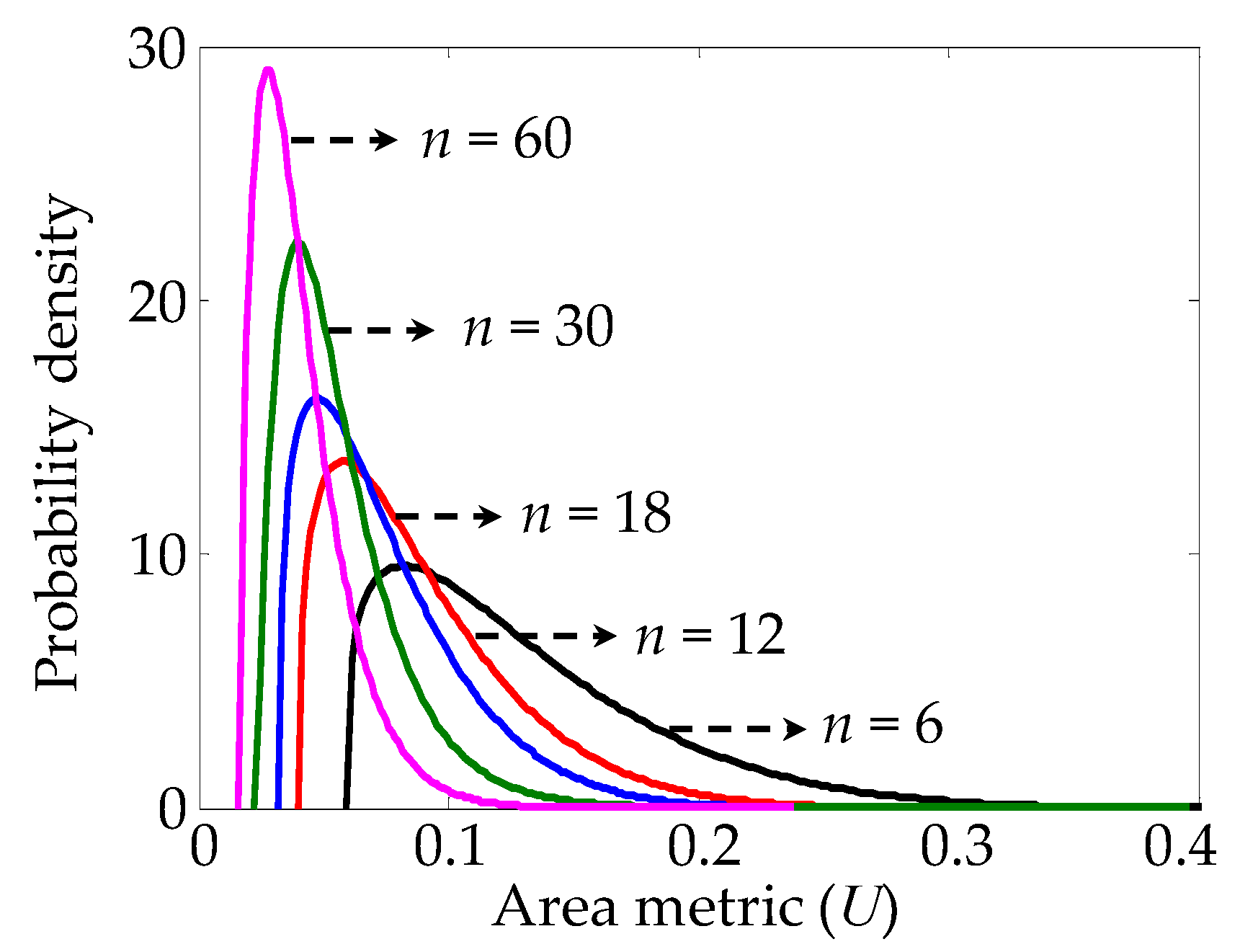
Figure 1. Validation activities for computational models in mechanics [8].
Applsci 10 00647 g001
Figure 2. Probability density functions (PDFs) of the area metric according to experimental data sizes.
Applsci 10 00647 g002
Figure 3. Flow diagram of the proposed response-adaptive experiment design method.
Applsci 10 00647 g003
Figure 4. Example of RAED: Two-level factorial design with two design variables.
Applsci 10 00647 g004
Figure 5. PDFs of the experimental and predicted results.
Applsci 10 00647 g005
Figure 6. PDFs of the area metric (U) for experimental conditions I and II.
Applsci 10 00647 g006
Figure 7. Confidence intervals and means of y and Ψ.
Applsci 10 00647 g007
Figure 8. PDF of each area metric (U) for the three design conditions.
Applsci 10 00647 g008
Figure 9. Histogram of the number of sampled data at each operating condition. (a) ζ = 3; (b) ζ = 5; (c) ζ = 7.
Applsci 10 00647 g009
Table 1. Statistical moments of the PDFs of the area metric (all rows follow a Pearson’s type I distribution).
nMeanStandard DeviationSkewnessKurtosis
60.12960.05351.13264.2585
120.09140.03891.23374.7938
180.07410.03191.21774.6966
300.05690.02471.48716.3728
600.04070.01781.32455.3782
Table 2. Calculated type II errors.
CasesType II Error
Condition I0.35
Condition II0.00
Table 3. Statistical information of the fu,18 for the three experimental designs.
Experimental DesignMeanStandard DeviationSkewnessKurtosisPearson System TypeType II Error
Design A0.21900.0542−0.05662.8346Type I0.068
Design B0.23900.0562−0.17612.8332Type I0.040
Design C0.32060.0675−1.06434.6404Type I0.016

