A Comparative Study of Different Machine Learning Algorithms in Predicting the Content of Ilmenite in Titanium Placer

Abstract

In this study, the ilmenite content in beach placer sand was estimated using seven soft computing techniques, namely random forest (RF), artificial neural network (ANN), k-nearest neighbors (kNN), cubist, support vector machine (SVM), stochastic gradient boosting (SGB), and classification and regression tree (CART). The 405 beach placer borehole samples were collected from Southern Suoi Nhum deposit, Binh Thuan province, Vietnam, to test the feasibility of these soft computing techniques in estimating ilmenite content. Heavy mineral analysis indicated that valuable minerals in the placer sand are zircon, ilmenite, leucoxene, rutile, anatase, and monazite. In this study, five materials, namely rutile, anatase, leucoxene, zircon, and monazite, were used as the input variables to estimate ilmenite content based on the above mentioned soft computing models. Of the whole dataset, 325 samples were used to build the regarded soft computing models; 80 remaining samples were used for the models’ verification. Root-mean-squared error (RMSE), determination coefficient (R²), a simple ranking method, and residuals analysis technique were used as the statistical criteria for assessing the model performances. The numerical experiments revealed that soft computing techniques are capable of estimating the content of ilmenite with high accuracy. The residuals analysis also indicated that the SGB model was the most suitable for determining the ilmenite content in the context of this research.

1. Introduction

In the context of the intense development of the world, the demand for machinery, paint, paper, and plastic is virtually unending with titanium minerals labelled as one of the primary materials [1,2,3]. This commodity can be exploited from the placer and hard rocks deposits [4]. In particular, placer deposits are abundant sources of titanium for coastal countries and Vietnam is one of those countries [5]. They are considered to be economically valuable minerals because of their ease of exploitation and flexibility [6]. In titanium placer, the major mineral components are ilmenite, rutile, anatase, leucoxene, zircon, and monazite [7]. Of those minerals, ilmenite and rutile are normally considered as the main types containing titanium because of their high proportion in the total heavy minerals [8,9]. Although the concentration of TiO₂ is higher in natural rutile than ilmenite, the distribution of rutile is normally inadequate for processing in titanium placer. Furthermore, sulfate and chloride processes can be applied as the chemical methods to obtain higher TiO₂ content [10,11]. In other words, TiO₂ can be enriched from ilmenite by chemical methods [12,13,14,15]. Therefore, ilmenite can be considered as the main mineral used to extract TiO₂ in titanium placer.

In recent years, mineral exploration based on data-driven or artificial intelligence (AI) techniques is considered as a cost-effective alternative to traditional methods. The spatial and geochemical datasets have been analyzed by traditional analytical or AI approaches with high reliability [16,17,18,19,20]. Mineralization, as well as minerals, can be forecasted using these techniques to highlight mineral potential based on similar data attributes [21]. For example, the ant colony algorithm was performed to recognize the geochemical anomalies in the interpolated concentration of Au, Cu, Ag, Zn, and Pb by Chen, An [22]. The artificial neural network (ANN), k-nearest neighbors (kNN) models were also developed to investigate the components of mineral of coal and maceral groups by Mlynarczuk, Skiba [23]. To evaluate the relationship between mineral potentials as well as establish mineral prospectivity maps, Maepa, Smith [24] used ANN, fuzzy logic, and logistics regression as powerful tools for the mapping of potential gold deposits. Zuo, Xiong [25] also deployed several machine learning (ML) techniques to identify geochemical anomalies of Fe polymetallic deposits. They concluded that ML techniques are robust tools for discovering multivariate geochemistry anomalies. In another study, Johnson et al. [18] used ANN with 96 data points to evaluate the distribution of geochemical of gold deposits at Canning Basin (Western Australia). Their results showed that ANN was a feasible technique for assessing geochemical property distribution with a determination coefficient (R²) of 0.8. To establish another approach to geochemical mapping, Zuo et al. [26] applied deep learning and indicated that this method could deal with nonlinear and complex problems. In addition, various ML techniques have been used to detect the content as well as the potential of minerals and geochemical anomalies as the following works [18,25,27,28,29,30,31,32,33,34].

Review of the published works shows that the mapping of mineral distribution can be achieved by using data-driven techniques. Although a number of studies have been carried out to model several commodities, such as Fe, Au, Zn, Cu, there is still a scarcity of research on titanium in general and ilmenite in particular. Motivated from the significance of this type of mineral on the local economy [35], this study aimed at evaluating the feasibility of predicting it using different AI techniques. From extensive review of previous works, seven different AI methods presenting four groups were selected: Decision tree algorithms group (random forest (RF) and classification and regression tree (CART), boosting algorithms group (stochastic gradient boosting (SGB)), neural networks group (ANN), and nonlinear algorithms groups (support vector machine (SVM), cubist, and kNN). Based on the obtained results, the best method will be introduced as the state-of-the-art technique for predicting ilmenite content.

2. Background of Artificial Intelligence Techniques Used

2.1. Random Forest

As described by Breiman [36] first, RF is a decision tree algorithm in statistical communication. It is known as a useful tool for classification and regression issues. Inspired from an election, each decision tree acts as a voter. The set of all votes for the final decision is used to improve the predictions’ accuracy [37,38,39]. The background of the RF algorithm can be described according to the following pseudo-code (Figure 1).

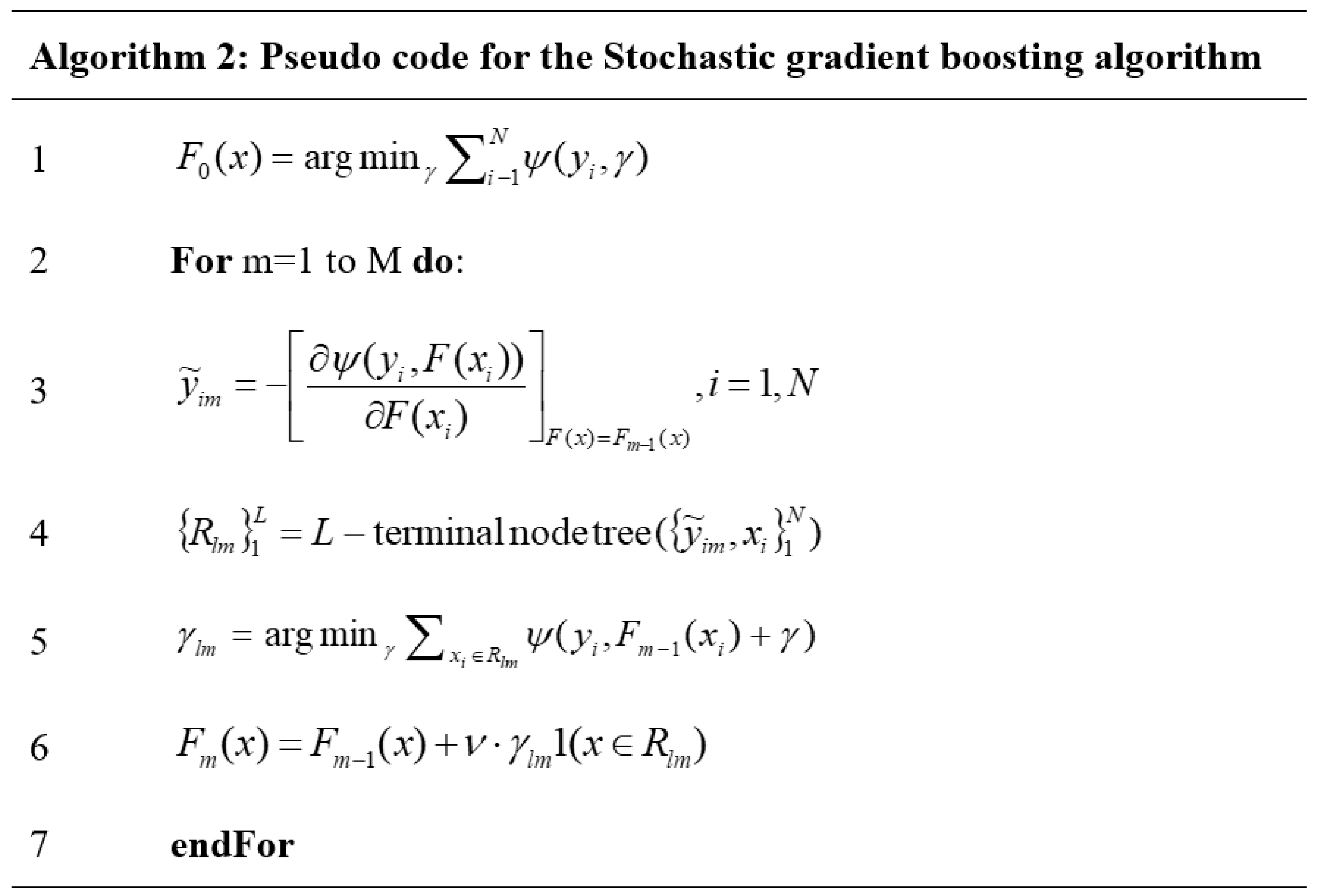
2.2. Stochastic Gradient Boosting

SGB is one of the ensemble techniques proposed by Friedman [41]. Based on decision tree algorithm [42,43], SGB was improved by using boosting learning and editing error of decision trees. Like RF technique, SGB can solve all classification, as well as regression issues. The theory of SGB algorithm is shown in Figure 2.

2.3. CART

In data mining, CART was introduced as an effective nonparametric algorithm for forecasting issues, including regression and classification. Additionally, it is also known as a robust decision tree algorithm for forecasting problems [44]. Inspired by the development of trees in nature, CART’s operational principles are developed based on mapping data [45]. Variables in data are represented by internal nodes (i.e., rutile, anatase, leucoxene, zircon, and monazite). The leaf nodes represent the outcomes (i.e., ilmenite content).

Unlike other techniques, CART does not require data normalization and can work well with outliers [46]. Furthermore, the CART algorithm can clearly explain situations as a “white box algorithm” [47]. Additionally, statistical tests can be applied to model verification to increase their reliability. More details of the CART algorithm can be found in [48,49,50,51].

2.4. SVM

SVM is well known as a benchmark AI technique in the statistical community. It can be applied for forecasting/predicting any regression/classification issues [52]. The SVM theory is based on the minimization of structural risk [53,54].

For regression problems, the functions of the kernel are often to be used to predict resulting outcome, such as radial basis function (RBF), two neural networks, polynomial, sigmoid and linear, exponential radial basis function (ERBF) [55,56]. In recent years, SVM has been applied in many fields as well as publications, therefore, the details of the SVM are not presented in this study but can be found in [57,58,59,60,61,62,63].

2.5. Cubist

As well-developed rule-based model, Cubist algorithm (CA) was proposed by Quinlan [64] and widely introduced by Rulequest [65]. It works on the idea of the nearest neighbors in the set of training data with additional corrections [66]. Like the M5′ Rules model, the CA can generate the rules for forecasting classification and regression issues [67]. On the other hand, CA is classified as a decision tree technique. Although it also creates an initial tree as the first step, however, unlike the M5 tree model, the rule is generated by the pruning the tree (collapses the paths). For regression issues (e.g., prediction of ilmenite content), the dataset is defined by the rules, and the CA model can fit for each rule. To avoid overfitting in CA, the rules can be combined or pruned. Subsequently, split-caused pruned are smoothed to compensate for the sharp discontinuities. Briefly, the CA can be described in four steps, as illustrated in Figure 3.

2.6. The k-Nearest Neighbors

In machine learning, kNN is classified as a lazy algorithm [68,69]. It stores all observations that it reads then predicts other observations based on distance functions. The goal of kNN is to compute a numerical target averaged from the k nearest neighbors [70]. In addition, the inverse distance weighted average is also used for computing such distance [71]. For regression problems, kNN uses three distance functions to compute the distance between the neighbors as follow:

$$\mathrm{Euclidean}\mathrm{function}:\sqrt{{\displaystyle \sum _{i=1}^f{(x_i-y_i)}^2}}$$

(1)

$$\mathrm{Manhattan}\mathrm{function}:{\displaystyle \sum _{i=1}^f\left|x_i-y_i\right|}$$

(2)

$$\mathrm{Minkowski}\mathrm{function}:{\left({\displaystyle \sum _{i=1}^f{\left(\left|x_i-y_i\right|\right)}^q}\right)}^{1/q}$$

(3)

where x_i and y_i are the ith-dimensions of the x and y points; q is the order between two points x and y.

2.7. ANN

As a model of information processing, ANN was introduced and simulated based on the idea of the human brain [72]. It is capable of processing information quickly and accurately based on the connections of neurons. In fact, ANN is also considered to be smarter than humans as they are capable of energetic calculations and self-evolution [73]. ANN can learn problems quickly and remember them. Then, based on the experience acquired, it can predict new observations [74].

There are many types of ANN, such as multilayer perceptron neural network (MLP), recurrent neural network (RNN), and convolutional neural network (CNN) to name a few. However, MLP is still a popular technique due to its simplicity and efficiency [75,76]. Therefore, this study used an MLP-type ANN model. Accordingly, its structure consists of three parts: Input layer (i.e., rutile, anatase, leucoxene, zircon, and monazite), hidden layers, and output layer (i.e., ilmenite content).

The operation method of ANN for estimating the ilmenite content is as follows:

• Step 1: The input neurons receive signals from the external environment (the weight percent of each heavy mineral: Rutile, anatase, leucoxene, zircon, and monazite).
• Step 2: Calculate weights and biases.
• Step 3: Send information that has been preprocessed to the first hidden layer. Transfer functions can be enabled to transmit information between layers.
• Step 4: Perform learning and calculation in the first hidden layer.
• Step 5: Recalculate weights and biases after learning in the first hidden layer.
• Step 6: Send the results to the second hidden layer,
• Step 7: Perform the same actions as done in the first hidden layer.
• Step 8: Send the calculation results, weights, and biases in the second hidden layer to the output layer.
• Step 9: Repeat the same calculations for the next hidden layer.
• Step 10: Estimate the ilmenite content and produce the final result.

3. Data Collection

The study area is the Southern Suoi Nhum titanium placer deposit, Binh Thuan province (Vietnam), as shown in Figure 4. The previous geological surveys indicated that the study area and surroundings have loess sediments of the Pleistocene to Holocene age. These Quaternary sediments are distributed into sandy strips running parallel to the coastline. Exploration results showed that the mineral components of the placer sand consist mainly of ilmenite, rutile, anatase, leucoxene, zircon, and monazite (Figure 5). Among these heavy minerals, ilmenite is a common mineral and accounts for a significant proportion. These minerals exist in the red marine sediment of the Pleistocene age (Phan Thiet formation) and a gray marine-eolian residue of the Holocene age. Deo Ca Complex can be found in the surrounding areas. The complex consist of whitish-gray grano-syenite, biotite granite, and biotite-hornblende granite [35].

For data collection, placer sand samples were dried and mixed thoroughly in the laboratory. The samples were then sieved using the 1.18 mm (American Society for Testing and Materials) ASTM sieve. The coning and quartering method was applied continuously to reduce the sample to 20–30 g. The ultrafine clays in the samples were removed using distilled water. After drying, the total heavy minerals (THM) were isolated by using bromoform heavy liquid. The magnetic/nonmagnetic heavy materials in THM were separated using hand magnets. Then, each type of heavy mineral (ilmenite, rutile, anatase, leucoxene, zircon, and monazite) was determined by manual grain counting using an optical microscope. Finally, the weight percentage of individual heavy minerals was calculated by multiplying their percentage with the respective specific gravity values. In this study, 405 samples were collected from different positions of the mine. Scanning electron microscope ((SEM) Quanta 450, FEI company) with energy-dispersive X-ray spectroscopy (EDS) was used to double-check the identified heavy minerals through their morphology and composition. In order to prepare the samples for SEM-EDS analysis, the heavy minerals were put onto the surface of carbon conductive tape that attached to the specimen stub. The samples were then coated by carbon to enhance the quality of SEM images.

In this study area, ilmenite is a common mineral and accounts for a significant proportion. For AI calculation, the weight percent of each heavy mineral (i.e., rutile, anatase, leucoxene, zircon, and monazite) were used as input data for predicting ilmenite content (not titanium content in each heavy mineral). The statistical properties of the heavy minerals are listed in

Table 1. Statistical attributes of the weight percent of each heavy mineral.

Classification	Rutile	Anatase	Leucoxene	Zircon	Monazite	Ilmenite
Min.:	0.000	0.000	0.000	0.013	0.001	0.188
1st Qu.:	0.001	0.0001	0.003	0.030	0.001	0.306
Median:	0.001	0.0001	0.005	0.052	0.001	0.424
Mean:	0.001343	0.0001573	0.008	0.064	0.003	0.467
3rd Qu.:	0.002	0.0002	0.012	0.080	0.002	0.538
Max.:	0.009	0.0007	0.032	0.306	0.058	2.246

.

In

Table 2. Correlation matrix of heavy minerals.

	Rutile	Anatase	Leucoxene	Zircon	Monazite	Ilmenite
Rutile	1
Anatase	0.659115	1
Leucoxene	0.516591	0.447161	1
Zircon	0.65455	0.632258	0.326362	1
Monazite	0.101687	0.037384	0.084057	0.052774	1
Ilmenite	0.476926	0.650812	0.04358	0.668171	−0.00484	1

, the correlation matrix of input and output variables is presented. In the cases of high positive/negative correlations (above approximately 0.75 or below −0.75), they may adversely affect the performance of the models [77]. As a positive sign, all the pairs of attributes in Table 2 are insignificant. Therefore, they have been designated as independent variables to estimate the dependent variable. The feasibility of the AI techniques was assessed by explaining the complicated relationship between predictors and response variable.

4. Development of the Model

In order to develop the ilmenite content prediction models, the dataset was separated into two groups according to previous studies [60,78,79]. Specifically, 80% of the original dataset (325 samples) was used to train the models, called the training dataset; 20% remaining of the data (80 samples) was used to validate the model, called the testing dataset. Note that the same sets of training and testing data were used during developing and evaluating of all models. For development of the mentioned model, R software (version 4.5) was used based on their packages.

4.1. RF Model

For the RF modeling, the number of trees in the forest (ntree) and the randomly selected predictors (mtry) were used to adjust the accuracy of the model. The k-fold cross-validation method was applied with k = 10 to avoid overfitting of the model. According to Nguyen, Bui [80], ntree should be selected as 2000 to ensure the forest richness. Subsequently, mtry was set from 1 to 50 for finding out the best RF’s parameters. Ultimately, the optimal RF model was detected with mtry = 2 and ntree = 2000, as shown in Figure 6.

4.2. SGB Model

For the SGB model, the boosting iterations ($\alpha$), max tree depth ($\beta$), shrinkage ($\chi$), and minimum terminal node size ($\delta$) were specifically fine-tuned for developing the SGB model. Like the RF model, a 10-fold cross-validation method was also applied to avoid over/underfitting. A trial and error procedure with various parameters of 100 SGB models was performed. The best modelling result was achieved by using $\alpha$ = 141, $\beta$ = 4, $\chi$ = 0.1899, and $\delta$ = 5. Figure 7 shows the root-mean-squared error (RMSE) of the SGB model for estimating the content of ilmenite in this study with different parameters.

4.3. CART Model

Herein, the optimal CART model was considered and built using only one parameter, which is complexity parameter (cp) and a grid search technique with cp lies from 0 to 0.1 with interval of 0.002. Numerical experiments showed that cp = 0.002 was the best for the CART model in estimating ilmenite content. Figure 8 shows the structure of the CART model for forecasting ilmenite content in this work.

4.4. SVM Model

For SVM modelling, various kernel functions can be applied, such as linear, nonlinear, radial basis function (RBF), polynomial, and sigmoid, where RBF is the most-often used one for regression problems [56,61,81,82]. Thus, RBF kernel function was applied for SVM in this study, and $\sigma$ and C (cost) were the significant parameters being fine-turned. There were 100 SVM models using different values of these two parameters performed, and the best result was achieved with $\sigma$ = 0.009 and C = 83.219, as shown in Figure 9.

4.5. Cubist Model

With the cubist model, the rules worked based on the committee ($\epsilon$) and neighbors/instances ($\varphi$). A “trial and error” procedure of $\epsilon$ and $\varphi$ was utilized to find out the best cubist model, as shown in Figure 10. Herein, a grid search technique was applied for $\epsilon$ and $\varphi$ (i.e., $\varphi$ = 0 to 9, $\epsilon$ = 4 to 99). Eventually, the optimal cubist model was determined with $\epsilon$ = 37 and $\varphi$ = 2.

4.6. The kNN Model

For modeling the ilmenite content by the kNN model, the maximum of the neighbors ($\phi$), the distance between neighbors ($\gamma$), and kernel function were used to establish the kNN model in this study. Eight kernel functions were applied for the kNN model in this study, including biweight, cosin, epanechnikov, Gaussian, inverse, rectangular, triangular, and triweight. A series of kNN models were tried with various values of $\phi$ and $\gamma$ to find out the best kNN model. As a result, $\phi$ = 71 and $\gamma$ = 0.215 with the inverse kernel function were the best for the kNN model. Figure 11 shows the performance of the kNN model for estimating the content of ilmenite in this study.

4.7. ANN Model

For ANN modelling, the hidden layers and neurons per layer need to be chosen carefully. Too many hidden layers or neurons can lead to overfitting [83]. In addition, they can affect the processing time of the model. Therefore, ANNs with two or three hidden layers were recommended by Nguyen et al. [61] for the simple regression problems. In this study, an ANN model with a structure with two hidden layers was selected to estimate the ilmenite content. Its structure includes 5, 16, 10, and 1 neurons, for the input, the first and second hidden, and output layers, respectively (Figure 12). Unlike the previous models, the min-max scale method was applied to normalize the dataset in the range of (−1 to 1); 50 repetitions were performed to determine the initial weights and biases of the ANN model. Subsequently, the optimal weights and biases of the ANN model were calculated, as shown in Figure 12 through the black and grey lines.

5. Performance Indicators for Evaluating the Soft Computing Techniques

In the present study, root-mean-squared error (RMSE), coefficient of correlation (R²), ranking method, and residuals analysis technique were used to rate the models’ quality. The performance indicators are computed as follow:

$$\mathrm{RMSE}=\sqrt{\frac{1}{n}{\displaystyle \sum _{i=1}^n{(y_{i.ilmenite}-{\widehat{y}}_{i.ilmenite})}^2}}$$

(4)

$${\mathrm{R}}^2=1-\frac{{\displaystyle \sum _i(y_{i.ilmenite}-{\widehat{y}}_{i.ilmenite}}{)}^2}{{\displaystyle \sum _i{(y_{i.ilmenite}-\overline{y})}^2}}$$

(5)

where n is a total number of experimental datasets; $y_{i.ilmenite}$_, ${\widehat{y}}_{i.ilmenite}$ and $\overline{y}$ are measured, predicted, and mean of $y_i$ values, respectively.

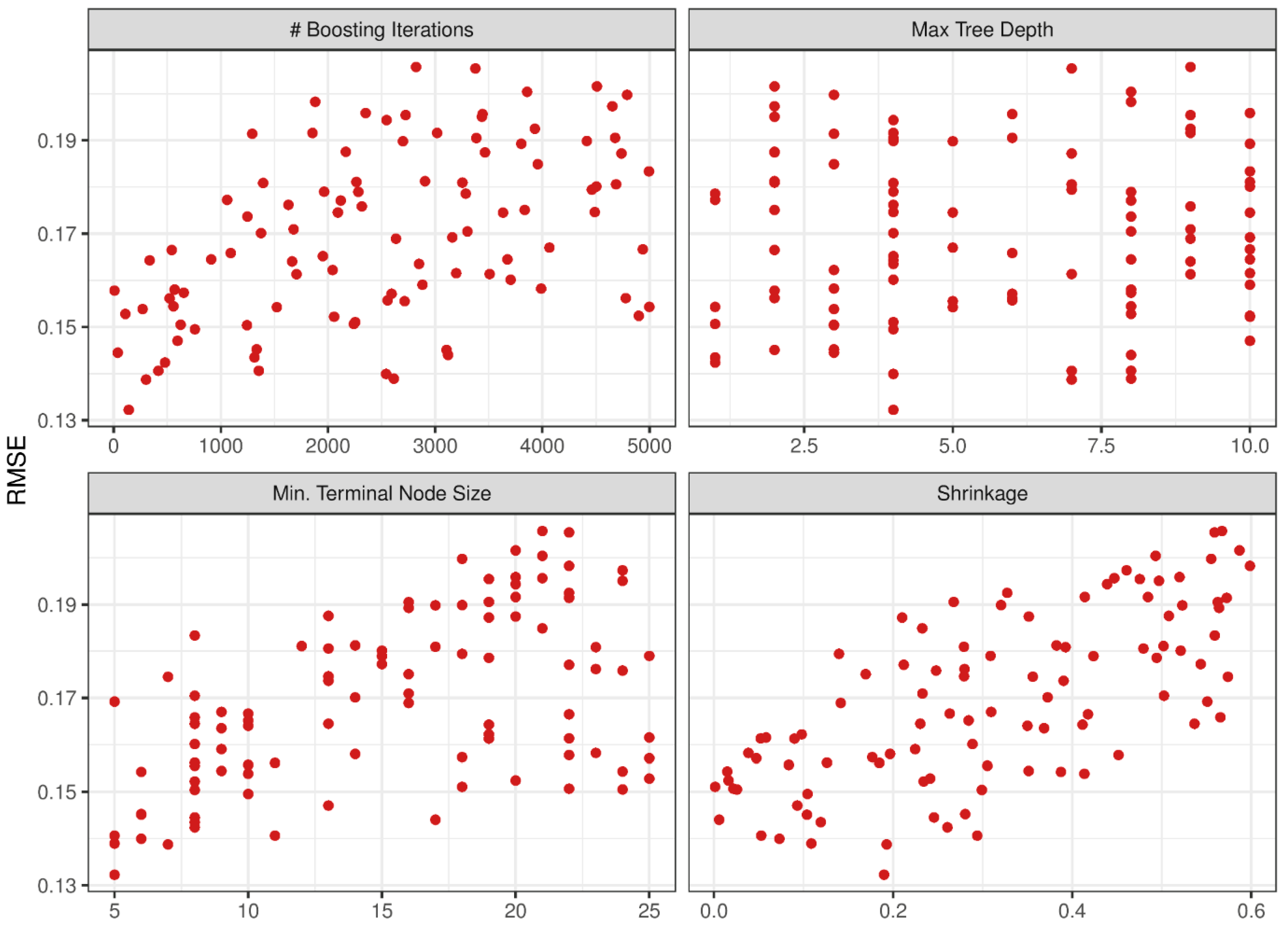
6. Results and Discussions

After developing the models, their performance was compared and evaluated using RMSE and R², ranking, and residual plots being analyzed. Based on the training dataset, the ilmenite content predictive models (i.e., SVM, RF, SGB, CART, kNN, cubist, and ANN) were developed as described above.

Table 3. Performance of the soft computing techniques for estimating ilmenite content (training dataset).

Model	RMSE	R2	Rank for RMSE	Rank for R2	Total Ranking Score	Sort
SVM	0.134	0.692	2	2	4	6
CART	0.147	0.675	1	1	2	7
kNN	0.122	0.747	6	6	12	2
RF	0.127	0.737	5	5	10	3
SGB	0.132	0.716	3	3	6	5
Cubist	0.128	0.720	4	4	8	4
ANN	0.091	0.860	7	7	14	1

calculates the indicators of performance of the soft computing techniques for estimating the content of ilmenite in the training process.

Performance of the developed soft computing models in Table 3 showed that all the AI models were able to generate reasonably accurate ilmenite content estimation. Most models provided good performance with R² over 0.7 where some achieved R² over 0.8. Additionally, based on the ranking index, the ANN is the best model on the training dataset. To verify the performances of the stated soft computing techniques, 80 experimental datasets on the set of testing data was used as described above. Model validation is considered as the most critical step in the model building sequence.

Table 4. Performance of the soft computing techniques for estimating ilmenite content (testing dataset).

Model	RMSE	R2	Rank for RMSE	Rank for R2	Total Ranking Score	Sort
SVM	0.092	0.780	1	3	4	5
CART	0.082	0.817	4	4	8	4
kNN	0.092	0.766	1	1	2	7
RF	0.080	0.824	6	6	12	2
SGB	0.081	0.818	5	5	10	3
Cubist	0.078	0.830	7	7	14	1
ANN	0.092	0.774	1	2	3	6

computes the performance on the models using the testing dataset based on performance indicators.

From Table 4, there are some differences from Table 3. Whereas the ANN is the best soft computing model on the training dataset, the cubist model with the highest performances, as well as the ranking, became the best model on the testing dataset. At the other end, the kNN model with the lowest performances and ranking on validation set also became the worst model on the testing dataset. Notably, although the ANN model on the training data set was the top scorer, its performance decreased significantly on the test set. It showed the unstable nature of ANN model in estimating the ilmenite content in this study. The RF and SGB models still retained the same stable performance as on the training dataset. Figure 13 shows the accuracy of the developed models on the testing dataset through R² values.

Although the R² values of the models were high, they did not guarantee that the models fit the data well. Therefore, the residuals analysis of the models was conducted in order to check the assumptions of independence, normality, and homoscedasticity. The histogram (Figure 14) and the normal probability plots (Figure 15) were used to check whether or not it is justifiable to suppose that the random errors inherent in the developed soft computing models were extracted from a normal distribution.

Based on histogram plots of the residuals of the models (Figure 14), we can see that most of the residuals of the models are Gaussian or normal distribution. It suggested that the models fit the data well. Notably, the residuals of the SGB and cubist models seem to be better fitted to the normal distribution. Additionally, the frequency of the SGB model appears to be more stable than the cubist model. The residuals of the SGB model are smaller and approximate random errors. These points showed that the SGB model seems to be the most suitable model for the data used in this study.

Furthermore, the quantile-quantile plots (Q-Q plots) were used (Figure 15) in order to confirm the normality of the data for the developed models. Figure 15 shows the normality of the residuals of the models visually. If the SGB model and cubist model were good candidates for the data of this study in Figure 14, then, in Figure 15, the SGB model shows that it was more suitable for the data than the cubist model. Based on the results of Table 3 and Table 4 and the residual analysis of the models (Figure 14 and Figure 15), the SGB model should be selected as the best soft computing technique for estimating the ilmenite content in this study.

7. Conclusions

Ilmenite is a fairly common and industrially valuable titanium-containing mineral in coastal placer mines, including in Vietnam. In this study, 405 samples from the Suoi Nhum mine, Vietnam, were collected and processed to separate different heavy minerals. The weight percents of each heavy mineral (rutile, anatase, leucoxene, zircon, and monazite) were used as input data for predicting ilmenite content by AI techniques. The obtained results of this work indicated that ilmenite content and the remaining other heavy minerals are highly correlated.

As a conclusion, AI is a robust technique that can be applied in practical engineering to determine the content of ilmenite in titanium placer/beach placer sand with a significant reliability. This study demonstrated that the SGB model is the best model for estimating ilmenite content. Additionally, the cubist model can also be used in practical engineering. The remaining models (kNN, RF, SVM, CART, and ANN) were also considered in other conditions or areas. It helps to investigate and define potential heavy mineral areas more appropriately. On the other hand, the results of this research are the basis for selecting the mineral mining areas in the placer mines more reasonably.

References

1. Lasheen, T. Chemical benefication of Rosetta ilmenite by direct reduction leaching. Hydrometallurgy 2005, 76, 123–129. [Google Scholar] [CrossRef]
2. Nayl, A.; Awwad, N.; Aly, H. Kinetics of acid leaching of ilmenite decomposed by KOH: Part 2. Leaching by H2SO4 and C2H2O4. J. Hazard. Mater. 2009, 168, 793–799. [Google Scholar] [CrossRef] [PubMed]
3. Nayl, A.; Ismail, I.; Aly, H. Ammonium hydroxide decomposition of ilmenite slag. Hydrometallurgy 2009, 1, 196–200. [Google Scholar] [CrossRef]
4. Mehdilo, A.; Irannajad, M.; Rezai, B. Applied mineralogical characterization of ilmenite from Kahnuj placer deposit, Southern Iran. Period. Mineral. 2015, 84, 289–302. [Google Scholar]
5. Kušnír, I. Mineral resources of Vietnam. Acta Montan. Slovaca 2000, 2, 165–172. [Google Scholar]
6. Dung, N.T.; Bac, B.H.; Van Anh, T.T. Distribution and Reserve Potential of Titanium-Zirconium Heavy Minerals in Quang an Area, Thua Thien Hue Province, Vietnam. In Proceedings of the International Conference on Geo-Spatial Technologies and Earth Resources, Hanoi, Vietnam, 5–6 October 2017; pp. 326–339. [Google Scholar]
7. Lalomov, A.; Platonov, M.; Tugarova, M.; Bochneva, A.; Chefranova, A. Rare metal–titanium placer metal potential of Cambrian–Ordovician sandstones in the northwestern Russian Plate. Lithol. Miner. Resour. 2015, 50, 501–511. [Google Scholar] [CrossRef]
8. Force, E.R. Geology of Titanium-Mineral Deposits; Geological Society of America: McLean, Vietnam, 1991; Volume 259. [Google Scholar]
9. Dill, H.; Melcher, F.; Fuessl, M.; Weber, B. The origin of rutile-ilmenite aggregates (“nigrine”) in alluvial-fluvial placers of the Hagendorf pegmatite province, NE Bavaria, Germany. Mineral. Petrol. 2007, 89, 133–158. [Google Scholar] [CrossRef]
10. Gázquez, M.J.; Bolívar, J.P.; Garcia-Tenorio, R.; Vaca, F. A review of the production cycle of titanium dioxide pigment. Mater. Sci. Appl. 2014, 5, 441. [Google Scholar] [CrossRef] [Green Version]
11. Mwase Malumbo, J.; Gaydardzhiev, S.; Guillet, A.; Stefansecu, E.; Sehner, E. Investigation on Ilmenite Placer Ore as a Precursor for Synthetic Rutile. In Proceedings of the EMPRC 2018 European Mineral Processing and Recycling Congress, Clausthal-Zellerfeld, Germany, 25–26 June 2018. [Google Scholar]
12. Korneliussen, A.; McENROE, S.A.; Nilsson, L.P.; Schiellerup, H.; Gautneb, H.; Meyer, G.B.; Storseth, L. An overview of titanium deposits in Norway. Nor. Geol. Unders. 2000, 436, 27–38. [Google Scholar]
13. Samal, S.; Mohapatra, B.; Mukherjee, P.; Chatterjee, S. Integrated XRD, EPMA and XRF study of ilmenite and titania slag used in pigment production. J. Alloys Compd. 2009, 474, 484–489. [Google Scholar] [CrossRef]
14. Zhang, S.; Liu, S.; Ma, W.; Dai, Y. Review of TiO2-Rich Materials Preparation for the Chlorination Process. In TMS Annual Meeting & Exhibition; Springer: Berlin/Heidelberg, Germany, 2018; pp. 225–234. [Google Scholar]
15. Perks, C.; Mudd, G. Titanium, zirconium resources and production: A state of the art literature review. Ore Geol. Rev. 2019, 107, 629–646. [Google Scholar] [CrossRef]
16. Achieng, K.O. Modelling of soil moisture retention curve using machine learning techniques: Artificial and deep neural networks vs support vector regression models. Comput. Geosci. 2019, 133, 104320. [Google Scholar] [CrossRef]
17. Conway, D.; Alexander, B.; King, M.; Heinson, G.; Kee, Y. Inverting magnetotelluric responses in a three-dimensional earth using fast forward approximations based on artificial neural networks. Comput. Geosci. 2019, 127, 44–52. [Google Scholar] [CrossRef]
18. Johnson, L.M.; Rezaee, R.; Kadkhodaie, A.; Smith, G.; Yu, H. Geochemical property modelling of a potential shale reservoir in the Canning Basin (Western Australia), using Artificial Neural Networks and geostatistical tools. Comput. Geosci. 2018, 120, 73–81. [Google Scholar] [CrossRef]
19. Souza, J.; Santos, M.; Magalhães, R.; Neto, E.; Oliveira, G.; Roque, W. Automatic classification of hydrocarbon “leads” in seismic images through artificial and convolutional neural networks. Comput. Geosci. 2019, 132, 23–32. [Google Scholar] [CrossRef]
20. Trépanier, S.; Mathieu, L.; Daigneault, R.; Faure, S. Precursors predicted by artificial neural networks for mass balance calculations: Quantifying hydrothermal alteration in volcanic rocks. Comput. Geosci. 2016, 89, 32–43. [Google Scholar] [CrossRef] [Green Version]
21. Juliani, C.; Ellefmo, S.L. Prospectivity Mapping of Mineral Deposits in Northern Norway Using Radial Basis Function Neural Networks. Minerals 2019, 9, 131. [Google Scholar] [CrossRef] [Green Version]
22. Chen, Y.; An, A. Application of ant colony algorithm to geochemical anomaly detection. J. Geochem. Explor. 2016, 164, 75–85. [Google Scholar] [CrossRef]
23. Mlynarczuk, M.; Skiba, M. The application of artificial intelligence for the identification of the maceral groups and mineral components of coal. Comput. Geosci. 2017, 103, 133–141. [Google Scholar] [CrossRef]
24. Maepa, F.; Smith, R. Predictive mapping of the gold mineral potential in the Swayze Greentone Belt, ON, Canada. In SEG Technical Program Expanded Abstracts 2017; Society of Exploration Geophysicists: Tulsa, OK, USA, 2017; pp. 2456–2460. [Google Scholar]
25. Zuo, R.; Xiong, Y. Big data analytics of identifying geochemical anomalies supported by machine learning methods. Nat. Resour. Res. 2018, 27, 5–13. [Google Scholar] [CrossRef]
26. Zuo, R.; Xiong, Y.; Wang, J.; Carranza, E.J.M. Deep learning and its application in geochemical mapping. Earth Sci. Rev. 2019, 192, 1–14. [Google Scholar] [CrossRef]
27. Chen, Y.; Lu, L.; Li, X. Application of continuous restricted Boltzmann machine to identify multivariate geochemical anomaly. J. Geochem. Explor. 2014, 140, 56–63. [Google Scholar] [CrossRef]
28. Ekbia, H.; Mattioli, M.; Kouper, I.; Arave, G.; Ghazinejad, A.; Bowman, T.; Suri, V.R.; Tsou, A.; Weingart, S.; Sugimoto, C.R. Big data, bigger dilemmas: A critical review. J. Assoc. Inf. Sci. Technol. 2015, 66, 1523–1545. [Google Scholar] [CrossRef] [Green Version]
29. Gonbadi, A.M.; Tabatabaei, S.H.; Carranza, E.J.M. Supervised geochemical anomaly detection by pattern recognition. J. Geochem. Explor. 2015, 157, 81–91. [Google Scholar] [CrossRef]
30. Liu, Y.; Ma, S.; Zhu, L.; Sadeghi, M.; Doherty, A.L.; Cao, D.; Le, C. The multi-attribute anomaly structure model: An exploration tool for the Zhaojikou epithermal Pb-Zn deposit, China. J. Geochem. Explor. 2016, 169, 50–59. [Google Scholar] [CrossRef]
31. Nykänen, V.; Niiranen, T.; Molnár, F.; Lahti, I.; Korhonen, K.; Cook, N.; Skyttä, P. Optimizing a knowledge-driven prospectivity model for gold deposits within Peräpohja Belt, Northern Finland. Nat. Resour. Res. 2017, 26, 571–584. [Google Scholar] [CrossRef]
32. Parsa, M.; Maghsoudi, A.; Yousefi, M. A receiver operating characteristics-based geochemical data fusion technique for targeting undiscovered mineral deposits. Nat. Resour. Res. 2018, 27, 15–28. [Google Scholar] [CrossRef]
33. Hronsky, J.M.; Kreuzer, O.P. Applying Spatial Prospectivity Mapping to Exploration Targeting: Fundamental Practical issues and Suggested Solutions for the Future. Ore Geol. Rev. 2019, 107, 647–653. [Google Scholar] [CrossRef]
34. Wang, Z.; Zuo, R.; Dong, Y. Mapping Geochemical Anomalies Through Integrating Random Forest and Metric Learning Methods. Nat. Resour. Res. 2019, 28, 1285–1298. [Google Scholar] [CrossRef]
35. Khang, L.Q. Report on Exploration of Titan-Zircon Heavy Minerals at South Suoi Nhum, Ham Thuan Nam District, Binh Thuan Province; Center for Information and Archives of Geology: Hanoi, Vietnam, 2011.
36. Breiman, L. Random forests. Mach. Learn. 2001, 45, 5–32. [Google Scholar] [CrossRef] [Green Version]
37. Vigneau, E.; Courcoux, P.; Symoneaux, R.; Guérin, L.; Villière, A. Random forests: A machine learning methodology to highlight the volatile organic compounds involved in olfactory perception. Food Qual. Prefer. 2018, 68, 135–145. [Google Scholar] [CrossRef]
38. Matin, S.; Farahzadi, L.; Makaremi, S.; Chelgani, S.C.; Sattari, G. Variable selection and prediction of uniaxial compressive strength and modulus of elasticity by random forest. Appl. Soft Comput. 2018, 70, 980–987. [Google Scholar] [CrossRef]
39. Cánovas-García, F.; Alonso-Sarría, F.; Gomariz-Castillo, F.; Oñate-Valdivieso, F. Modification of the random forest algorithm to avoid statistical dependence problems when classifying remote sensing imagery. Comput. Geosci. 2017, 103, 1–11. [Google Scholar] [CrossRef] [Green Version]
40. Anderson, G.; Pfahringer, B. Random Relational Rules. Ph.D. Thesis, Department of Computer Science, University of Waikato, Hamilton, New Zealand, 2009. [Google Scholar]
41. Friedman, J.H. Stochastic gradient boosting. Comput. Stat. Data Anal. 2002, 38, 367–378. [Google Scholar] [CrossRef]
42. Friedman, J.H. Greedy function approximation: A gradient boosting machine. Ann. Stat. 2001, 29, 1189–1232. [Google Scholar] [CrossRef]
43. Czajkowski, M.; Kretowski, M. The role of decision tree representation in regression problems–An evolutionary perspective. Appl. Soft Comput. 2016, 48, 458–475. [Google Scholar] [CrossRef]
44. Hamze-Ziabari, S.; Bakhshpoori, T. Improving the prediction of ground motion parameters based on an efficient bagging ensemble model of M5′ and CART algorithms. Appl. Soft Comput. 2018, 68, 147–161. [Google Scholar] [CrossRef]
45. Choubin, B.; Moradi, E.; Golshan, M.; Adamowski, J.; Sajedi-Hosseini, F.; Mosavi, A. An Ensemble prediction of flood susceptibility using multivariate discriminant analysis, classification and regression trees, and support vector machines. Sci. Total Environ. 2019, 651, 2087–2096. [Google Scholar] [CrossRef]
46. Kantardzic, M. Data Mining: Concepts, Models, Methods, and Algorithms; John Wiley & Sons: Hoboken, NJ, USA, 2011. [Google Scholar]
47. Larose, D.T.; Larose, C.D. Discovering Knowledge in Data: An Introduction to Data Mining; John Wiley & Sons: Hoboken, NJ, USA, 2014. [Google Scholar]
48. De’ath, G.; Fabricius, K.E. Classification and regression trees: A powerful yet simple technique for ecological data analysis. Ecology 2000, 81, 3178–3192. [Google Scholar] [CrossRef]
49. Steinberg, D.; Colla, P. CART: Classification and regression trees. In The Top Ten Algorithms in Data Mining; Chapman and Hall/CRC: New York, NY, USA, 2009; pp. 193–216. [Google Scholar]
50. Timofeev, R. Classification and Regression Trees (CART) Theory and Applications; Humboldt University: Berlin, Germany, 2004. [Google Scholar]
51. Breiman, L. Classification and Regression Trees, 1st ed.; Routledge: New York, NY, USA, 2017. [Google Scholar] [CrossRef]
52. Wang, G.; Carr, T.R.; Ju, Y.; Li, C. Identifying organic-rich Marcellus Shale lithofacies by support vector machine classifier in the Appalachian basin. Comput. Geosci. 2014, 64, 52–60. [Google Scholar] [CrossRef]
53. Cortes, C.; Vapnik, V. Support vector machine. Mach. Learn. 1995, 20, 273–297. [Google Scholar] [CrossRef]
54. Dohare, A.K.; Kumar, V.; Kumar, R. Detection of myocardial infarction in 12 lead ECG using support vector machine. Appl. Soft Comput. 2018, 64, 138–147. [Google Scholar] [CrossRef]
55. Zendehboudi, A.; Baseer, M.; Saidur, R. Application of support vector machine models for forecasting solar and wind energy resources: A review. J. Clean. Prod. 2018, 199, 272–285. [Google Scholar] [CrossRef]
56. Nguyen, H. Support vector regression approach with different kernel functions for predicting blast-induced ground vibration: A case study in an open-pit coal mine of Vietnam. SN Appl. Sci. 2019, 1, 283. [Google Scholar] [CrossRef] [Green Version]
57. Zhou, J.; Li, X.; Shi, X. Long-term prediction model of rockburst in underground openings using heuristic algorithms and support vector machines. Saf. Sci. 2012, 50, 629–644. [Google Scholar] [CrossRef]
58. Hemmati-Sarapardeh, A.; Shokrollahi, A.; Tatar, A.; Gharagheizi, F.; Mohammadi, A.H.; Naseri, A. Reservoir oil viscosity determination using a rigorous approach. Fuel 2014, 116, 39–48. [Google Scholar] [CrossRef]
59. Tian, Y.; Fu, M.; Wu, F. Steel plates fault diagnosis on the basis of support vector machines. Neurocomputing 2015, 151, 296–303. [Google Scholar] [CrossRef]
60. Bui, X.N.; Nguyen, H.; Le, H.A.; Bui, H.B.; Do, N.H. Prediction of Blast-induced Air Over-pressure in Open-Pit Mine: Assessment of Different Artificial Intelligence Techniques. Nat. Resour. Res. 2019. [Google Scholar] [CrossRef]
61. Nguyen, H.; Drebenstedt, C.; Bui, X.-N.; Bui, D.T. Prediction of Blast-Induced Ground Vibration in an Open-Pit Mine by a Novel Hybrid Model Based on Clustering and Artificial Neural Network. Nat. Resour. Res. 2019. [Google Scholar] [CrossRef]
62. Gonzalez-Abril, L.; Angulo, C.; Nuñez, H.; Leal, Y. Handling binary classification problems with a priority class by using Support Vector Machines. Appl. Soft Comput. 2017, 61, 661–669. [Google Scholar] [CrossRef]
63. De Almeida, B.J.; Neves, R.F.; Horta, N. Combining Support Vector Machine with Genetic Algorithms to optimize investments in Forex markets with high leverage. Appl. Soft Comput. 2018, 64, 596–613. [Google Scholar] [CrossRef]
64. Quinlan, J.R. Learning with continuous classes. In Proceedings of the 5th Australian Joint Conference on Artificial Intelligence, Hobart, Australia, 16–18 November 1992; pp. 343–348. [Google Scholar]
65. Rulequest. Data Mining with Cubist. RuleQuest Research Pty Ltd., St. Ives, NSW, Australia. Available online: https://wwwrulequestcom/cubist-infohtml (accessed on 15 November 2019).
66. Wang, Y.; Witten, I.H. Induction of model trees for predicting continuous classes. Presented at the Ninth European Conference on Machine Learning, Prague, Czech Republic, 23–25 April 1997. [Google Scholar]
67. Butina, D.; Gola, J.M. Modeling aqueous solubility. J. Chem. Inf. Comput. Sci. 2003, 43, 837–841. [Google Scholar] [CrossRef]
68. Altman, N.S. An introduction to kernel and nearest-neighbor nonparametric regression. Am. Stat. 1992, 46, 175–185. [Google Scholar]
69. Rezaei, Z.; Selamat, A.; Taki, A.; Rahim, M.S.M.; Kadir, M.R.A. Automatic plaque segmentation based on hybrid fuzzy clustering and k nearest neighborhood using virtual histology intravascular ultrasound images. Appl. Soft Comput. 2017, 53, 380–395. [Google Scholar] [CrossRef]
70. Silva-Ramírez, E.-L.; Pino-Mejías, R.; López-Coello, M. Single imputation with multilayer perceptron and multiple imputation combining multilayer perceptron and k-nearest neighbours for monotone patterns. Appl. Soft Comput. 2015, 29, 65–74. [Google Scholar] [CrossRef]
71. Pu, Y.; Zhao, X.; Chi, G.; Zhao, S.; Wang, J.; Jin, Z.; Yin, J. Design and implementation of a parallel geographically weighted k-nearest neighbor classifier. Comput. Geosci. 2019, 127, 111–122. [Google Scholar] [CrossRef]
72. Tkáč, M.; Verner, R. Artificial neural networks in business: Two decades of research. Appl. Soft Comput. 2016, 38, 788–804. [Google Scholar] [CrossRef]
73. Crowder, J.A.; Carbone, J.; Friess, S. Artificial Creativity and Self-Evolution: Abductive Reasoning in Artificial Life Forms. In Artificial Psychology: Psychological Modeling and Testing of AI Systems; Springer International Publishing: Cham, Switzerland, 2020; pp. 65–74. [Google Scholar] [CrossRef]
74. Karayiannis, N.; Venetsanopoulos, A.N. Artificial Neural Networks: Learning Algorithms, Performance Evaluation, and Applications; Springer Science & Business Media: New York, NY, USA, 2013; Volume 209. [Google Scholar]
75. Mocanu, D.C.; Mocanu, E.; Stone, P.; Nguyen, P.H.; Gibescu, M.; Liotta, A. Scalable training of artificial neural networks with adaptive sparse connectivity inspired by network science. Nat. Commun. 2018, 9, 2383. [Google Scholar] [CrossRef] [Green Version]
76. Mishra, A.; Chandra, P.; Ghose, U.; Sodhi, S.S. Bi-modal derivative adaptive activation function sigmoidal feedforward artificial neural networks. Appl. Soft Comput. 2017, 61, 983–994. [Google Scholar] [CrossRef]
77. Chatfield, C. Introduction to Multivariate Analysis, 1st ed.; Routledge: New York, NY, USA, 1980. [Google Scholar] [CrossRef]
78. Moayedi, H.; Armaghani, D.J. Optimizing an ANN model with ICA for estimating bearing capacity of driven pile in cohesionless soil. Eng. Comput. 2018, 34, 347–356. [Google Scholar] [CrossRef]
79. Nguyen, H.; Bui, X.-N.; Tran, Q.-H.; Mai, N.-L. A new soft computing model for estimating and controlling blast-produced ground vibration based on hierarchical K-means clustering and cubist algorithms. Appl. Soft Comput. 2019, 77, 376–386. [Google Scholar] [CrossRef]
80. Nguyen, H.; Bui, X.-N. Predicting Blast-Induced Air Overpressure: A Robust Artificial Intelligence System Based on Artificial Neural Networks and Random Forest. Nat. Resour. Res. 2019, 28, 893–907. [Google Scholar] [CrossRef]
81. Olatomiwa, L.; Mekhilef, S.; Shamshirband, S.; Mohammadi, K.; Petković, D.; Sudheer, C. A support vector machine–firefly algorithm-based model for global solar radiation prediction. Sol. Energy 2015, 115, 632–644. [Google Scholar] [CrossRef]
82. Qian, X.; Yang, M.; Wang, C.; Li, H.; Wang, J. Leaf magnetic properties as a method for predicting heavy metal concentrations in PM2.5 using support vector machine: A case study in Nanjing, China. Environ. Pollut. 2018, 242, 922–930. [Google Scholar]
83. Nguyen, H.; Bui, X.-N.; Bui, H.-B.; Mai, N.-L. A comparative study of artificial neural networks in predicting blast-induced air-blast overpressure at Deo Nai open-pit coal mine, Vietnam. Neural Comput. Appl. 2018, 1–17. [Google Scholar] [CrossRef]
Figure 1. Random forest’s (RF) pseudo-code [40].
Applsci 10 00635 g001
Figure 2. Pseudo-code of the stochastic gradient boosting (SGB) technique. Reproduced with permission from [41], Copyright Elsevier, 2002.
Applsci 10 00635 g002
Figure 3. Cubist model and its operation for estimating ilmenite component.
Applsci 10 00635 g003
Figure 4. A view of the Southern Suoi Nhum titanium placer mine (Vietnam).
Applsci 10 00635 g004
Figure 5. Images of the placer sand in the study area. (A) Placer sand, (B) placer ore, (C,D) SEM images of placer ore, (E) EDS results of minerals.
Applsci 10 00635 g005
Figure 6. Performance of RF model for estimating ilmenite content.
Applsci 10 00635 g006
Figure 7. Performance of the SGB model in this study.
Applsci 10 00635 g007
Figure 8. The structure of the classification and regression tree (CART) model for estimating ilmenite content.
Applsci 10 00635 g008
Figure 9. Performance of the support vector machine (SVM) model in this study.
Applsci 10 00635 g009
Figure 10. Performance of the cubist model in predicting ilmenite content.
Applsci 10 00635 g010
Figure 11. Performance of the k-nearest neighbors (kNN) model in this study.
Applsci 10 00635 g011
Figure 12. Artificial neural network (ANN) model for estimating the content of ilmenite.
Applsci 10 00635 g012
Figure 13. Predicted/measured parameters of the soft computing techniques used herein.
Applsci 10 00635 g013
Figure 14. Histogram plots of the residuals of the models.
Applsci 10 00635 g014
Figure 15. Normal probability plots of the residuals of the soft computing techniques herein.
Applsci 10 00635 g015